跳到论文正文
W Papers独立论文阅读器 arXiv:1102.3642 论文正文 计算阅读时间 · 0%
引用这篇论文根据当前论文元数据生成,正式投稿前建议核对。


License: arXiv.org perpetual non-exclusive license
arXiv:1102.3642v1 [math.CA] 17 Feb 2011

Tangent-point repulsive potentials
for a class of non-smooth mm-dimensional sets in ℝn{\mathbb{R}}^{n}.
Part I: Smoothing and self-avoidance effects

Paweł Strzelecki    Heiko von der Mosel
version of August 24, 2026
Abstract

We consider repulsive potential energies ℰq​(Σ)\mathcal{E}_{q}(\Sigma), whose integrand measures tangent-point interactions, on a large class of non-smooth mm-dimensional sets Σ\Sigma in ℝn.{\mathbb{R}}^{n}. Finiteness of the energy ℰq​(Σ)\mathcal{E}_{q}(\Sigma) has three sorts of effects for the set Σ\Sigma: topological effects excluding all kinds of (a priori admissible) self-intersections, geometric and measure-theoretic effects, providing large projections of Σ\Sigma onto suitable mm-planes and therefore large mm-dimensional Hausdorff measure of Σ\Sigma within small balls up to a uniformly controlled scale, and finally, regularizing effects culminating in a geometric variant of the Morrey-Sobolev embedding theorem: Any admissible set Σ\Sigma with finite ℰq\mathcal{E}_{q}-energy, for any exponent q>2​mq>2m, is, in fact, a C1C^{1}-manifold whose tangent planes vary in a Hölder continuous manner with the optimal Hölder exponent μ=1−(2​m)/q\mu=1-(2m)/q. Moreover, the patch size of the local C1,μC^{1,\mu}-graph representations is uniformly controlled from below only in terms of the energy value ℰq​(Σ)\mathcal{E}_{q}(\Sigma).

Mathematics Subject Classification (2000): 28A75, 46E35, 49Q10, 49Q20, 53A07

1 Introduction

This paper grew out of a larger project, devoted to the investigation of so-called geometric curvature energies which include various types of geometric integrals, measuring the degree of smoothness and bending for objects that do not, at least a priori, have to be smooth. Here, we study the energy functional

ℰq​(Σ)=∫Σ∫Σ1Rtpq​(x,y)​d​ℋm​(x)​d​ℋm​(y)\mathcal{E}_{q}(\Sigma)=\int_{\Sigma}\int_{\Sigma}\frac{1}{R_{\rm tp}^{q}(x,y)}\,d\mathscr{H}^{m}(x)\,d\mathscr{H}^{m}(y) (1.1)

defined for a class 𝒜\mathcal{A} of admissible, mm-dimensional sets in ℝn{\mathbb{R}}^{n}. The precise definition of 𝒜\mathcal{A} is given in Section 2; we just mention now that for each Σ∈𝒜\Sigma\in\mathcal{A} a weak counterpart of the classic tangent plane is defined almost everywhere with respect to the mm-dimensional Hausdorff measure ℋm\mathscr{H}^{m} on Σ\Sigma. In other words, for ℋm\mathscr{H}^{m}-a.e. x∈Σx\in\Sigma there is an mm-plane HxH_{x} such that the portion of Σ\Sigma near the point xx is close to the affine plane x+Hx⊂ℝnx+H_{x}\subset{\mathbb{R}}^{n}. The quantity

Rtp​(x,y):=|y−x|22​dist(y,x+Hx)R_{\rm tp}(x,y):=\frac{|y-x|^{2}}{2\mathop{\rm dist}\nolimits(y,x+H_{x})} (1.2)

in the integrand is referred to as the tangent-point radius and denotes the radius of the smallest sphere tangent to the affine plane x+Hxx+H_{x} and passing through yy. (If yy happens to be contained in x+Hxx+H_{x}, then we set 1/Rtp​(x,y)=01/R_{\rm tp}(x,y)=0.) Thus, 1/Rtp​(x,y)1/R_{\rm tp}(x,y) is defined a.e. on Σ×Σ\Sigma\times\Sigma with respect to the product measure ℋm⊗ℋm\mathscr{H}^{m}\otimes\mathscr{H}^{m}. Notice that for any compact embedded manifold of class C1,1C^{1,1} this repulsive potential ℰq\mathcal{E}_{q} is finite. For two-dimensional surfaces in ℝ3{\mathbb{R}}^{3}, i.e. n=3n=3, m=2m=2, Banavar et al. [2] suggested, in fact, the use of such tangent-point functions to construct self-interaction energies with non-singular integrands that do not require any sort of ad hoc regularization, in contrast to standard repulsive potentials. The latter would penalize any two surface points that are close in Euclidean distance, no matter whether these points are adjacent on the surface (leading to singularities) or belong to different sheets of the same surface. Our aim here is to show that for the infinite range of exponents q>2​mq>2m finiteness of ℰq​(Σ)\mathcal{E}_{q}(\Sigma) has three sorts of consequences for any admissible set Σ∈𝒜\Sigma\in\mathcal{A}: measure-theoretic, topological, and analytical. To see them in a proper perspective, let us give a plain description of the surfaces we work with.

Our class 𝒜\mathcal{A} consists of mm-dimensional sets Σ∈ℝn\Sigma\in{\mathbb{R}}^{n} with finite measure ℋm​(Σ)<∞\mathscr{H}^{m}(\Sigma)<\infty on which we impose (1) a certain degree of flatness in the neighbourhood of many (but a priori not all!) points of Σ\Sigma, and (2) some degree of connectivity. A priori, we allow for various self–intersections of Σ\Sigma, and for singularities along low dimensional subsets. For the purposes of this introduction, however, it is enough to keep in mind the following examples of admissible surfaces (more general examples are presented in Section 2.3):

  1. (i)

    If Σ0=M1∪…∪MN\Sigma_{0}=M_{1}\cup\ldots\cup M_{N}, where N∈ℕN\in{\mathbb{N}} is arbitrary and all Mi⊂ℝnM_{i}\subset{\mathbb{R}}^{n} are compact, closed, embedded mm-dimensional submanifolds of class C1C^{1} such that ℋm​(Mi∩Mj)=0\mathscr{H}^{m}(M_{i}\cap M_{j})=0 whenever i≠ji\not=j, then Σ0\Sigma_{0} is admissible;

  2. (ii)

    If Σ0\Sigma_{0} is as above, then Σ1=F⁡(Σ0)\Sigma_{1}=F(\Sigma_{0}) is admissible whenever FF is a bilipschitz homeomorphism of ℝn{\mathbb{R}}^{n}.

The dimension mm and the codimension n−mn-m of Σ\Sigma in ℝn{\mathbb{R}}^{n} are fixed throughout the paper but otherwise arbitrary. The reader may adopt for now the temporary definition

𝒜:={Σ⊂ℝn:Σ=F(Σ0),Σ0 as in (i) above, F:ℝn→ℝn bilipschitz}.\mathcal{A}\colon=\{\Sigma\subset{\mathbb{R}}^{n}\ \colon\ \Sigma=F(\Sigma_{0}),\ \Sigma_{0}\mbox{ as in (i) above, }F\colon{\mathbb{R}}^{n}\to{\mathbb{R}}^{n}\mbox{ bilipschitz}\}.

It is easy to see that q0=2​m=dim(Σ×Σ)q_{0}=2m=\dim(\Sigma\times\Sigma) is a critical exponent here: for q=q0q=q_{0} the energy ℰq​(Σ)\mathcal{E}_{q}(\Sigma) is scale invariant, and for each q≥q0q\geq q_{0} a surface Σ\Sigma with a conical singularity at one point must have ℰq=∞\mathcal{E}_{q}=\infty. We prove in this paper that for q>q0=2​mq>q_{0}=2m all kinds of singularities are excluded. In fact, upper bounds for ℰq​(Σ)\mathcal{E}_{q}(\Sigma) lead to three kinds of effects. Firstly, measure-theoretic effects: the measure of Σ\Sigma contained in a ball or radius rr is comparable to rmr^{m} on small scales that depend solely on the energy. Secondly topological effects: an admissible surface Σ\Sigma with finite ℰq\mathcal{E}_{q}-energy has no self-intersections, it must be an embedded manifold, and finally, far-reaching analytical consequences: we have precise C1,μC^{1,\mu} bounds for the charts in an atlas of Σ\Sigma.

Refer to caption
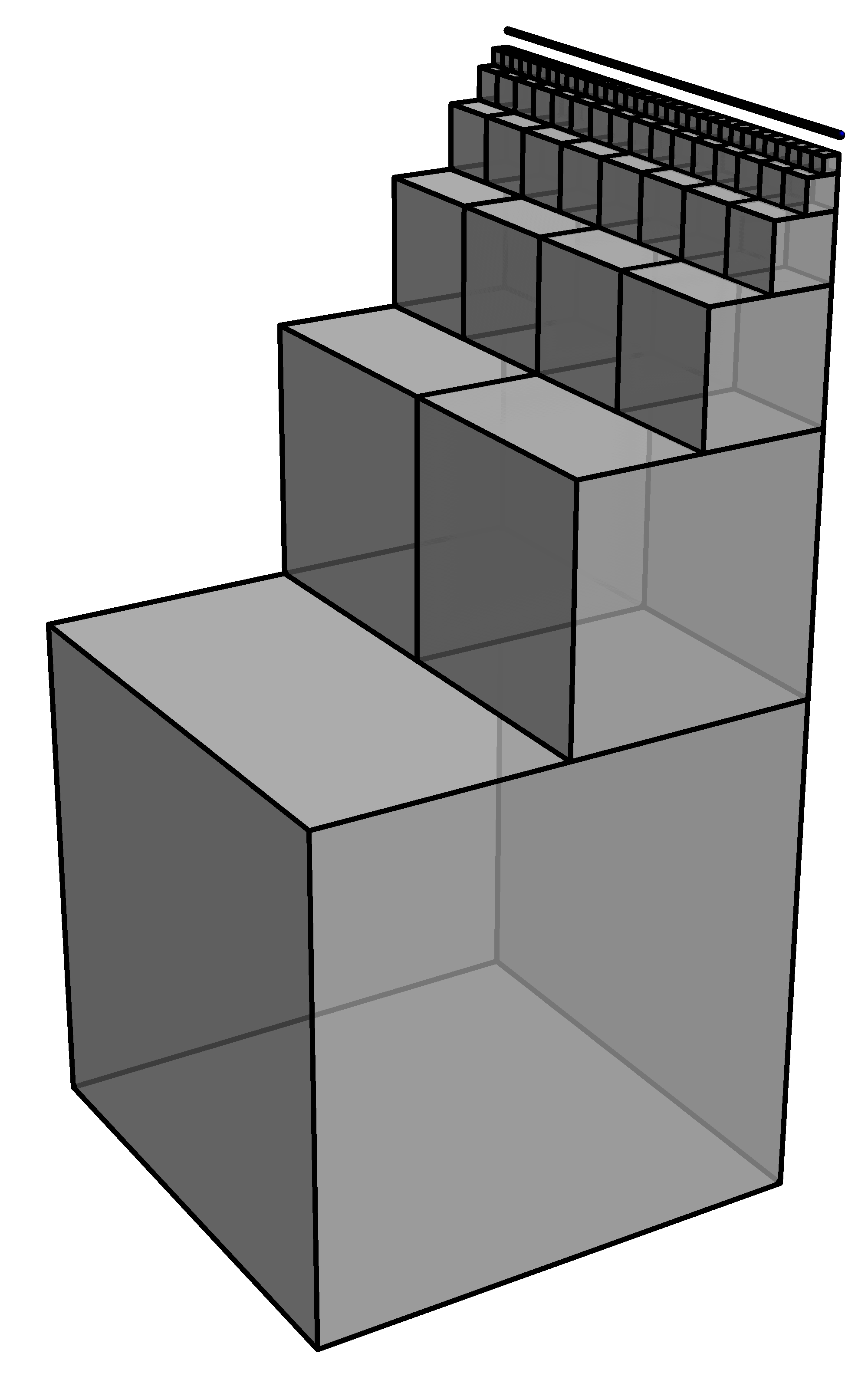
Figure 1: An infinite stack of cubes, also an admissible surface (which turns out to have infinite ℰq\mathcal{E}_{q}-energy for all q>2​m=4q>2m=4).

Let us first state the results precisely and then comment on the proofs and discuss the relations of this paper to existing research.

Remark 1.1.

Keep in mind, though, that all results stated in the introduction will be proved for a more general class 𝒜⁡(δ)\mathcal{A}(\delta) of admissible sets much larger than the preliminary class 𝒜\mathcal{A} defined above; see Section 2.3. To get a first impression of other admissible sets have a look at Figure 1.

Theorem 1.2 (Uniform Ahlfors regularity).

Assume that Σ∈𝒜\Sigma\in\mathcal{A} is an admissible mm-dimensional surface in ℝn{\mathbb{R}}^{n} with ℰq​(Σ)≤E\mathcal{E}_{q}(\Sigma)\leq E, q>2​mq>2m. There exists a constant a1=a1​(q,n,m)>0a_{1}=a_{1}(q,n,m)>0, depending only on q,nq,n and mm, such that

ℋm​(Σ∩B⁡(x,r))≥12​ω​(m)​rm\mathscr{H}^{m}(\Sigma\cap B(x,r))\geq\frac{1}{2}\omega(m)r^{m}

for all x∈Σx\in\Sigma and all radii

0<r<R1≡R1​(q,n,m,E):=a1E1/(q−2​m).0<r<R_{1}\equiv R_{1}(q,n,m,E):=\frac{a_{1}}{E^{1/(q-2m)}}\,.

(Here, and throughout the paper, B⁡(x,d)B(x,d) denotes the closed ball of radius dd centered at xx.)

In other words: if Σ∈𝒜\Sigma\in\mathcal{A} has finite energy for some q>2​mq>2m, then up to the length scale given by R1R_{1} – which depends only on the energy bound EE and the parameters m,n,qm,n,q, but not on Σ\Sigma itself – isolated thin fingers, narrow tubes, and the like cannot form on Σ\Sigma. The measure of the portion of Σ\Sigma inside the ball B⁡(x,r)B(x,r) is at least as large as half of the measure of the mm-dimensional equatorial cross-section of B⁡(x,r)B(x,r). A similar lower estimate on the Ahlfors regularity was proven by L. Simon for smooth two-dimensional surfaces with finite Willmore energy [30, Corollary 1.3]; see also the work of P. Topping [38] which even contains sharp lower bounds for the sum of local L2L^{2}-norm of the classic mean curvature and the area of the surface in a small ball. Mean curvature at a particular point xx on a smooth surface in ℝ3{\mathbb{R}}^{3} may be viewed as the arithmetic mean of minimal and maximal normal curvature at xx. Rtp−1R_{\rm tp}^{-1}, on the other hand, is a two-point function taking non-local interactions into account as well, but if one looks at the coalescent limits limy→xRtp−1​(x,y)\lim_{y\to x}R_{\rm tp}^{-1}(x,y) one obtains absolute values of intermediate normal curvatures at xx depending on the direction of approach as yy tends to xx (cf. [2, Section 3.2]). So, the local portion of our energy ℰq\mathcal{E}_{q} near xx may be regarded as another kind of averaging normal curvatures at xx, leading to density estimates as does the Willmore functional.

The next result gives a quantitative description of flatness of Σ\Sigma, in terms of the so-called β\beta-numbers introduced by P. Jones.

Theorem 1.3 (Uniform decay of β\beta-numbers).

Let Σ∈𝒜\Sigma\in\mathcal{A} be an admissible mm-dimensional surface in ℝn{\mathbb{R}}^{n} with ℰq​(Σ)<E\mathcal{E}_{q}(\Sigma)<E for some q>2​mq>2m. There exist two constants a2​(q,n,m)>0a_{2}(q,n,m)>0 and A2​(q,n,m)<∞A_{2}(q,n,m)\linebreak<\infty, both depending only on n,mn,m and qq, such that whenever the radius

d≤R2≡R2​(q,n,m,E):=a2​(q,n,m)E1/(q−2​m)d\leq R_{2}\equiv R_{2}(q,n,m,E):=\frac{a_{2}(q,n,m)}{E^{1/(q-2m)}} (1.3)

and the bound ε>0\varepsilon>0 satisfy the balance condition

ε4​m+q​d2​m−q≥A2​(q,n,m)​E,\varepsilon^{4m+q}d^{2m-q}\geq A_{2}(q,n,m)E\,, (1.4)

then we have

βΣ​(x,d):=infP∈G⁡(n,m)(supy∈B⁡(x,d)∩Σdist(y,x+P)d)≤ε,x∈Σ,\beta_{\Sigma}(x,d):=\inf_{P\in G(n,m)}\left(\sup_{y\in B(x,d)\cap\Sigma}\frac{\mathop{\rm dist}\nolimits(y,x+P)}{d}\right)\leq\varepsilon\,,\hskip 20.00003ptx\in\Sigma\,, (1.5)

where G⁡(n,m)G(n,m) denotes the Grassmannian of all mm-dimensional subspaces of ℝn{\mathbb{R}}^{n}.

Thus, for small dd we have

βΣ​(x,d)≲E1/(4​m+q)​dκ,κ:=q−2​mq+4​m>0.\beta_{\Sigma}(x,d)\lesssim E^{1/(4m+q)}d^{\kappa}\,,\hskip 20.00003pt\kappa:=\frac{q-2m}{q+4m}>0\,.

It is known that this condition alone does not suffice to conclude that Σ\Sigma is a topological manifold. D. Preiss, X. Tolsa and T. Toro [24], extending an earlier work of G. David, C. Kenig and T. Toro [7], study Reifenberg flat sets Σ\Sigma whose β\beta-numbers satisfy such estimates, see e.g. [24, Prop. 2.4] where it is proved that a decay bound for β\beta’s combined with Reifenberg flatness11 1 We do not define that condition here since we will not work with it directly; let us just mention that Reifenberg flatness means that the rescaled Hausdorff distance between Σ∩B⁡(x,d)\Sigma\cap B(x,d) and an mm-plane PP in B⁡(x,d)B(x,d) is uniformly controlled, and small. implies that Σ\Sigma must be a submanifold of class C1,κC^{1,\kappa}.

Since Σ∈𝒜\Sigma\in\mathcal{A} might, at least a priori, have transversal self–intersections, we do not have Reifenberg flatness here, and a quick direct use of the results of [7, 24] is impossible. However, we are able to use the energy estimates and the information given by Theorem 1.3 iteratively. Extending the ideas from our earlier work [34, Section 5] devoted to surfaces in ℝ3{\mathbb{R}}^{3}, we prove here that at every point x∈Σx\in\Sigma there exists the classic tangent plane Tx​ΣT_{x}\Sigma, and that the oscillation of tangent planes along Σ\Sigma satisfies uniform Hölder estimates. This implies that each Σ∈𝒜\Sigma\in\mathcal{A} with ℰq​(Σ)<∞\mathcal{E}_{q}(\Sigma)<\infty must be an embedded mm-dimensional manifold of class C1,κC^{1,\kappa}. Later on, working with graph patches of Σ\Sigma, we use slicing techniques and a bootstrap reasoning to improve and sharpen this information. The following theorem is the main result of this paper.

Theorem 1.4 (Geometric Sobolev–Morrey imbedding).

Let Σ∈𝒜\Sigma\in\mathcal{A} and ℰq​(Σ)<+∞\mathcal{E}_{q}(\Sigma)<+\infty for some q>2​mq>2m. Then Σ\Sigma is an embedded submanifold of class C1,μC^{1,\mu}, where μ=1−2​m/q\mu=1-2m/q.

In fact, there exist constants a3,A3>0a_{3},A_{3}>0, depending only on m,n,m,n, and qq, with the following property: For each x∈Σx\in\Sigma and each r≤R3=a3​ℰq​(Σ)1/(q−2​m)r\leq R_{3}=a_{3}\mathcal{E}_{q}(\Sigma)^{1/(q-2m)} there exists an mm-plane P∈G⁡(n,m)P\in G(n,m) and a function f:P≃ℝm→P⟂≃ℝn−mf\colon P\simeq{\mathbb{R}}^{m}\to P^{\perp}\simeq{\mathbb{R}}^{n-m} of class C1,μC^{1,\mu} such that

Σ∩B⁡(x,r)=Σ∩graph​f,\Sigma\cap B(x,r)=\Sigma\cap\mathrm{graph}\,f\,,

where graph​f⊂P×P⟂=ℝn\mathrm{graph}\,f\subset P\times P^{\perp}={\mathbb{R}}^{n} denotes the graph of ff, and

|∇f​(z)−∇f​(w)|≤A3​E​(x,r)1/q​|z−w|μ,z,w∈P∩B⁡(0,r),|\nabla f(z)-\nabla f(w)|\leq A_{3}E(x,r)^{1/q}|z-w|^{\mu},\hskip 20.00003ptz,w\in P\cap B(0,r), (1.6)

where

E⁡(x,r):=∫B⁡(x,r)∩Σ∫B⁡(x,r)∩Σ(1Rtp​(u,v))q​d​ℋm​(u)​d​ℋm​(v).E(x,r):=\int_{B(x,r)\cap\Sigma}\int_{B(x,r)\cap\Sigma}\left(\frac{1}{R_{\rm tp}(u,v)}\right)^{q}\,d\mathscr{H}^{m}(u)\,d\mathscr{H}^{m}(v)\,.

We believe that the exponent μ=1−2​m/q\mu=1-{2m}/{q}, strictly larger than κ=(q−2​m)/(q+4​m)\kappa=(q-2m)/(q+4m), is optimal here. It is clear that finiteness of ℰq\mathcal{E}_{q} does not lead to C2C^{2} regularity: consider a rotational cylinder closed with two hemispherical caps as an admissible surface Σ\Sigma of class C1,1C^{1,1} but not in C2C^{2}. For this particular surface inequality (1.6) is qualitatively optimal and, due to the factor E​(x,r)1/qE(x,r)^{1/q} and boundedness of 1/Rtp1/R_{\rm tp}, yields in fact Lipschitz estimates for the gradient of local graph representations of Σ\Sigma.

Please note two more things. First, the exponent μ=1−2​m/q\mu=1-2m/q is computed according to the recipe used in the classic Sobolev–Morrey imbedding theorem in the supercritical case. Here, the dimension of the domain of integration, i.e. of Σ×Σ\Sigma\times\Sigma, equals 2​m2m. We have μ→1\mu\to 1 as q→∞q\to\infty; for two-dimensional surfaces, the limiting case q=∞q=\infty has been treated earlier in our papers [32] and [33].

Second, what we have learnt about Σ\Sigma is not limited to embeddedness and purely qualitative C1,μC^{1,\mu} estimates. It is clear that the bounds given by Theorem 1.4 are uniform in any class of surfaces with uniformly bounded energy ℰq\mathcal{E}_{q}. In other words, if 𝒦={Σi:i∈I}⊂𝒜\mathcal{K}=\{\Sigma_{i}\colon i\in I\}\subset\mathcal{A} satisfies

supi∈Iℰq​(Σi)≤M<∞,\sup_{i\in I}\mathcal{E}_{q}(\Sigma_{i})\leq M<\infty\,, (1.7)

then we can find two constants A,δ>0A,\delta>0, depending only on M,m,nM,m,n and qq, such that each Σi∩B⁡(x,δ)\Sigma_{i}\cap B(x,\delta), where i∈Ii\in I and x∈Σix\in\Sigma_{i}, is obtained by a rigid motion of ℝn{\mathbb{R}}^{n} from a graph of a function f:ℝm→(ℝm)⟂≃ℝn−mf\colon{\mathbb{R}}^{m}\to({\mathbb{R}}^{m})^{\perp}\simeq{\mathbb{R}}^{n-m} which satisfies the uniform estimate ‖f‖C1,μ≤A\|f\|_{C^{1,\mu}}\leq A, no matter how i∈Ii\in I and x∈Σix\in\Sigma_{i} have been chosen. Thus, a uniform upper bound on ℰq\mathcal{E}_{q} allows us to fix a uniform size of charts for all Σi∈𝒦\Sigma_{i}\in\mathcal{K}, and forces the equicontinuity of gradients of local graph representations of the surfaces Σi\Sigma_{i}. In a forthcoming paper [36] we show how to use this idea to obtain finiteness theorems for classes of C1C^{1} embedded manifolds Σi\Sigma_{i} in ℝn{\mathbb{R}}^{n} satisfying a volume constraint and a uniform energy bound (1.7).

We do not know what happens in the critical case q=2​mq=2m. Let us mention here one plausible conjecture that we cannot prove at this stage.

Conjecture 1.5.

Every immersed mm-dimensional C1C^{1}-manifold in Σ⊂ℝn\Sigma\subset{\mathbb{R}}^{n} with finite ℰ2​m\mathcal{E}_{2m}-energy is embedded.

Another, probably more difficult, question that we cannot handle at present is the following: how regular are the minimizers of ℰq\mathcal{E}_{q} (say, with upper bounds for the total measure, to prevent the decrease of energy caused by rescaling) in isotopy classes of C1C^{1} embedded manifolds? Are they C1,1C^{1,1} (this is optimal for ideal links [5] – corresponding to the case q=∞q=\infty in dimensions n=3n=3 and m=1m=1 – where contact phenomena are present)? Or maybe C∞C^{\infty}, as minimizers of a Möbius invariant knot energy in [9], [14]; see also [25], [26]? In addition, S. Blatt [3] characterized all curves with finite Möbius energy as embeddings in certain Sobolev-Slobodeckiĭ classes; such a characterization of finite energy submanifolds for the tangent-point energy ℰq\mathcal{E}_{q} is presently not known.

Our interest in this topic has been triggered by several factors. They include manifold applications of Menger curvature in harmonic analysis and geometric measure theory (see e.g. the survey articles of P. Mattila [21], [22], G. David [6] and X. Tolsa [37], and the literature cited therein, including J.C. Léger [18] and the relation between 11-rectifiability and L2L^{2}-integrability of Menger curvature). There are also works of different origin, investigating another geometric concept, the so-called global curvature introduced by Gonzalez and Maddocks [12]. The second author of the present paper took part in laying out the strict mathematical foundations for global curvature of rectifiable loops and its variational applications to elastic curves and rods with positive thickness; see [13], [27], [28], [29], [10], [11]. Part of this work, in turn, has been a starting point for our subsequent joint research devoted to various energies that, roughly speaking, interpolate between global curvature and Menger curvature. Finiteness of these energies; see e.g. [31], [34], [35], analogously to the case that we consider here, leads to an increase of regularity, to compactness effects, and yields a tool to control the amount of bending of non-smooth objects in purely geometric terms.22 2 In [35] we treat the toy case m=1m=1 of the present paper, along with a few knot-theoretic applications of ℰq\mathcal{E}_{q} for curves. The novelty in the present paper is that we work in full generality, overcoming the difficulty that both the dimension and the codimension may be arbitrary. In an ongoing research [16, 17] S. Kolasiński obtains analogues of our results for basically the same admissible class of surfaces that we consider here, but for a different integral energy, defined as an (m+2)(m+2)-fold integral (with respect to ℋm\mathscr{H}^{m}) over the set of all simplices with vertices on Σ\Sigma, directly extending our results in [34] to surfaces of arbitrary dimension and codimension.

Closely related research includes also G. Lerman and J.T. Whitehouse [19], [20], who investigate a number of ingenious high-dimensional curvatures of Menger type and obtain rectifiability criteria for dd-dimensional subsets of Hilbert spaces. Last but not least, the deep and classic paper of W. Allard [1] sets forth a regularity theory for mm-dimensional varifolds whose first variation (roughly: the distributional counterpart of mean curvature) is in LpL^{p} for some p>mp>m. Our regularity results bear some resemblance to his Theorem 8.1. There are many differences, though, that remain to be fully understood. It is clear that without some extra topological assumptions on Σ\Sigma finiteness of (1.1) cannot lead to the conclusion that Σ\Sigma is locally (on a scale depending only on the energy!) homeomorphic to a disc; one could punch an arbitrary number of ‘holes’ in a smooth surface and this would just decrease the energy we work with. In Allard’s case, once we fix a ball where appropriate density estimates hold and the weight ‖V‖\|V\| of the varifold VV is close to the Hausdorff measure of a disk, then the ‘lack of holes’ is built into his assumption on the first variation δ​V\delta V of VV. On the other hand, ℰq\mathcal{E}_{q} – as a non-local energy in contrast to the locally defined distributional mean curvature – averages over all global tangent-point interactions, which leads to self-avoidance and control over topology of the given surface. Admissible sets with finite ℰq\mathcal{E}_{q}-energy are differentiable manifolds, which Allard’s result cannot guarantee for varifolds with distributional mean curvature in LpL^{p}, p>mp>m: there is a remaining (small) singular set, such that there is no control on the topology of the support of the varifold measure. To possibly bridge the apparent gap between Allard’s work and our results we should note that versions of ℰq\mathcal{E}_{q} can be defined for general mm-dimensional varifolds VV, via double integrals: the integrand 1/Rtp1/R_{\rm tp} can be treated as a function on points and planes. It is an intriguing question whether finiteness of such integrals for some qq’s lead to rectifiability criteria or to an improved regularity in the case of varifolds.

Let us now informally sketch the main thread of our reasoning, and describe the organization of the paper in more detail. We want to exclude self intersections and to have a quantitative description of flatness; for this, Theorem 1.3 would be a good starting point. The main idea behind its proof is pretty straightforward: if the β\beta-numbers were too large, i.e. if x∈Σx\in\Sigma but Σ∩B⁡(x,d)\Sigma\cap B(x,d) were not confined to a narrow tube Bε​d​(x+P)B_{\varepsilon d}(x+P) around some affine mm-plane x+Px+P, then, a simple argument shows that we would have two much smaller balls B1,B2⊂BB_{1},B_{2}\subset B, say with

diamB1=diamB2≈ε2​d\mathop{\rm diam}\nolimits B_{1}=\mathop{\rm diam}\nolimits B_{2}\approx\varepsilon^{2}d

such that for all y∈Σ∩B2y\in\Sigma\cap B_{2} and a nonzero proportion of z∈Σ∩B1z\in\Sigma\cap B_{1} the distance dist(y,z+Tz​Σ)\mathop{\rm dist}\nolimits(y,z+T_{z}\Sigma) would be comparable to ε​d\varepsilon d. This yields 1/Rtp​(y,z)≳ε/d1/R_{\rm tp}(y,z)\gtrsim\varepsilon/d, and a lower bound for the energy follows easily, leading to a contradiction, if the B1,B2B_{1},B_{2} and the bound for the β\beta’s are chosen in a suitable way which happens to be precisely the balance condition (1.4). There is only one serious catch here: in order to make the resulting estimate uniform, and to be able to iterate it later on, we must guarantee that

ℋm​(Σ∩Br)≥c⋅rmfor all r<r0=r0​(energy),\mathscr{H}^{m}(\Sigma\cap B_{r})\geq c\cdot r^{m}\hskip 20.00003pt\mbox{for all $r<r_{0}=r_{0}(\text{energy})$,}

with some absolute constant cc. And we want both r0r_{0} and cc independent of a particular Σ\Sigma.

For this, we need Theorem 1.2 which serves as the backbone for all the later constructions and estimates of the paper. The overall idea here is somewhat similar to an analogous result in our work [34] on Menger curvature for surfaces in ℝ3{\mathbb{R}}^{3}. The main difference, however, leading to crucial difficulties, is that the codimension of Σ\Sigma may be arbitrary.

The proof of Theorem 1.2 has two stages. First, for a fixed generic point x∈Σx\in\Sigma and all radii rr below a stopping distance ds​(x)d_{s}(x), we control the size of projections of Σ∩B⁡(x,r)\Sigma\cap B(x,r) onto some mm-plane H⁡(r)H(r) (which may vary as rr varies). Here, topology comes into play. To grasp the essence of our idea, it is convenient to think of Σ=M1∪…∪MN\Sigma=M_{1}\cup\ldots\cup M_{N} as in Example (i) at the beginning of the introduction. For x∈Mi∖⋃j≠iMjx\in M_{i}\setminus\bigcup_{j\not=i}M_{j} and for infinitesimally small radii rr we start with the tangent planes P=Tx​MiP=T_{x}M_{i}, and note that small (n−m−1)(n-m-1)-spheres that are perpendicular to Tx​MiT_{x}M_{i} are nontrivially linked with MiM_{i}. Then, for a sequence of growing radii ρ\rho, we rotate PP if necessary by a controlled angle to a new position PρP_{\rho} in order to keep the projections large. At the same time, we construct a growing connected excluded region SρS_{\rho} which does not contain any point of Σ\Sigma in its interior. The size of the projections is controlled via a topological argument, involving the homotopy invariance of the linking number mod 2 of submanifolds. The construction stops at some stopping distance r=ds​(x)r=d_{s}(x) , and yields another point y∈Σy\in\Sigma with |y−x|≈ds​(x)|y-x|\approx d_{s}(x) and two smaller balls B⁡(x,c​ds​(x))B(x,cd_{s}(x)), B⁡(y,c​ds​(x))B(y,cd_{s}(x)), where c∈(0,1)c\in(0,1) is an explicit absolute constant, such that

1Rtp​(z,w)≳1ds​(x)\frac{1}{R_{\rm tp}(z,w)}\gtrsim\frac{1}{d_{s}(x)}

for all w∈B⁡(y,c​ds​(x))w\in B(y,cd_{s}(x)) and a significant proportion of z∈B⁡(x,c​ds​(x))z\in B(x,cd_{s}(x)). In the second stage we use the energy bounds to show that d⁡(Σ):=infx∈Σds​(x)d(\Sigma):=\inf_{x\in\Sigma}d_{s}(x) is positive and satisfies d⁡(Σ)≥R1d(\Sigma)\geq R_{1}, where R1R_{1} is the uniform constant given in Theorem 1.2. The details of that part are given in Section 4; see Lemma 4.2, Lemma 4.3 and their corollaries.

Sections 2 and 3 contain all the necessary prerequisites and are included for the sake of completeness. In Section 2 we gather elementary estimates of angles between planes spanned by nearby almost orthogonal bases, and introduce the class of admissible sets whose definition is designed so that the above sketchy idea can be made precise. In Section 3 we explain how the linking number mod 2 can be used for elements of 𝒜\mathcal{A}, providing specific statements (and short proofs) for sake of further reference.

Once Theorem 1.2 is proved, we use the Hausdorff convergence of excluded regions defined for generic points x∈Σx\in\Sigma to obtain a corollary which, roughly speaking, ascertains that for every x∈Σx\in\Sigma and r≤R1r\leq R_{1} there is some plane H=Hx,r∈G⁡(n,m)H=H_{x,r}\in G(n,m) such that Σ∩B⁡(x,r)\Sigma\cap B(x,r) has large projection onto HH and is contained either in B⁡(x,r/2)B(x,r/2) (where, a priori, at this stage of the reasoning, Σ\Sigma might behave in a pretty wild way) or in a narrow tubular region Bδ​(x+H)B_{\delta}(x+H), for some specific constant δ≪1\delta\ll 1. A use of energy bounds yields now Theorem 1.3, and an iterative argument implies that in fact Σ\Sigma must locally be a C1,κC^{1,\kappa} graph. All this is done in Section 5. Embeddedness of Σ\Sigma is established here, too.

Finally, in Section 6, we prove Theorem 1.4 and sharpen the Hölder bounds. To this end, we show that if Σ∩B\Sigma\cap B is a graph of f∈C1,κf\in C^{1,\kappa}, then ∇f\nabla f satisfies an improved estimate,

|∇f​(a1)−∇f​(a2)|≤2​Φ∗​(|a1−a2|/N)+C​E1/q​|a1−a2|μ,|\nabla f(a_{1})-\nabla f(a_{2})|\leq 2\Phi^{\ast}(|a_{1}-a_{2}|/N)+C\,E^{1/q}\,|a_{1}-a_{2}|^{\mu}, (1.8)

where Φ∗​(s)\Phi^{\ast}(s) stands for the supremum of oscillations of ∇f\nabla f over all possible balls of radius ss, and EE is the portion of energy coming from some ball containing a1,a2a_{1},a_{2}. The point is that (1.8) holds for some N=N⁡(q)≫1N=N(q)\gg 1, so that for f∈C1,κf\in C^{1,\kappa} the first term of the right hand side can be viewed as an unimportant, small scale perturbation. The main idea behind (1.8) is that when the integral average of (1/Rtp)q(1/R_{\rm tp})^{q} is bounded by KK, then there are numerous points uiu_{i} in small balls around the aia_{i}, i=1,2i=1,2, where (1/Rtp)q≲K(1/R_{\rm tp})^{q}\lesssim K. A geometric argument implies that for such points |∇f​(u1)−∇f​(u2)||\nabla f(u_{1})-\nabla f(u_{2})| can be controlled by the second term in the right hand side of (1.8), and a routine iterative reasoning, with a certain Morrey–Campanato flavour, allows us to get rid of the 2​Φ∗2\Phi^{\ast} and finish the whole proof.

Acknowledgement.  The authors would like to thank the Deutsche Forschungsgemeinschaft, Polish Ministry of Science and Higher Education, and the Alexander von Humboldt Foundation, for generously supporting this research. Substantial parts of this work have been written while the first author has been staying at the RWTH Aachen University in the fall of 2009; he is very grateful to his German colleagues for their hospitality.

2 Bases, projections, angle estimates, and the class of admissible sets

2.1 Balls, slabs, planes

We write B⁡(x,r)B(x,r) to denote the closed ball in ℝn{\mathbb{R}}^{n}, with center xx and radius r>0r>0. The volume of the unit ball in ℝk{\mathbb{R}}^{k} is denoted by ω⁡(k)\omega(k).

For a closed set FF in ℝn{\mathbb{R}}^{n} we set

Uδ​(F):={x∈ℝn:dist(x,F)<δ},δ>0.U_{\delta}(F):=\{x\in{\mathbb{R}}^{n}\,\colon\,\mathop{\rm dist}\nolimits(x,F)<\delta\},\hskip 20.00003pt\delta>0.

G⁡(n,m)G(n,m) denotes the Grassmannian of all mm-dimensional linear subspaces of ℝn{\mathbb{R}}^{n}. If P∈G⁡(n,m)P\in G(n,m), then πP\pi_{P} denotes the orthogonal projection of ℝn{\mathbb{R}}^{n} onto PP, and QPQ_{P} is the orthogonal projection onto P⟂∈G⁡(n,n−m)P^{\perp}\in G(n,n-m).

For two planes P1,P2∈G⁡(n,m)P_{1},P_{2}\in G(n,m) we define their distance (or angle)

OPEN<)⁡(P1,P2)≡d⁡(P1,P2):=‖πP1−πP2‖,\mathop{\mbox{$<\!\!\!)$}}\nolimits(P_{1},P_{2})\equiv d(P_{1},P_{2}):=\|\pi_{P_{1}}-\pi_{P_{2}}\|\,,

where the right hand side is the usual norm of the linear map πP1−πP2:ℝn→ℝn\pi_{P_{1}}-\pi_{P_{2}}\colon{\mathbb{R}}^{n}\to{\mathbb{R}}^{n}. The Grassmannian G⁡(n,m)G(n,m) equipped with this metric is compact.

Finally, we use the following variant of P. Jones’ beta-numbers (see David’s and Semmes’ monograph [8, Chapter 1, Sec. 1.3] for a discussion):

βΣ​(x,r):=infL∈G⁡(n,m)(supy∈Σ∩B⁡(x,r)dist(y,x+L)r),x∈Σ,r>0.\beta_{\Sigma}(x,r):=\inf_{L\in G(n,m)}\left(\sup_{y\in\Sigma\cap B(x,r)}\ \frac{\mathop{\rm dist}\nolimits(y,x+L)}{r}\right),\hskip 20.00003ptx\in\Sigma,\hskip 10.00002ptr>0. (2.1)

2.2 Nearby planes: bases, projections, angle estimates

Throughout most of the paper, we shall work with estimates of various geometric quantities related to two planes in G⁡(n,m)G(n,m) that form a small angle. For sake of further reference, we gather here several such estimates. We also fix specific constants (which in all cases are far from being optimal) that are needed later, in more involved computations in Sections 4–6. All proofs are elementary, but we provide them to make the exposition complete.

Lemma 2.1.

Assume that a,b>0a,b>0 and a sequence of nonnegative numbers sks_{k} satisfies s1≤1s_{1}\leq 1,

sk+1≤a​k+b​∑j=1ksj,k≥1.s_{k+1}\leq ak+b\sum_{j=1}^{k}s_{j},\hskip 20.00003ptk\geq 1.

Then for each A≥1+max⁡(2​a,2​b)A\geq 1+\max(2a,2b) we have sk<Aks_{k}<A^{k}, k=1,2​…k=1,2\ldots.

Proof. One proceeds by induction. Clearly, for k=1k=1 we just need s1≤1<As_{1}\leq 1<A. For each A>1A>1 the recursive condition for sk+1s_{k+1} yields, under the inductive hypothesis,

sk+1<a​k+A​bA−1​(Ak−1)s_{k+1}<ak+\frac{Ab}{A-1}(A^{k}-1) (2.2)

Now, A≥1+max⁡(2​a,2​b)A\geq 1+\max(2a,2b) guarantees that 2​a​k<(1+2​a)k≤Ak≤Ak+12ak<(1+2a)^{k}\leq A^{k}\leq A^{k+1} andbA−1≤12\frac{b}{A-1}\leq\frac{1}{2}. Thus, (2.2) yields 2​sk+1<Ak+1+Ak+1−A<2​Ak+12s_{k+1}<A^{k+1}+A^{k+1}-A<2A^{k+1}. □\Box

Lemma 2.2.

If X,Y∈G⁡(n,l)X,Y\in G(n,l) have orthonormal bases (ej)⊂X(e_{j})\subset X and (fj)⊂Y(f_{j})\subset Y such that |ej−fj|≤α|e_{j}-f_{j}|\leq\alpha for each j=1,…,lj=1,\ldots,l, then 𝑂𝑃𝐸𝑁<)⁡(X,Y)≤2​l​α\mathop{\mbox{$<\!\!\!)$}}\nolimits(X,Y)\leq 2l\alpha.

Proof. Take an arbitrary unit vector v∈ℝnv\in{\mathbb{R}}^{n} and estimate |πX​(v)−πY​(v)||\pi_{X}(v)-\pi_{Y}(v)|, expressing both projections in orthonormal bases (ej)(e_{j}) and (fj)(f_{j}). □\Box

Lemma 2.3.

Assume that 1≤l≤m≤n1\leq l\leq m\leq n. If e1,…,ele_{1},\ldots,e_{l} is an orthonormal basis of a subspace X∈G⁡(n,l)X\in G(n,l) and h1,…,hl∈ℝnh_{1},\ldots,h_{l}\in{\mathbb{R}}^{n} satisfy |hi−ei|<ε<ε1:=10−1​(10m+1)−1|h_{i}-e_{i}|<\varepsilon<\varepsilon_{1}:=10^{-1}(10^{m}+1)^{-1}, then (hi)i=1,…,l(h_{i})_{i=1,\ldots,l} are linearly independent. Moreover, the Gram-Schmidt orthogonalization process

ui:=vi|vi|,wherev1=h1,vk+1=hk+1−∑j=1k⟨hk+1,vj⟩|vj|2​vj,k+1≤l,u_{i}:=\frac{v_{i}}{|v_{i}|},\hskip 20.00003pt\mbox{where}\hskip 10.00002ptv_{1}=h_{1},\hskip 10.00002ptv_{k+1}=h_{k+1}-\sum_{j=1}^{k}\frac{\langle h_{k+1},v_{j}\rangle}{|v_{j}|^{2}}v_{j}\,,\hskip 10.00002ptk+1\leq l,

yields vectors vi,uiv_{i},u_{i} (i=1,…,l)(i=1,\ldots,l) that satisfy

|vk−hk|<10kε,||vk|−1|<(10k+1)ε<110for all k=1,…,l,\displaystyle|v_{k}-h_{k}|<10^{k}\varepsilon,\hskip 20.00003pt\bigl||v_{k}|-1\bigr|<(10^{k}+1)\varepsilon<\frac{1}{10}\hskip 10.00002pt\mbox{for all $k=1,\ldots,l$,} (2.3)
|uk−ek|<c1​ε<12for all i=1,…,l,\displaystyle|u_{k}-e_{k}|<c_{1}\varepsilon<\frac{1}{2}\hskip 10.00002pt\mbox{for all $i=1,\ldots,l$,} (2.4)

where c1:=2​(10m+1)c_{1}:=2(10^{m}+1). If Y=span⁡(h1,…,hl)Y=\mathrm{span}\,(h_{1},\ldots,h_{l}), then

OPEN<)⁡(X,Y)≤c2​ε,\mathop{\mbox{$<\!\!\!)$}}\nolimits(X,Y)\leq c_{2}\varepsilon\,, (2.5)

with c2:=2​m​c1=4​m​(10m+1)c_{2}:=2mc_{1}=4m(10^{m}+1).

Proof. As |hj−ej|<ε|h_{j}-e_{j}|<\varepsilon for all jj, we have |⟨hi,hj⟩−⟨ei,ej⟩|<3​ε|\langle h_{i},h_{j}\rangle-\langle e_{i},e_{j}\rangle|<3\varepsilon. Therefore, |⟨hk+1,vj⟩|<3​ε+(1+ε)​|hj−vj||\langle h_{k+1},v_{j}\rangle|<3\varepsilon+(1+\varepsilon)|h_{j}-v_{j}| for j=1,…,kj=1,\ldots,k and k≤l−1k\leq l-1. Using this observation, one proves (2.3) by induction; assuming (2.3) for kk and all j<kj<k, we obtain

|vk+1−hk+1|\displaystyle|v_{k+1}-h_{k+1}| ≤\displaystyle\leq ∑j=1k|⟨hk+1,vj⟩||vj|<∑j=1k3​ε+(1+ε)​|vj−hj||vj|\displaystyle\sum_{j=1}^{k}\frac{|\langle h_{k+1},v_{j}\rangle|}{|v_{j}|}<\sum_{j=1}^{k}\frac{3\varepsilon+(1+\varepsilon)|v_{j}-h_{j}|}{|v_{j}|}
<\displaystyle< 109​3​k​ε+119​∑j=1k10j​ε<10k+1​ε,\displaystyle\frac{10}{9}3\,k\varepsilon+\frac{11}{9}\sum_{j=1}^{k}10^{j}\varepsilon<10^{k+1}\varepsilon,

where the last inequality follows from elementary computations (the estimate is not sharp). This yields the first part of (2.3) for k+1k+1; the second one follows from the triangle inequality.

In particular, we also have dist(hk+1,span(h1,…,hk))=|vk+1|>0\mathop{\rm dist}\nolimits\bigl(h_{k+1},\mathop{\rm span}\nolimits(h_{1},\ldots,h_{k})\bigr)=|v_{k+1}|>0, and therefore h1,…,hlh_{1},\ldots,h_{l} are linearly independent.

Setting ui:=vi/|vi|u_{i}:=v_{i}/|v_{i}|, we easily conclude the proof of the whole lemma. (To check inequality (2.5), apply Lemma 2.2 and note that l≤ml\leq m.) □\Box

Lemma 2.4.

Let ε1\varepsilon_{1} be the constant defined in Lemma 2.3 above. Assume that

  1. (i)

    there exist orthonormal e1,…,em∈ℝne_{1},\ldots,e_{m}\in{\mathbb{R}}^{n} such that hi∈Bn​(ei,δ)h_{i}\in B^{n}(e_{i},\delta) for i=1,…,mi=1,\ldots,m, and δ<ε1/2\delta<\varepsilon_{1}/2;

  2. (ii)

    wi∈Bn​(hi,ε)w_{i}\in B^{n}(h_{i},\varepsilon) for all i=1,…,mi=1,\ldots,m, and ε<ε1/2\varepsilon<\varepsilon_{1}/2.

Then the subspaces H=span(h1,…,hm)H=\mathop{\rm span}\nolimits(h_{1},\ldots,h_{m}) and W=span(w1,…,wm)W=\mathop{\rm span}\nolimits(w_{1},\ldots,w_{m}) belong to G⁡(n,m)G(n,m), and we have 𝑂𝑃𝐸𝑁<)⁡(H,W)≤c3​ε\mathop{\mbox{$<\!\!\!)$}}\nolimits(H,W)\leq c_{3}\varepsilon with c3=14​m⋅20mc_{3}=14m\cdot 20^{m}.

Proof. It follows from Lemma 2.3 that dimH=dimW=m\dim H=\dim W=m. We use again the Gram-Schmidt algorithm and set v1=h1v_{1}=h_{1}, u1=w1u_{1}=w_{1},

vk+1=hk+1−∑j=1k⟨hk+1,vj⟩|vj|2​vj,uk+1=wk+1−∑j=1k⟨wk+1,uj⟩|uj|2​uj,k+1≤m.\hskip 20.00003ptv_{k+1}=h_{k+1}-\sum_{j=1}^{k}\frac{\langle h_{k+1},v_{j}\rangle}{|v_{j}|^{2}}v_{j}\,,\hskip 20.00003ptu_{k+1}=w_{k+1}-\sum_{j=1}^{k}\frac{\langle w_{k+1},u_{j}\rangle}{|u_{j}|^{2}}u_{j}\,,\hskip 20.00003ptk+1\leq m.

Then, viv_{i} and uiu_{i} form orthogonal bases of HH and WW, respectively. Inequality (2.3) yields t−1<|ui|,|vi|<tt^{-1}<|u_{i}|,|v_{i}|<t with t=10/9t=10/9. We now show that si=ε−1​|ui−vi|s_{i}=\varepsilon^{-1}|u_{i}-v_{i}| satisfies the assumptions of Lemma 2.1 with a=1a=1 and b=8b=8. For k=1k=1 we have s1=ε−1​|h1−w1|<1s_{1}=\varepsilon^{-1}|h_{1}-w_{1}|<1.

Let ϕ⁡(x)=|x|−2​x\phi(x)=|x|^{-2}x. For all x,yx,y in the annulus {t−1≤|z|≤t}\{t^{-1}\leq|z|\leq t\} we have |ϕ⁡(x)|≤t|\phi(x)|\leq t and, for x≠yx\not=y,

|ϕ⁡(x)−ϕ⁡(y)|\displaystyle|\phi(x)-\phi(y)| ≤\displaystyle\leq |x−y||x|2+|y||1|x|2−1|y|2|≤t2​|x−y|+t​|∫|x||y|2τ3​𝑑τ|\displaystyle\frac{|x-y|}{|x|^{2}}+|y|\biggl|\frac{1}{|x|^{2}}-\frac{1}{|y|^{2}}\biggr|\leq t^{2}|x-y|+t\biggl|\int_{|x|}^{|y|}\frac{2}{\tau^{3}}\,d\tau\biggr|
≤\displaystyle\leq t2​(1+2​t2)​|x−y|< 5​|x−y|,as t=10/9.\displaystyle t^{2}(1+2t^{2})|x-y|\ <\ 5|x-y|\,,\hskip 20.00003pt\mbox{as $t=10/9$.}

Thus, since wj,uj,vj∈{t−1≤|z|≤t}w_{j},u_{j},v_{j}\in\{t^{-1}\leq|z|\leq t\}, we obtain

|uk+1−vk+1|\displaystyle|u_{k+1}-v_{k+1}| ≤\displaystyle\leq |hk+1−wk+1|+|∑j=1k⟨hj,ϕ⁡(vj)⟩​vj−⟨wj,ϕ⁡(uj)⟩​uj|\displaystyle|h_{k+1}-w_{k+1}|+\biggl|\sum_{j=1}^{k}\langle h_{j},\phi(v_{j})\rangle v_{j}-\langle w_{j},\phi(u_{j})\rangle u_{j}\biggl|
≤\displaystyle\leq ε+∑j=1k(ε+t2​(|ϕ⁡(vj)−ϕ⁡(uj)|+|vj−uj|))≤ε+∑j=1k(ε+6​t2​|vj−uj|).\displaystyle\varepsilon+\sum_{j=1}^{k}\Bigl(\varepsilon+t^{2}\bigl(|\phi(v_{j})-\phi(u_{j})|+|v_{j}-u_{j}|\bigr)\Bigr)\ \leq\ \varepsilon+\sum_{j=1}^{k}\Bigl(\varepsilon+6t^{2}|v_{j}-u_{j}|\Bigr)\,.

Hence,

sk+1=ε−1​|uk+1−vk+1|≤(k+1)+b​∑j=1ksjs_{k+1}=\varepsilon^{-1}|u_{k+1}-v_{k+1}|\leq(k+1)+b\sum_{j=1}^{k}s_{j}

for each b≥6​t2b\geq 6t^{2}, in particular for b=8b=8. Therefore certainly sk≤20ks_{k}\leq 20^{k}, k=1,…,mk=1,\ldots,m, by Lemma 2.1. Keeping in mind that t−1=910≤|uj|,|vj|≤109=tt^{-1}=\frac{9}{10}\leq|u_{j}|,|v_{j}|\leq\frac{10}{9}=t, we obtain

|uj|uj|−vj|vj||=||uj|​ϕ​(uj)−|vj​|ϕ⁡(vj)|<6​t|uj−vj|<7⋅20m​ε.\biggl|\frac{u_{j}}{|u_{j}|}-\frac{v_{j}}{|v_{j}|}\biggr|=\bigl||u_{j}|\phi(u_{j})-|v_{j}|\phi(v_{j})\bigr|<6t|u_{j}-v_{j}|<7\cdot 20^{m}\varepsilon\,.

The inequality OPEN<)⁡(H,W)≤c3​ε\mathop{\mbox{$<\!\!\!)$}}\nolimits(H,W)\leq c_{3}\varepsilon follows now from Lemma 2.2. □\Box

The next two lemmata are concerned with the set

S(H1,H2):={y∈ℝn:dist(y,Hi)≤1for i=1,2},S(H_{1},H_{2}):=\{y\in{\mathbb{R}}^{n}\,\colon\mathop{\rm dist}\nolimits(y,H_{i})\leq 1\hskip 10.00002pt\mbox{for $i=1,2$}\}, (2.6)

where H1≠H2∈G⁡(n,m)H_{1}\not=H_{2}\in G(n,m) form a small angle so that πH1\pi_{H_{1}} restricted to H2H_{2} is bijective. Since {y∈ℝn:dist(y,Hi)≤1}\{y\in{\mathbb{R}}^{n}\,\colon\mathop{\rm dist}\nolimits(y,H_{i})\leq 1\} is convex, closed and centrally symmetric33 3 The term central symmetry is used here for central symmetry with respect to 00 in ℝn{\mathbb{R}}^{n}. for each i=1,2i=1,2, we immediately obtain the following:

Lemma 2.5.

S⁡(H1,H2)S(H_{1},H_{2}) is a convex, closed and centrally symmetric set in ℝn{\mathbb{R}}^{n}; πH1​(S⁡(H1,H2))\pi_{H_{1}}(S(H_{1},H_{2})) is a convex, closed and centrally symmetric set in H1≅ℝmH_{1}\cong{\mathbb{R}}^{m}.

The next lemma and its corollary provide a key tool for bootstrap estimates in Section 6.

Lemma 2.6.

Let ε1>0\varepsilon_{1}>0 and c2>0c_{2}>0 denote the constants defined in Lemma 2.3. If H1,H2∈G⁡(n,m)H_{1},H_{2}\in G(n,m) satisfy 0<𝑂𝑃𝐸𝑁<)⁡(H1,H2)=α<ε10<\mathop{\mbox{$<\!\!\!)$}}\nolimits(H_{1},H_{2})=\alpha<\varepsilon_{1}, then there exists an (m−1)(m-1)-dimensional subspace W⊂H1W\subset H_{1} such that

πH1​(S⁡(H1,H2))⊂{y∈H1:dist(y,W)≤5​c2/α}.\pi_{H_{1}}\bigl(S(H_{1},H_{2})\bigr)\subset\{y\in H_{1}\colon\mathop{\rm dist}\nolimits(y,W)\leq 5c_{2}/\alpha\}\,.

Proof. Let H:=H1∩H2H:=H_{1}\cap H_{2}; we have k:=dimH<mk:=\dim H<m. For i=1,2i=1,2 set Xi={x∈Hi:x⟂H}X_{i}=\{x\in H_{i}\,\colon x\perp H\}. Then, HiH_{i} is the orthogonal sum of HH and XiX_{i}. Let X:=X1⊕X2X:=X_{1}\oplus X_{2}; by construction, X⟂HX\perp H. Finally, let LL be the orthogonal complement of H⊕X=H1⊕H2H\oplus X=H_{1}\oplus H_{2} in ℝn{\mathbb{R}}^{n}, so that ℝn{\mathbb{R}}^{n} is equal to H⊕X⊕LH\oplus X\oplus L, and the spaces H,X,LH,X,L are pairwise orthogonal. It is now easy to see, directly by definition, that OPEN<)⁡(H1,H2)=OPEN<)⁡(X1,X2)\mathop{\mbox{$<\!\!\!)$}}\nolimits(H_{1},H_{2})=\mathop{\mbox{$<\!\!\!)$}}\nolimits(X_{1},X_{2}).

Step 1. We shall first show that there exists a vector x1∈X1x_{1}\in X_{1} such that

|x1|=5​c2/α,x1∉πH1​(S⁡(H1,H2)).|x_{1}|=5c_{2}/\alpha,\hskip 20.00003ptx_{1}\not\in\pi_{H_{1}}(S(H_{1},H_{2}))\,. (2.7)

Fix an orthonormal basis e1,…,em−ke_{1},\ldots,e_{m-k} of X1X_{1}. Since OPEN<)⁡(X1,X2)=α\mathop{\mbox{$<\!\!\!)$}}\nolimits(X_{1},X_{2})=\alpha, we have |ej−πX2​(ej)|≤α|e_{j}-\pi_{X_{2}}(e_{j})|\leq\alpha. Applying Lemma 2.3 with l=m−kl=m-k to X1X_{1} and X2X_{2}, we check that the πX2​(ej)\pi_{X_{2}}(e_{j}), j=1,…,m−k,j=1,\ldots,m-k, form a basis of X2X_{2}, and |ej−πX2​(ej)|≥α/c2|e_{j}-\pi_{X_{2}}(e_{j})|\geq\alpha/c_{2} for at least one j∈{1,2,…,m−k}j\in\{1,2,\ldots,m-k\}. Assume w.l.o.g. that this is the case for j=1j=1. Thus, there are no points of X2X_{2} in the interior of B:=Bn​(e1,α/c2)B:=B^{n}(e_{1},\alpha/c_{2}), and therefore there are no points of X2X_{2} in the interior of the cone

K:={y∈ℝn:y=tv,t∈ℝ,v∈B}.K:=\{y\in{\mathbb{R}}^{n}\,\colon\ y=tv,\ t\in{\mathbb{R}},\ v\in B\}\,.

Set λ:=5​c2/α\lambda:=5c_{2}/\alpha. Then λ​B=B⁡(λ​e1,5)⊂K\lambda B=B(\lambda e_{1},5)\subset K, so that the closed ball B⁡(λ​e1,4)⊂int​KB(\lambda e_{1},4)\subset\mathrm{int}\,K. Hence,

B⁡(λ​e1,3)∩{y∈ℝn:dist(y,X2)≤1}=∅.B(\lambda e_{1},3)\cap\{y\in{\mathbb{R}}^{n}\,\colon\mathop{\rm dist}\nolimits(y,X_{2})\leq 1\}=\emptyset\,. (2.8)

Let II denote the segment {s​e1:|s−λ|≤1}\{se_{1}\,\colon|s-\lambda|\leq 1\}; we claim that πH1​(S⁡(H1,H2))∩I=∅\pi_{H_{1}}(S(H_{1},H_{2}))\cap I=\emptyset. To check this, we argue by contradiction. If y∈S⁡(H1,H2)y\in S(H_{1},H_{2}) and πH1​(y)∈I\pi_{H_{1}}(y)\in I, then, decomposing y=h+x+ly=h+x+l where h∈Hh\in H, x∈Xx\in X, and l∈L=(H⊕X)⟂l\in L=(H\oplus X)^{\perp}, we have

πH1​(y)=h+πH1​(x)=h+πX1​(x)=s​e1\pi_{H_{1}}(y)=h+\pi_{H_{1}}(x)=h+\pi_{X_{1}}(x)=se_{1}

for some ss, |s−λ|≤1|s-\lambda|\leq 1. As H⟂XH\perp X and e1∈X1⊂Xe_{1}\in X_{1}\subset X, this yields h=0h=0 and y=s​e1+βy=se_{1}+\beta for some β⟂X1\beta\perp X_{1}. Now, (2.8) shows that if y∈S⁡(H1,H2)y\in S(H_{1},H_{2}), then we must have |β|2≥32−12=8|\beta|^{2}\geq 3^{2}-1^{2}=8. This, however, yields dist(y,X1)=|β|>2\mathop{\rm dist}\nolimits(y,X_{1})=|\beta|>2, which contradicts the assumption y∈S⁡(H1,H2)y\in S(H_{1},H_{2}). Thus, x1:=λ​e1=(5​c2/α)​e1x_{1}:=\lambda e_{1}=(5c_{2}/\alpha)e_{1} satisfies (2.7).

Now, in order to prove the existence of the desired subspace W⊂H1W\subset H_{1}, consider the function

w↦g⁡(w):=inf{t>0:t​w∉πH1​(S⁡(H1,H2))}∈ℝ+∪{∞}w\mapsto g(w):=\inf\{t>0:tw\not\in\pi_{H_{1}}(S(H_{1},H_{2}))\}\in{\mathbb{R}}_{+}\cup\{\infty\}

defined on the unit sphere in H1H_{1}. If w∈Hw\in H, then g⁡(w)=∞g(w)=\infty. Since Bn​(0,1)⊂S⁡(H1,H2)B^{n}(0,1)\subset S(H_{1},H_{2}), we have g≥1g\geq 1 everywhere. Note that if g⁡(w)=sg(w)=s then s​w∈πH1​(S⁡(H1,H2))sw\in\pi_{H_{1}}(S(H_{1},H_{2})) and t​w∉πH1​(S⁡(H1,H2))tw\not\in\pi_{H_{1}}(S(H_{1},H_{2})) for every t>st>s. (Thus, g⁡(w)g(w) is the ‘exit time’ that we need to leave πH1​(S⁡(H1,H2))\pi_{H_{1}}(S(H_{1},H_{2})), travelling with unit speed from 00 in the direction given by ww.)

Step 2. We shall first show that there exists a vector w0∈H1w_{0}\in H_{1}, |w0|=1|w_{0}|=1, such that

g⁡(w0)=r=infg<5​c2α.g(w_{0})=r=\inf g<\frac{5c_{2}}{\alpha}.

Since, by Step 1, we have g⁡(e1)<λ=5​c2/αg(e_{1})<\lambda=5c_{2}/\alpha, it is of course enough to show that 1≤r=infg1\leq r=\inf g is achieved on the unit sphere of H1H_{1}. Take a sequence of unit vectors wi∈H1w_{i}\in H_{1} such that g⁡(wi)→infgg(w_{i})\to\inf g; passing to a subsequence, we can assume wi→w0w_{i}\to w_{0} as i→∞i\to\infty. Suppose now that g⁡(w0)>infgg(w_{0})>\inf g. Then, for some fixed ε>0\varepsilon>0 we have g⁡(w0)>g⁡(wi)+ε>r=infgg(w_{0})>g(w_{i})+\varepsilon>r=\inf g for all i≫1i\gg 1. Consider the points p0=g⁡(w0)​w0p_{0}=g(w_{0})w_{0} and pi=g⁡(wi)​wip_{i}=g(w_{i})w_{i} in πH1​(S⁡(H1,H2))\pi_{H_{1}}(S(H_{1},H_{2})). Then, pi−p0|pi−p0|→−w0\frac{p_{i}-p_{0}}{|p_{i}-p_{0}|}\to-w_{0} as i→∞i\to\infty. By definition of rr and convexity,

πH1​(S⁡(H1,H2))⊃conv⁡({p0}∪(Bn​(0,r)∩H1)).\pi_{H_{1}}(S(H_{1},H_{2}))\ \supset\ \mathrm{conv}\,\Bigl(\{p_{0}\}\cup(B^{n}(0,r)\cap H_{1})\Bigr)\,.

Thus, for all ii such that g⁡(wi)<r+(ε/2)g(w_{i})<r+(\varepsilon/2) and OPEN<)⁡(wi,w0)<arccos⁡(r/(r+ε))−arccos⁡(r/(r+ε2))\mathop{\mbox{$<\!\!\!)$}}\nolimits(w_{i},w_{0})<\arccos(r/(r+\varepsilon))-\arccos(r/(r+\frac{\varepsilon}{2})) the point pip_{i} is in the interior of conv⁡({p0}∪(Bn​(0,r)∩H1))\mathrm{conv}\,\bigl(\{p_{0}\}\cup(B^{n}(0,r)\cap H_{1})\bigr). Then, however, by definition of gg we obtain g⁡(wi)>|pi|=g⁡(wi)g(w_{i})>|p_{i}|=g(w_{i}), a contradiction which shows that g⁡(w0)=infgg(w_{0})=\inf g.

Step 3. W={y∈H1:y⟂w0}W=\{y\in H_{1}\colon y\perp w_{0}\} satisfies the desired condition. Note that WW is chosen so that the set F:={y∈H1:dist(y,W)≤r=infg}F:=\{y\in H_{1}\colon\mathop{\rm dist}\nolimits(y,W)\leq r=\inf g\} is the ‘narrowest strip in H1H_{1}’ containing πH1​(S⁡(H1,H2))\pi_{H_{1}}(S(H_{1},H_{2})).

Indeed, if there was a point y∈πH1​(S⁡(H1,H2))∖Fy\in\pi_{H_{1}}(S(H_{1},H_{2}))\setminus F, then, taking the straight line through yy and y0=r​w0∈∂F∩πH1​(S⁡(H1,H2))y_{0}=rw_{0}\in\partial F\cap\pi_{H_{1}}(S(H_{1},H_{2})) (with r=infgr=\inf g), one could easily reach a contradiction: take a unit vector vv in span⁡(y,y0)\mathrm{span}\,(y,y_{0}), v⟂y−y0v\perp y-y_{0}, and use convexity of πH1​(S⁡(H1,H2))\pi_{H_{1}}(S(H_{1},H_{2})) to show that then g⁡(v)<r=g⁡(w0)=infgg(v)<r=g(w_{0})=\inf g (for otherwise the straight segment connecting the points yy and g⁡(v)​vg(v)v contained in πH1​(S⁡(H1,H2))\pi_{H_{1}}(S(H_{1},H_{2})) would intersect the ray {y0+t​w0:t>0}\{y_{0}+tw_{0}:t>0\} contradicting the definition of g⁡(w0)g(w_{0})).

This completes the proof of Lemma 2.6. □\Box

The next Lemma is practically obvious.

Lemma 2.7.

Suppose that H∈G⁡(n,m)H\in G(n,m) and a set S′⊂HS^{\prime}\subset H is contained in {y∈H:dist(y,W)≤d}\{y\in H\colon\mathop{\rm dist}\nolimits(y,W)\leq d\} for some d>0d>0, where WW is an (m−1)(m-1)-dimensional subspace of HH. Then

ℋm​(S′∩Bn​(a,s))≤2m​sm−1​d\mathscr{H}^{m}\bigl(S^{\prime}\cap B^{n}(a,s)\bigr)\leq 2^{m}s^{m-1}d\,

for each a∈Ha\in H and each s>0s>0.

Proof. Decomposing each y∈S′∩Bn​(a,s)y\in S^{\prime}\cap B^{n}(a,s) as y=πW​(y)+(y−πW​(y))y=\pi_{W}(y)+(y-\pi_{W}(y)), one sees that S′∩Bn​(a,s)S^{\prime}\cap B^{n}(a,s) is contained in a rectangular box with (m−1)(m-1) sides parallel to WW and of length 2​s2s and the remaining side perpendicular to WW and of length 2​d2d. □\Box

Lemma 2.8.

If two planes H1,H2∈G⁡(n,m)H_{1},H_{2}\in G(n,m) satisfy 𝑂𝑃𝐸𝑁<)⁡(H1,H2)≤ε<m−1​2−m\mathop{\mbox{$<\!\!\!)$}}\nolimits(H_{1},H_{2})\leq\varepsilon<m^{-1}2^{-m}, then

ℋm​(πH1​(A))≥(1−m​ε​2m)​ℋm​(A)\mathscr{H}^{m}(\pi_{H_{1}}(A))\geq(1-m\varepsilon 2^{m})\mathscr{H}^{m}(A) (2.9)

for every ℋm\mathscr{H}^{m}-measurable set A⊂H2A\subset H_{2}.

Proof. It is enough to prove the inequality when AA is the mm-dimensional unit cube in H2H_{2}, and ℋm​(A)=1\mathscr{H}^{m}(A)=1. Fix an orthonormal basis e1,…,eme_{1},\ldots,e_{m} of H2H_{2} and let fi:=πH1​(ei)f_{i}:=\pi_{H_{1}}(e_{i}) for i=1,…,mi=1,\ldots,m. Then, by Hadamard’s inequality,

ℋm​(πH1​(A))\displaystyle\mathscr{H}^{m}(\pi_{H_{1}}(A)) =\displaystyle= |f1∧…∧fm|\displaystyle|f_{1}\wedge\ldots\wedge f_{m}|
≥\displaystyle\geq |e1∧…∧em|−∑j=1m|fj−ej|​∏j<i≤m(1+|fi−ei|)\displaystyle|e_{1}\wedge\ldots\wedge e_{m}|-\sum_{j=1}^{m}|f_{j}-e_{j}|\prod_{j<i\leq m}(1+|f_{i}-e_{i}|)
≥\displaystyle\geq 1−ε​∑j=1m(1+ε)m−j≥1−m​ε​2m.\displaystyle 1-\varepsilon\sum_{j=1}^{m}(1+\varepsilon)^{m-j}\geq 1-m\varepsilon 2^{m}\,.

2.3 The class of admissible sets

Let us now give a precise definition of the class of admissible surfaces. Intuitively speaking, the energy functional ℰq\mathcal{E}_{q} can be defined for all Σ⊂ℝn\Sigma\subset{\mathbb{R}}^{n} compact, ℋm​(Σ)<∞\mathscr{H}^{m}(\Sigma)<\infty, which are a union of continuous images of mm-dimensional closed manifolds of class C1C^{1}, satisfying two additional conditions. One of them ensures that Σ\Sigma is pretty flat near ℋm\mathscr{H}^{m}–almost all its points xx, so that we have, in a sense, a ‘mock’ tangent plane HxH_{x} to Σ\Sigma at xx. A priori, HxH_{x} does not even have to coincide with the classic tangent plane. The second condition guarantees, as we shall see later, that small (n−m−1)(n-m-1)-dimensional spheres centered at xx and parallel to (Hx)⟂(H_{x})^{\perp} are nontrivially linked with the surface Σ\Sigma.

As we have already said in the introduction, it might be convenient to think of the following example. Assume that Σ1,…,ΣN\Sigma_{1},\ldots,\Sigma_{N} are embedded, compact, closed mm-dimensional C1C^{1}-submanifolds of ℝn{\mathbb{R}}^{n}. They might intersect each other but only along sets of mm-dimensional measure zero, so that ℋm​(Σi∩Σj)=0\mathscr{H}^{m}(\Sigma_{i}\cap\Sigma_{j})=0 whenever i≠ji\not=j. Then, for any bilipschitz homeomorphism f:ℝn→ℝnf\colon{\mathbb{R}}^{n}\to{\mathbb{R}}^{n},

Σ:=f⁡(Σ1∪…∪ΣN)\Sigma:=f(\Sigma_{1}\cup\ldots\cup\Sigma_{N})

is an admissible surface.

The definition of admissible surfaces involves the notion of degree modulo 2; here are its relevant properties.

Theorem 2.9 (Degree modulo 2).

Let M,NM,N be compact manifolds of class C1C^{1} without boundary and of the same dimension kk. Assume that NN is connected. There exists a unique map

deg2:C0​(M,N)→ℤ2={0,1}\mathrm{deg}_{2}\,\colon C^{0}(M,N)\to{\mathbb{Z}}_{2}=\{0,1\}

such that:

  1. (i)

    If deg2​g=1\mathrm{deg}_{2}\,g=1, then g∈C0​(M,N)g\in C^{0}(M,N) is surjective;

  2. (ii)

    If H:M×[0,1]→NH\colon M\times[0,1]\to N is continuous, f=H⁡(⋅,0)f=H(\cdot,0) and g=H⁡(⋅,1)g=H(\cdot,1), then deg2​f=deg2​g\mathrm{deg}_{2}\,f=\mathrm{deg}_{2}\,g;

  3. (iii)

    If f:M→Nf:M\to N is of class C1C^{1} and y∈Ny\in N is an arbitrary regular value of ff, then

    deg2​f=#​f−1​(y)mod2.\mathrm{deg}_{2}\,f=\#f^{-1}(y)\mod 2\,.

For a proof, see e.g. the monograph of M.W. Hirsch [15, Chapter 5], Theorem 1.6 and the surrounding comments. Blatt gives a detailed presentation of degree modulo 2 (even for noncompact manifolds) in his thesis [4].

Now, let δ∈(0,1)\delta\in(0,1) and let II be a finite or countable set of indices.

Definition 2.10.

We say that a compact set Σ⊂ℝn\Sigma\subset{\mathbb{R}}^{n} is an admissible (mm-dimensional) surface of class 𝒜⁡(δ)\mathcal{A}(\delta) if the following conditions are satisfied.

(H1) Ahlfors regularity.

ℋm​(Σ)<∞\mathscr{H}^{m}(\Sigma)<\infty and there exists a constant K=KΣK=K_{\Sigma} such that

ℋm(Σ∩Bn(x,r))≥KΣrmfor all x∈Σ, 0<r≤diamΣ.\mathscr{H}^{m}(\Sigma\cap B^{n}(x,r))\geq K_{\Sigma}r^{m}\hskip 20.00003pt\mbox{for all $x\in\Sigma$, $0<r\leq\mathop{\rm diam}\nolimits\Sigma$.} (2.10)
(H2) Structure.

There exist compact, closed mm-dimensional manifolds MiM_{i} of class C1C^{1} and continuous maps fi:Mi→ℝnf_{i}\colon M_{i}\to{\mathbb{R}}^{n}, i∈Ii\in I, where II is at most countable, such that Σ=⋃i∈Ifi​(Mi)∪Z\Sigma=\bigcup_{i\in I}f_{i}(M_{i})\cup Z, where ℋm​(Z)=0\mathscr{H}^{m}(Z)=0.

(H3) Mock tangent planes and δ\delta-flatness.

There exists a dense subset Σ∗⊂Σ\Sigma^{\ast}\subset\Sigma with the following property: ℋm​(Σ∖Σ∗)=0\mathscr{H}^{m}(\Sigma\setminus\Sigma^{\ast})=0 and for each x∈Σ∗x\in\Sigma^{\ast} there is an mm-dimensional plane H=Hx∈G⁡(n,m)H=H_{x}\in G(n,m) and a radius r0=r0​(x)>0r_{0}=r_{0}(x)>0 such that

|y−x−πH​(y−x)|<δ​|y−x|for each y∈Bn​(x,r0)∩Σ, y≠x.|y-x-\pi_{H}(y-x)|<\delta|y-x|\hskip 20.00003pt\mbox{for each $y\in B^{n}(x,r_{0})\cap\Sigma$, $y\not=x$.} (2.11)
(H4) Linking.

If x∈Σ∗x\in\Sigma^{\ast} and r0​(x)r_{0}(x) is given by (H3) above, then there exists an i∈Ii\in I such that the map44 4 Note that Φi\Phi_{i} is well defined, as fi​(w)∈Σf_{i}(w)\in\Sigma, and z∉Σz\not\in\Sigma by virtue of (H3).

Φi:Mi×𝕊n−m−1​(x,r0​(x),(Hx)⟂)∋(w,z)↦fi​(w)−z|fi​(w)−z|∈𝕊n−1\Phi_{i}\colon M_{i}\times{\mathbb{S}}^{n-m-1}(x,r_{0}(x);(H_{x})^{\perp})\,\ni\,(w,z)\ \mapsto\ \frac{f_{i}(w)-z}{|f_{i}(w)-z|}\,\in\,{\mathbb{S}}^{n-1}

satisfies the condition deg2​Φi=1\mathrm{deg}_{2}\,\Phi_{i}=1. (Here we use the notation 𝕊l​(ξ,ρ,P):=ξ+{v∈P:|v|=ρ}{\mathbb{S}}^{l}(\xi,\rho;P):=\xi+\{v\in P\colon|v|=\rho\} for ξ∈ℝn\xi\in{\mathbb{R}}^{n}, ρ>0\rho>0 and P∈G⁡(n,l)P\in G(n,l).)

Example 2.11.

If Σ\Sigma is a compact, connected manifold of class C1C^{1} without boundary, embedded in ℝn{\mathbb{R}}^{n}, then Σ∈𝒜⁡(δ)\Sigma\in\mathcal{A}(\delta) for every δ∈(0,1)\delta\in(0,1).

We can take Z=∅Z=\emptyset, I={1}I=\{1\}, f1=idℝnf_{1}=\mathrm{id}_{\mbox{\smallthickmath R}^{n}}, and Σ∗=Σ\Sigma^{\ast}=\Sigma; (H1) and (H2) follow. It is clear that Condition (H3) is satisfied if we choose Hx=Tx​ΣH_{x}=T_{x}\Sigma for x∈Σx\in\Sigma. Condition (H4) is then satisfied, too. In this simple model case (H4) ascertains that small (n−m−1)(n-m-1)-dimensional spheres centered at the points of an embedded manifold Σ\Sigma and contained in planes that are normal to Σ\Sigma are linked with that manifold; see e.g. [23, pp. 194-195] for the definition of linking coefficient. (We do not assume orientability of MiM_{i}; this is why degree modulo 2 is used.)

Note that if δ>0\delta>0 is fixed, then we are not forced to set Hx≡Tx​ΣH_{x}\equiv T_{x}\Sigma; conditions (H3) and (H4) in this example would be satisfied also if HxH_{x} were sufficiently close to Tx​ΣT_{x}\Sigma. Thus, for given Σ\Sigma satisfying (H1) and (H2) the choice of HxH_{x} does not have to be unique.

The next two examples show that we can allow Σ\Sigma to have several C1C^{1}-pieces that intersect along sets of mm-dimensional measure zero, and are embedded away from those sets.

Example 2.12.

If Σ\Sigma is connected, Σ=⋃i=1NΣi\Sigma=\bigcup_{i=1}^{N}\Sigma_{i}, where Σi\Sigma_{i} are compact, connected manifolds of class C1C^{1} without boundary, embedded in ℝn{\mathbb{R}}^{n}, and moreover

ℋm​(Σi∩Σj)=0for i≠j,\mathscr{H}^{m}(\Sigma_{i}\cap\Sigma_{j})=0\hskip 20.00003pt\mbox{for $i\not=j$,}

then Σ∈𝒜⁡(δ)\Sigma\in\mathcal{A}(\delta) for every δ∈(0,1)\delta\in(0,1).

The set II is now equal to {1,…,N}\{1,\ldots,N\} and we set

Σ∗:=Σ∖S,S:=⋃1≤i<j≤N(Σi∩Σj);\Sigma^{\ast}:=\Sigma\setminus S,\hskip 20.00003ptS:=\bigcup_{1\leq i<j\leq N}(\Sigma_{i}\cap\Sigma_{j})\,; (2.12)

for each x∈Σ∗x\in\Sigma^{\ast} there is a unique ii such that x∈Σix\in\Sigma_{i} and we take Hx:=Tx​ΣiH_{x}:=T_{x}\Sigma_{i}. Conditions (H1) and (H2) are clearly satisfied with Z=∅Z=\emptyset and fi=idℝnf_{i}=\mathrm{id}_{\mbox{\smallthickmath R}^{n}} for i=1,…,Ni=1,\ldots,N, and the verification of (H3) and (H4) is similar to the previous example; one just has to ensure that for x∈Σ∗∩Σix\in\Sigma^{\ast}\cap\Sigma_{i} the radius r0=r0​(x)r_{0}=r_{0}(x) is chosen so that r0<dist(x,S)r_{0}<\mathop{\rm dist}\nolimits\bigl(x,S).

Example 2.13.

Let the MiM_{i}, i∈I={1,…,N}i\in I=\{1,\ldots,N\}, be compact, connected mm-dimensional C1C^{1}-manifolds without boundary. Let fi:Mi→ℝnf_{i}\colon M_{i}\to{\mathbb{R}}^{n} be C1C^{1}-immersions, and let Σi=fi​(Mi)\Sigma_{i}=f_{i}(M_{i}) for i=1,…,Ni=1,\ldots,N. If Σ=⋃Σi\Sigma=\bigcup\Sigma_{i} is connected,

ℋm​(Σi∩Σj)=0for i≠j,\mathscr{H}^{m}(\Sigma_{i}\cap\Sigma_{j})=0\hskip 20.00003pt\mbox{for $i\not=j$,}

and

ℋm​({y∈Σi:#​fi−1​(y)>1})=0for all i=1,…,N,\mathscr{H}^{m}(\{y\in\Sigma_{i}\colon\,\#f_{i}^{-1}(y)>1\}\,)=0\hskip 20.00003pt\mbox{for all $i=1,\ldots,N$,}

then Σ∈𝒜⁡(δ)\Sigma\in\mathcal{A}(\delta) for every δ∈(0,1)\delta\in(0,1). We leave the verification to the reader.

It is also clear that the condition that all maps fif_{i} in the previous example be of class C1C^{1} is too strong. We can allow Σi=fi​(Mi)\Sigma_{i}=f_{i}(M_{i}) to have large intersections with other Σj\Sigma_{j} as long as the flatness condition in (H3) is satisfied, and we need HxH_{x} only for a.e. x∈Σx\in\Sigma. Thus, it is relatively easy to give more examples of admissible surfaces.

Example 2.14.

If h:ℝn→ℝnh\colon{\mathbb{R}}^{n}\to{\mathbb{R}}^{n} is a bilipschitz homeomorphism, and we take Σ\Sigma as in Example 2.12, then

Σ~≡h⁡(Σ)⊂⋂δ∈(0,1)𝒜⁡(δ).\widetilde{\Sigma}\equiv h(\Sigma)\subset\bigcap_{\delta\in(0,1)}\mathcal{A}(\delta)\,.

Indeed, we then set fi=h∘idΣif_{i}=h\circ\mathrm{id}_{\Sigma_{i}}. Let SS be given by (2.12). To define Σ~∗\widetilde{\Sigma}^{\ast}, we use compactness and smoothness of the Σi\Sigma_{i} to fix a radius r>0r>0 with the following property: for each i=1,2,…,Ni=1,2,\ldots,N and each point a∈Σia\in\Sigma_{i} there is a function ga:Pa→Pa⟂g_{a}\colon P_{a}\to P_{a}^{\perp}, Pa=Ta​Σi∈G⁡(n,m)P_{a}=T_{a}\Sigma_{i}\in G(n,m), such that |D​ga|≤1|Dg_{a}|\leq 1 and

Σi∩Bn​(a,r)=graph​ga∩Bn​(a,r).\Sigma_{i}\cap B^{n}(a,r)=\mathrm{graph}\,g_{a}\cap B^{n}(a,r).

We also let Ga​(ξ)=(ξ,ga​(ξ))G_{a}(\xi)=(\xi,g_{a}(\xi)) for ξ∈Pa\xi\in P_{a}. Now, a point y∈h⁡(Σ)y\in h(\Sigma) is in Σ~∗\widetilde{\Sigma}^{\ast} if y∉h⁡(S)y\not\in h(S) (we exclude the intersections), and moreover there is i∈{1,…,N}i\in\{1,\ldots,N\} and an a∈Σia\in\Sigma_{i} such that y=h⁡(ξ,ga​(ξ))y=h(\xi,g_{a}(\xi)) for some ξ∈Pa∩Bn​(a,r)\xi\in P_{a}\cap B^{n}(a,r) which is a point where F:=h∘Ga:Pa→ℝnF:=h\circ G_{a}\colon P_{a}\to{\mathbb{R}}^{n} is differentiable.

It follows from Rademacher’s theorem that Σ~∗\widetilde{\Sigma}^{\ast} has full measure and is dense in Σ~=h⁡(Σ)\widetilde{\Sigma}=h(\Sigma).

Condition (H1) is also satisfied, since bilipschitz maps distort the measure ℋm\mathscr{H}^{m} at most by a constant factor. To check (H3), one notes that as F=h∘Ga:Pa→ℝnF=h\circ G_{a}\colon P_{a}\to{\mathbb{R}}^{n} is bilipschitz, its differential D​FDF must have maximal rank mm at all points where it exists; it is then a simple exercise to check that for y=h⁡(x)∈Σ~∗y=h(x)\in\widetilde{\Sigma}^{\ast} the plane Hy=D​F​(x)​(Pa)H_{y}=DF(x)(P_{a}) satisfies all requirements of Condition (H3) for all δ∈(0,1).\delta\in(0,1). To check (H4), one can use the homotopy invariance of the degree; we leave the details to the reader.

We do not have a simple characterization of the class of admissible surfaces. However, it contains weird countably rectifiable sets, too.

Example 2.15 (Stacks of spheres or cubes).

(a) For i=0,1,2,…i=0,1,2,\ldots let pi=(2−i,0,0)∈ℝ3p_{i}=(2^{-i},0,0)\in{\mathbb{R}}^{3}, ci=(pi+pi+1)/2c_{i}=(p_{i}+p_{i+1})/2, ri=2−i−2>0r_{i}=2^{-i-2}>0, Mi=Σi=𝕊2​(ci,ri)⊂ℝ3M_{i}=\Sigma_{i}={\mathbb{S}}^{2}(c_{i},r_{i})\subset{\mathbb{R}}^{3} (so that the spheres Σi\Sigma_{i} and Σi+1\Sigma_{i+1} touch each other at pi+1p_{i+1}), and let fi=idMif_{i}=\mathrm{id}_{M_{i}}. Set Σ=⋃i=0∞Σi∪{0}\Sigma=\bigcup_{i=0}^{\infty}\Sigma_{i}\,\cup\,\{0\}. Then, Σ\Sigma is an admissible surface, belonging to 𝒜⁡(δ)\mathcal{A}(\delta) for each δ>0\delta>0. All points of Σ\Sigma except 00 and the pip_{i} for i≥1i\geq 1 belong to Σ∗\Sigma^{\ast}. For x∈Σ∗x\in\Sigma^{\ast}, one verifies (H3) and (H4) just as as in Example 2.12. Moreover, (H1) is also valid. To see this, fix x∈Σ∖{0}x\in\Sigma\setminus\{0\}. If x∈Σix\in\Sigma_{i} and r≤2​rir\leq 2r_{i}, then

ℋ2​(Σ∩B⁡(x,r))≥ℋ2​(Σi∩B⁡(x,r))=π​r2,\mathscr{H}^{2}(\Sigma\cap B(x,r))\geq\mathscr{H}^{2}(\Sigma_{i}\cap B(x,r))=\pi r^{2}\,,

by the standard formula for the area of a spherical cap. If r>2​rir>2r_{i} but r≤diamΣ=1r\leq\mathop{\rm diam}\nolimits\Sigma=1, then it is possible to check that the largest of all Σj\Sigma_{j} completely contained in B⁡(x,r)∩ΣB(x,r)\cap\Sigma has rj∈[r/6,r/2]r_{j}\in[r/6,r/2]. Estimating ℋ2​(Σ∩B⁡(x,r))\mathscr{H}^{2}(\Sigma\cap B(x,r)) from below by ℋ2​(Σj∩B⁡(x,r))\mathscr{H}^{2}(\Sigma_{j}\cap B(x,r)), we obtain (H1) for x≠0x\not=0; a similar argument works for x=0x=0.

(b) A modification of the above example yields the following (see Figure 1): set

Σ=⋃i=0∞(⋃k=12iΣi,k)∪Z,\Sigma=\bigcup_{i=0}^{\infty}\biggl(\bigcup_{k=1}^{2^{i}}\Sigma_{i,k}\biggr)\ \cup\ Z,

where Σi,k\Sigma_{i,k} is the surface of a cube of side length 2−i2^{-i}, and ZZ is a segment of length 11. To be more specific, Σ0,1=∂([0,1]3)⊂ℝ3\Sigma_{0,1}=\partial\bigl([0,1]^{3}\bigr)\subset{\mathbb{R}}^{3}, and we let Σi,k\Sigma_{i,k} be a translated copy of 2−i⋅Σ0,1=∂[0,2−i]32^{-i}\cdot\Sigma_{0,1}=\partial[0,2^{-i}]^{3},

Σi,k:=∂([0,2−i]3)+(1−2−i)​(e1+2​e3)+(k−1)​2−i​e2,\Sigma_{i,k}:=\partial\bigl([0,2^{-i}]^{3}\bigr)+(1-2^{-i})(e_{1}+2e_{3})+(k-1)2^{-i}e_{2},

so that, for fixed ii, the Σi,k\Sigma_{i,k} with k=1,…,2ik=1,\ldots,2^{i} form a layer of touching cubes stacked on top of the union of all the previous Σj,s\Sigma_{j,s}, 0≤j<i0\leq j<i and 1≤s≤2j1\leq s\leq 2^{j}. Finally, set Z={(1,t,2):t∈[0,1]Z=\{(1,t,2)\colon t\in[0,1]; we add this segment to the union of all Σi,k\Sigma_{i,k} to make Σ\Sigma closed.

It is possible to check that if Σ∗\Sigma^{\ast} is equal to the union of the interiors of all the faces of the cubes (which is a dense set of full surface measure in Σ\Sigma), then (H3) and (H4) are satisfied. Ahlfors regularity of Σ\Sigma can be checked as in (a) above.

Remark 2.16.

The mock tangent planes HxH_{x} are not unique in the definition of the class 𝒜⁡(δ)\mathcal{A}(\delta) but a posteriori it follows from Theorem 1.4 that if Σ∈𝒜⁡(δ)\Sigma\in\mathcal{A}(\delta), then for any x∈Σ∗x\in\Sigma^{*} there is at most one choice of the HxH_{x} (up to a set of zero measure) if one wants ℰq​(Σ)\mathcal{E}_{q}(\Sigma) to be finite. Thus, finiteness of the energy is a very strong assumption: it forces us to abandon the apparent freedom of choice of the HxH_{x}, and forces Σ\Sigma to be a single embedded manifold, with a controlled amount of bending at a given length scale, depending only on the energy.

3 Topological prerequisites

To guarantee the existence of big projections later on, we shall need a topological invariant, which is a version of the linking number modulo 2.

Definition 3.1 (Linking number modulo 2).

Assume that Σ\Sigma is an admissible surface of class 𝒜⁡(δ)\mathcal{A}(\delta) and Nn−m−1N^{n-m-1} is a compact, closed (n−m−1)(n-m-1)-dimensional manifold of class C1C^{1}, embedded in ℝn{\mathbb{R}}^{n} and such that Nn−m−1∩Σ=∅N^{n-m-1}\cap\Sigma=\emptyset.

For each i∈Ii\in I and for the manifolds MiM_{i} which satisfy (H2) and (H4) of Definition 2.10, let

Gi:Mi×Nn−m−1∋(w,z)↦fi​(w)−z|fi​(w)−z|∈𝕊n−1.G_{i}\colon M_{i}\times N^{n-m-1}\,\ni\,(w,z)\ \mapsto\ \frac{f_{i}(w)-z}{|f_{i}(w)-z|}\,\in\,{\mathbb{S}}^{n-1}. (3.1)

We set

lk2​(Σm,Nn−m−1):={1if deg2​Gi=1 for some i∈I,0if deg2​Gi=0 for all i∈I.\mathrm{lk}_{2}\,(\Sigma^{m},N^{n-m-1}):=\left\{\begin{array}[]{ll}1&\quad\mbox{if $\ \mathrm{deg}_{2}\,G_{i}=1$ for some $i\in I$,}\\[3.0pt] 0&\quad\mbox{if $\ \mathrm{deg}_{2}\,G_{i}=0$ for all $i\in I$.}\end{array}\right.

We shall use this definition mostly in the case where Nn−m−1N^{n-m-1} is a round sphere (or an ellipsoid with ratio of axes very close to 11) contained in some (n−m)(n-m)-affine plane in ℝn{\mathbb{R}}^{n}.

We need the following four properties of this invariant.

Lemma 3.2 (Homotopy invariance).

Let Σ∈𝒜⁡(δ)\Sigma\in\mathcal{A}(\delta) and let NN be a compact, closed (n−m−1)(n-m-1)-dimensional manifold of class C1C^{1}, and let Nj:=hj​(N)N_{j}:=h_{j}(N) for j=0,1j=0,1, where hjh_{j} is a C1C^{1} embedding of NN into ℝn{\mathbb{R}}^{n} such that Nj∩Σ=∅N_{j}\cap\Sigma=\emptyset. If there is a homotopy

H:N×[0,1]→ℝn∖ΣH\colon N\times[0,1]\to{\mathbb{R}}^{n}\setminus\Sigma

such that H⁡(⋅,0)=h0H(\cdot,0)=h_{0} and H⁡(⋅,1)=h1H(\cdot,1)=h_{1}, then

lk2​(Σ,N0)=lk2​(Σ,N1).\mathrm{lk}_{2}\,(\Sigma,N_{0})=\mathrm{lk}_{2}\,(\Sigma,N_{1})\,.

Proof. Note that the mappings

gi,j:Mi×N∋(w,z)⟼fi​(w)−hj​(z)|fi​(w)−hj​(z)|∈𝕊n−1,i∈I,j=0,1,g_{i,j}\colon M_{i}\times N\ni(w,z)\longmapsto\frac{f_{i}(w)-h_{j}(z)}{|f_{i}(w)-h_{j}(z)|}\in{\mathbb{S}}^{n-1},\hskip 20.00003pti\in I,\hskip 10.00002ptj=0,1,

are such that gi,0g_{i,0} is homotopic to gi,1g_{i,1} for each i∈Ii\in I. Thus, the lemma follows directly from Theorem 2.9 (ii). □\Box

Lemma 3.3 (Small spheres in ‘mock’ normal planes are linked with Σ\Sigma).

Assume that Σ∈𝒜⁡(δ)\Sigma\in\mathcal{A}(\delta) and x∈Σ∗x\in\Sigma^{\ast}. Then for all r∈(0,r0​(x))r\in(0,r_{0}(x)) and for Vx=(Hx)⟂V_{x}=(H_{x})^{\perp} we have

lk2​(Σ,𝕊n−m−1​(x,r,Vx))=1,\mathrm{lk}_{2}\,(\Sigma,{\mathbb{S}}^{n-m-1}(x,r;V_{x}))=1, (3.2)

where r0​(x)r_{0}(x) is the constant in Condition (H3) of Definition 2.10.

Proof. Due to condition (H3), each sphere 𝕊n−m−1​(x,r,Vx){\mathbb{S}}^{n-m-1}(x,r;V_{x}) with r∈(0,r0​(x))r\in(0,r_{0}(x)) can be deformed homotopically to 𝕊n−m−1​(x,r0​(x),Vx){\mathbb{S}}^{n-m-1}(x,r_{0}(x);V_{x}); we simply adjust the radius, changing it linearly. Since the image of that homotopy is disjoint from Σ\Sigma, the lemma follows from (H4) and Lemma 3.2. □\Box

Lemma 3.4 (Distant spheres are not linked).

If Σ∈𝒜⁡(δ)\Sigma\in\mathcal{A}(\delta), 0<ε<r<2​ε0<\varepsilon<r<2\varepsilon and dist(y,Σ)>3​ε\mathop{\rm dist}\nolimits(y,\Sigma)>3\varepsilon, then

lk2​(Σ,𝕊n−m−1​(y,r,V))=0\mathrm{lk}_{2}\,(\Sigma,{\mathbb{S}}^{n-m-1}(y,r;V))=0

for each plane V∈G⁡(n,n−m)V\in G(n,n-m).

Proof. Fix an arbitrary i∈Ii\in I. Set Nn−m−1≡𝕊n−m−1​(y,r,V)N^{n-m-1}\equiv{\mathbb{S}}^{n-m-1}(y,r;V) and let Gi:Mi×Nn−m−1→𝕊n−1G_{i}\colon M_{i}\times N^{n-m-1}\to{\mathbb{S}}^{n-1} be defined by (3.1). We shall prove that deg2​Gi=0\mathrm{deg}_{2}\,G_{i}=0. To this end, consider the homotopy

H:Mi×Nn−m−1×[0,1]→𝕊n−1H\colon M_{i}\times N^{n-m-1}\times[0,1]\to{\mathbb{S}}^{n-1}

given by

H⁡(w,z,t)=fi​(w)−(y+(1−t)​(z−y))|fi​(w)−(y+(1−t)​(z−y))|,w∈Mi,z∈Nn−m−1,t∈[0,1].H(w,z,t)=\frac{f_{i}(w)-\bigl(y+(1-t)(z-y)\bigr)}{\left|f_{i}(w)-\bigl(y+(1-t)(z-y)\bigr)\right|},\hskip 20.00003ptw\in M_{i},\ z\in N^{n-m-1},\ t\in[0,1]\,. (3.3)

It is easy to see that HH is well defined and continuous; we have H⁡(w,z,0)=Gi​(w,z)H(w,z,0)=G_{i}(w,z). Thus, by Theorem 2.9 (ii), deg2​Gi=deg2​H​(⋅,⋅,t)\mathrm{deg}_{2}\,G_{i}=\mathrm{deg}_{2}\,H(\cdot,\cdot,t) for each t∈(0,1]t\in(0,1].

If m<n−1m<n-1, then the image of H⁡(⋅,⋅,1)H(\cdot,\cdot,1) in 𝕊n−1{\mathbb{S}}^{n-1} is the same as image of Σi\Sigma_{i} under the map ξ↦(ξ−y)/|ξ−y|\xi\mapsto(\xi-y)/|\xi-y| which is Lipschitz in a neighbourhood of Σi\Sigma_{i}. Since ℋm​(Σi)<∞\mathscr{H}^{m}(\Sigma_{i})<\infty, H⁡(⋅,⋅,1)H(\cdot,\cdot,1) cannot be surjective, since the ℋn−1\mathscr{H}^{n-1}-measure of its image is zero. Thus, we obtain deg2​H​(⋅,⋅,1)=0=deg2​H​(⋅,⋅,0)=deg2​Gi\mathrm{deg}_{2}\,H(\cdot,\cdot,1)=0=\mathrm{deg}_{2}\,H(\cdot,\cdot,0)=\mathrm{deg}_{2}\,G_{i}.

If m=n−1m=n-1, we first approximate fif_{i} by a smooth map f~i:Mi→ℝn\tilde{f}_{i}\colon M_{i}\to{\mathbb{R}}^{n}, so that ‖fi−f~i‖∞<ε/2\|f_{i}-\tilde{f}_{i}\|_{\infty}<\varepsilon/2. Then,

G~i​(w,z):=(f~i​(w)−z)/|f~i​(w)−z|,(w,z)∈Mi×Nn−m−1,\widetilde{G}_{i}(w,z):=(\tilde{f}_{i}(w)-z)/|\tilde{f}_{i}(w)-z|,\hskip 20.00003pt(w,z)\in M_{i}\times N^{n-m-1},

satisfies55 5 Just move fi​(w)f_{i}(w) to f~i​(w)\tilde{f}_{i}(w) along a segment, which avoids Nn−m−1N^{n-m-1}, as ‖fi−f~i‖∞<ε/2\|f_{i}-\tilde{f}_{i}\|_{\infty}<\varepsilon/2 and dist(f~i​(w),N)>ε/2\mathop{\rm dist}\nolimits(\tilde{f}_{i}(w),N)>\varepsilon/2. deg2​Gi=deg2​G~i\mathrm{deg}_{2}\,G_{i}=\mathrm{deg}_{2}\,\widetilde{G}_{i}. Next, we define H~\widetilde{H} by (3.3) with fif_{i}’s replaced by f~i\tilde{f}_{i}’s. If H~​(⋅,⋅,1)\widetilde{H}(\cdot,\cdot,1) has no regular points (= points where the differential has rank equal to n−1n-1), then its Jacobian is zero, and H~​(⋅,⋅,1)\widetilde{H}(\cdot,\cdot,1) is not surjective. If H~​(⋅,⋅,1)\widetilde{H}(\cdot,\cdot,1) has at least one regular point, then since Nn−m−1N^{n-m-1} consists of two distinct points z1,z2z_{1},z_{2} and H~​(w,z1,1)=H~​(w,z2,1)\widetilde{H}(w,z_{1},1)=\widetilde{H}(w,z_{2},1), we see each regular value of H~​(⋅,⋅,1)\tilde{H}(\cdot,\cdot,1) has an even number of preimages in Mi×Nn−m−1M_{i}\times N^{n-m-1}. Hence, in either case deg2​H~​(⋅,⋅,1)=0=deg2​H~​(⋅,⋅,0)=deg2​G~i=deg2​Gi\mathrm{deg}_{2}\,\widetilde{H}(\cdot,\cdot,1)=0=\mathrm{deg}_{2}\,\widetilde{H}(\cdot,\cdot,0)=\mathrm{deg}_{2}\,\widetilde{G}_{i}=\mathrm{deg}_{2}\,G_{i}.

Lemma 3.5.

If Σ∈𝒜⁡(δ)\Sigma\in\mathcal{A}(\delta) and for some y∈ℝny\in{\mathbb{R}}^{n}, r>0r>0 and V∈G⁡(n,n−m)V\in G(n,n-m) we have

lk2​(Σ,𝕊n−m−1​(y,r,V))=1\mathrm{lk}_{2}\,(\Sigma,{\mathbb{S}}^{n-m-1}(y,r;V))=1

then the disk

Dn−m​(y,r,V):=y+{v∈V:|v|≤r}D^{n-m}(y,r;V):=y+\{v\in V\colon|v|\leq r\}

contains at least one point of Σ\Sigma.

Proof. Suppose this were not the case. Then dist(Σ,Dn−m​(y,r,V))>3​ε\mathop{\rm dist}\nolimits(\Sigma,D^{n-m}(y,r;V))>3\varepsilon for some ε>0\varepsilon>0. We deform continuously the sphere 𝕊n−m−1​(y,r,V){\mathbb{S}}^{n-m-1}(y,r;V) to 𝕊n−m−1​(y,3​ε/2,V){\mathbb{S}}^{n-m-1}(y,3\varepsilon/2;V), staying all the time in y+Vy+V, at the distance at least 3​ε3\varepsilon to Σ\Sigma. This yields

lk2(Σ,𝕊n−m−1(y,r,;V))=lk2(Σ,𝕊n−m−1(y,3ε/2;V))=0\mathrm{lk}_{2}\,(\Sigma,{\mathbb{S}}^{n-m-1}(y,r,;V))=\mathrm{lk}_{2}\,(\Sigma,{\mathbb{S}}^{n-m-1}(y,3\varepsilon/2;V))=0

by Lemma 3.2 and Lemma 3.4, a contradiction. □\Box

4 Uniform Ahlfors regularity

4.1 Good couples of points

We introduce here the notion of a good couple. It expresses in a quantitative way the following rough idea: if there are two points x,y∈Σx,y\in\Sigma such that the distance from yy to a substantial portion of the affine planes z+Hzz+H_{z} (where zz is very close to xx) is comparable to |x−y||x-y|, then a certain portion of energy comes only from the neighbourhood of points forming such a configuration. Quantifying this, and iterating the resulting information in the next section, we eventually are able to pinpoint some of the local and global properties of the surface.

Recall that QHzQ_{H_{z}} stands for the orthogonal projection onto (Hz)⟂(H_{z})^{\perp}.

Definition 4.1 (Good couples).

We say that (x,y)∈Σ×Σ(x,y)\in\Sigma\times\Sigma is a (λ,α,d)(\lambda,\alpha,d)–good couple if and only if the following two conditions are satisfied:

  1. (i)

    d/2≤|x−y|≤2​dd/2\leq|x-y|\leq 2d;

  2. (ii)

    The set

    S⁡(x,y,α,d):={z∈Bn​(x,α2​d)∩Σ∗:|QHz​(y−z)|≥α​d}S(x,y;\alpha,d):=\{z\in B^{n}(x,\alpha^{2}d)\cap\Sigma^{\ast}\colon|Q_{H_{z}}(y-z)|\geq\alpha d\}

    satisfies

    ℋm​(S⁡(x,y,α,d))≥λ​ℋm​(Bm​(0,α2​d))=λ​ω​(m)​α2​m​dm.\mathscr{H}^{m}(S(x,y;\alpha,d))\geq\lambda\mathscr{H}^{m}(B^{m}(0,\alpha^{2}d))=\lambda\omega(m)\alpha^{2m}d^{m}\,.

We shall be using this definition for fixed 0<α,λ≪10<\alpha,\lambda\ll 1 depending only on nn and mm. Intuitively, good couples force the energy to be large. Once we have a (λ,α,d)(\lambda,\alpha,d)–good couple, then 1/Rtp1/R_{\rm tp} must be ≳α​d−1\gtrsim\alpha d^{-1} on a set in Σ×Σ\Sigma\times\Sigma of ℋm⊗ℋm\mathscr{H}^{m}\otimes\mathscr{H}^{m}-measure roughly d2​md^{2m}. Thus, for q>2​mq>2m, one cannot have dd small and ℰq​(Σ)\mathcal{E}_{q}(\Sigma) small simultaneously. We quantify that in Lemma 4.4.

Lemma 4.2.

If (x,y)∈Σ×Σ(x,y)\in\Sigma\times\Sigma is a (λ,α,d)(\lambda,\alpha,d)–good couple with α<12\alpha<\frac{1}{2} and an arbitrary λ∈(0,1]\lambda\in(0,1], then

1Rtp​(z,w)>19​αd\frac{1}{R_{\rm tp}(z,w)}>\frac{1}{9}\frac{\alpha}{d} (4.1)

for all z∈S⁡(x,y,α,d)z\in S(x,y;\alpha,d) and w∈Bn​(y,α2​d)w\in B^{n}(y,\alpha^{2}d).

Proof. For z,wz,w as above we have

|QHz​(w−z)|\displaystyle|Q_{H_{z}}(w-z)| =\displaystyle= |QHz​(y−z)+QHz​(w−y)|\displaystyle|Q_{H_{z}}(y-z)+Q_{H_{z}}(w-y)|
≥\displaystyle\geq α​d−|w−y|by Def. 4.1 (ii)\displaystyle\alpha d-|w-y|\hskip 20.00003pt\mbox{by Def.~\ref{couples}~(ii)}
>\displaystyle> α​d2as α<1/2.\displaystyle\frac{\alpha d}{2}\hskip 20.00003pt\mbox{as $\alpha<1/2$.}

Moreover, |w−z|≤|x−y|+|x−z|+|w−y|≤2​d+2​α2​d<3​d|w-z|\leq|x-y|+|x-z|+|w-y|\leq 2d+2\alpha^{2}d<3d. Thus, by (1.2),

1Rtp​(z,w)=2​dist(w,z+Hz)|w−z|2=2​|QHz​(w−z)||w−z|2>α​d(3​d)2=19​αd.\frac{1}{R_{\rm tp}(z,w)}=\frac{2\mathop{\rm dist}\nolimits(w,z+H_{z})}{|w-z|^{2}}=\frac{2|Q_{H_{z}}(w-z)|}{|w-z|^{2}}>\frac{\alpha d}{(3d)^{2}}=\frac{1}{9}\frac{\alpha}{d}\,.

4.2 Finding good couples and large projections

To prove uniform Ahlfors regularity, we shall demonstrate that each Σ\Sigma with finite energy cannot penetrate certain conical regions of ℝn{\mathbb{R}}^{n}. The construction of those regions will guarantee that in a neighbourhood of each point x∈Σ∗x\in\Sigma^{\ast} the projections of Σ\Sigma onto suitably chosen mm-planes passing through xx are large, and a bound on the energy will allow us to prove that such neighbourhoods have to be uniformly large, independent of the particular point x∈Σ∗x\in\Sigma^{\ast} we have chosen.

For a plane H∈G⁡(n,m)H\in G(n,m) and δ∈(0,1)\delta\in(0,1) we set

C⁡(δ,H)\displaystyle C(\delta,H) :⁣=\displaystyle:= {z∈ℝn:|QH​(z)|≥δ​|z|},\displaystyle\{z\in{\mathbb{R}}^{n}\colon|Q_{H}(z)|\geq\delta|z|\}\,, (4.2)
Cr​(δ,H)\displaystyle C_{r}(\delta,H) :⁣=\displaystyle:= C⁡(δ,H)∩Bn​(0,r).\displaystyle C(\delta,H)\cap B^{n}(0,r)\,. (4.3)

(These are closed ‘double cones’ with ‘axis’ equal to H⟂H^{\perp}. Note that if n>m+1n>m+1, then the interior of C⁡(δ,H)C(\delta,H) and of Cr​(δ,H)C_{r}(\delta,H) is connected.) We shall also use the intersections of cones with annuli,

AR,r​(x,δ,W):=x+int⁡(CR​(δ,W)∖Bn​(0,r)).A_{R,r}(x,\delta,W):=x+\mathrm{int}\,\Bigl(C_{R}(\delta,W)\setminus B^{n}(0,r)\Bigr)\,. (4.4)
Lemma 4.3 (Stopping distances, good couples and large projections).


There exist constants η=η⁡(m),δ=δ⁡(m),λ=λ⁡(n,m)∈(0,19)\eta=\eta(m),\delta=\delta(m),\lambda=\lambda(n,m)\in(0,\frac{1}{9}) which depend only on n,mn,m, and have the following property.

For every Σ∈𝒜⁡(δ)\Sigma\in\mathcal{A}(\delta) and every x∈Σ∗x\in\Sigma^{\ast} there exist d≡ds​(x)>0d\equiv d_{s}(x)>0 and y∈Σy\in\Sigma such that

  1. (i)

    (x,y)(x,y) is a (λ,η,d)(\lambda,\eta,d)–good couple;

  2. (ii)

    for each r∈(0,d]r\in(0,d] there exists a plane H⁡(r)∈G⁡(n,m)H(r)\in G(n,m) such that

    πH⁡(r)​(Σ∩Bn​(x,r))⊃H⁡(r)∩Bn​(πH⁡(r)​(x),r​1−δ2),\pi_{H(r)}(\Sigma\cap B^{n}(x,r))\ \supset\ H(r)\cap B^{n}\bigl(\pi_{H(r)}(x),r\sqrt{1-\delta^{2}}\bigr)\,,

    and therefore ℋm​(Σ∩Bn​(x,r))≥(1−δ2)m/2​ω​(m)​rm\mathscr{H}^{m}(\Sigma\cap B^{n}(x,r))\geq(1-\delta^{2})^{m/2}\omega(m)r^{m} for all 0<r≤ds​(x)0<r\leq d_{s}(x);

  3. (iii)

    the plane W=H⁡(d)∈G⁡(n,m)W=H(d)\in G(n,m) is such that Σ∩Ad,d/2​(x,δ,W)=∅\Sigma\cap A_{d,d/2}(x,\delta,W)=\emptyset.

  4. (iv)

    Each disk Dn−m​(z,r,W⟂)=z+{v∈W⟂:|v|≤r}D^{n-m}(z,r;W^{\perp})=z+\{v\in W^{\perp}\colon|v|\leq r\} with z∈x+Wz\in x+W, |z−x|≤d​1−δ2|z-x|\leq d\sqrt{1-\delta^{2}}, and radius rr such that

    𝕊n−m−1​(z,r,W⟂):=z+{v∈W⟂:|v|=r}⊂Ad,d/2​(x,δ,W){\mathbb{S}}^{n-m-1}(z,r;W^{\perp}):=z+\{v\in W^{\perp}\colon|v|=r\}\ \subset\ A_{d,d/2}(x,\delta,W) (4.5)

    contains at least one point of Σ\Sigma.

The number ds​(x)d_{s}(x) is referred to as the stopping distance. It can be checked that the condition (4.5) for the radii of disks containing points of Σ\Sigma is equivalent to

δ21−δ2​|z−x|2≤r2≤d2−|z−x|2ifd2​1−δ2<|z−x|≤d​1−δ2,\displaystyle\frac{\delta^{2}}{1-\delta^{2}}|z-x|^{2}\leq r^{2}\leq d^{2}-|z-x|^{2}\hskip 20.00003pt\mbox{if}\hskip 10.00002pt\frac{d}{2}\sqrt{1-\delta^{2}}<|z-x|\leq d\sqrt{1-\delta^{2}}, (4.6)
(d2)2−|z−x|2≤r2≤d2−|z−x|2if|z−x|≤d2​1−δ2.\displaystyle\left(\frac{d}{2}\right)^{2}-|z-x|^{2}\leq r^{2}\leq d^{2}-|z-x|^{2}\hskip 20.00003pt\mbox{if}\hskip 10.00002pt|z-x|\leq\frac{d}{2}\sqrt{1-\delta^{2}}\,. (4.7)
Lemma 4.4.

Let δ⁡(m)\delta(m) be the constant of Lemma 4.3. If Σ∈𝒜⁡(δ)\Sigma\in\mathcal{A}(\delta) for some δ∈(0,δ⁡(m)]\delta\in(0,\delta(m)] and ℰq​(Σ)<∞\mathcal{E}_{q}(\Sigma)<\infty for some q>2​mq>2m, then the numbers ds​(x)d_{s}(x) satisfy

d⁡(Σ):=infx∈Σ∗ds​(x)>0.d(\Sigma):=\inf_{x\in\Sigma^{\ast}}d_{s}(x)>0\,. (4.8)

Moreover, we have

d⁡(Σ)≥(cℰq​(Σ))1/(q−2​m)=:R1d(\Sigma)\geq\left(\frac{c}{\mathcal{E}_{q}(\Sigma)}\right)^{1/(q-2m)}=:R_{1} (4.9)

where

c=(2⋅9q)−1​ω​(m)2​λ​η4​m+qc=(2\cdot 9^{q})^{-1}\omega(m)^{2}\lambda\eta^{4m+q} (4.10)

for λ=λ⁡(n,m)\lambda=\lambda(n,m) and η=η⁡(m)\eta=\eta(m) as in Lemma 4.3.

The rest of this Section is organized as follows. We prove Lemma 4.3 in the next subsection. Then, in subsection 4.4, we derive Lemma 4.4 from Lemma 4.3, and prove Theorem 1.2.

4.3 The proof of Lemma 4.3

The proof of Lemma 4.3 is similar to the proof of Theorem 3.3 in our paper [34]. It has algorithmic nature. Proceeding iteratively, we construct an increasingly complicated set SS which is centrally symmetric with respect to xx and its intersection with each sphere ∂Bn​(x,r)\partial B^{n}(x,r) is equal to the union of two or four spherical caps. The size of these caps is proportional to rr but their position may change as rr grows from 00 to the desired stopping distance ds​(x)d_{s}(x). The interior of SS contains no points of Σ\Sigma but it contains numerous (n−m−1)(n-m-1)-dimensional spheres which are nontrivially linked with Σ\Sigma. Eventually, this ensures parts (ii)–(iv) of the lemma. To find a good couple (x,y)(x,y), we construct SS so that ∂S∩(Σ∖{x})\partial S\cap(\Sigma\setminus\{x\}) is nonempty, and one of the points in this intersection, or one of nearby points of Σ\Sigma will be good enough for our purposes.

The rest of this subsection is organized as follows. We first list the conditions that have to be satisfied by η\eta, δ\delta, and λ\lambda. Then, we set up the plan of the whole inductive construction and describe the first step in detail. Next, we give the stopping criteria. Analyzing them, we demonstrate that when the iteration stops, then (i)–(iv) of the lemma are satisfied. If the stopping criteria do not hold, then we perform the iterative step. Due to the nature of stopping criteria the total number of steps in the iteration must be finite, since Σ\Sigma is compact.

We fix a sufficiently small δ>0\delta>0 (to be specified soon) and assume that Σ\Sigma belongs to the class 𝒜⁡(δ)\mathcal{A}(\delta) of all admissible surfaces defined in Section 2. For the sake of simplicity, we assume throughout the whole proof that 0=x∈Σ∗0=x\in\Sigma^{\ast}.

The constants. We fix the three constants η=η⁡(m),δ=δ⁡(m),λ=λ⁡(n,m)\eta=\eta(m),\delta=\delta(m),\lambda=\lambda(n,m) in (0,19)(0,\frac{1}{9}) so that several conditions are satisfied. We first pick η\eta and δ\delta so small that

6​c2​(δ+η)<6​c3​(δ+η)<ε1,6c_{2}(\delta+\eta)<6c_{3}(\delta+\eta)<\varepsilon_{1}, (4.11)

where ε1\varepsilon_{1}, c2c_{2} and c3c_{3} denote the constants (depending only on mm) introduced in Lemma 2.3 and Lemma 2.4 in Section 2.2.66 6 The stronger inequality, involving c3c_{3}, is needed later, in applications in Section 5. Here, in this proof, just the condition 6​c2​(δ+η)<ε16c_{2}(\delta+\eta)<\varepsilon_{1} would be sufficient. Without loss of generality we can also assume that

(1−δ2)m/2>12and910​(1−δ2)1/2>23,(1-\delta^{2})^{m/2}>\frac{1}{2}\hskip 20.00003pt\mbox{and}\hskip 20.00003pt\frac{9}{10}(1-\delta^{2})^{1/2}>\frac{2}{3}, (4.12)

and

δ≥5​η.\delta\geq 5\eta\,. (4.13)

Next, we let JJ be the minimal number such that there exist JJ balls

Bk:=BG⁡(n,m)(Pk,η2)={H∈G(n,m):OPEN<)(H,Pk)≤η2},k=1,…,J,Pk∈G(n,m),B_{k}:=B_{G(n,m)}(P_{k},\eta^{2})=\{H\in G(n,m)\colon\mathop{\mbox{$<\!\!\!)$}}\nolimits(H,P_{k})\leq\eta^{2}\},\hskip 20.00003ptk=1,\ldots,J,\hskip 10.00002ptP_{k}\in G(n,m),

that form a covering of the whole Grassmannian G⁡(n,m)G(n,m). Since η\eta depends only on mm, this number JJ depends in fact only on n,mn,m. Finally, once JJ is fixed, we let

λ=13​J.\lambda=\frac{1}{3J}. (4.14)

The construction. Proceeding iteratively, we shall construct three finite sequences:

  • •

    of compact, connected, centrally symmetric sets S0⊂T1⊂S1⊂T2⊂S2⊂⋯⊂SN−1⊂TN⊂SN⊂ℝnS_{0}\subset T_{1}\subset S_{1}\subset T_{2}\subset S_{2}\subset\cdots\subset S_{N-1}\subset T_{N}\subset S_{N}\subset{\mathbb{R}}^{n},

  • •

    of mm-planes H0,…,HNH_{0},\ldots,H_{N} and H0∗,…,HN−1∗∈G⁡(n,m)H_{0}^{\ast},\ldots,H_{N-1}^{\ast}\in G(n,m) such that the angle OPEN<)⁡(Hi,Hi∗)<ε1\mathop{\mbox{$<\!\!\!)$}}\nolimits(H_{i},H_{i}^{\ast})<\varepsilon_{1} for each i=0,…,N−1i=0,\ldots,N-1, where ε1\varepsilon_{1} is the small constant of Lemma 2.3,

  • •

    and of radii ρ0<ρ1<⋯<ρN\rho_{0}<\rho_{1}<\cdots<\rho_{N}, where ρN=:ds​(x)\rho_{N}=:d_{s}(x), so ρN\rho_{N} will provide the desired stopping distance for xx as claimed in the statement of Lemma 4.3.

Everywhere below in this subsection, we write Vi:=Hi⟂V_{i}:=H_{i}^{\perp} and Vi∗:=(Hi∗)⟂V_{i}^{\ast}:=(H_{i}^{\ast})^{\perp}.

These sequences will be shown to satisfy the following properties:

  • (A)

    (Diameter of SiS_{i} grows geometrically). We have Si⊂Bρin≡Bn​(0,ρi)S_{i}\subset B^{n}_{\rho_{i}}\!\equiv\!B^{n}(0,\rho_{i}) and diamSi=2​ρi\mathop{\rm diam}\nolimits S_{i}=2\rho_{i} for i=0,…,Ni=0,\ldots,N. Moreover

    ρi>2​ρi−1for ​i=1,…,N.\rho_{i}>2\rho_{i-1}\hskip 10.00002pt\,\,\,\text{for }\,\,i=1,\ldots,N. (4.15)
  • (B)

    (Large ‘conical caps’ in SiS_{i} and TiT_{i}).

    Si∖Bρi−1=Cρi​(δ,Hi)∖Bρi−1for ​i=1,…,N,S_{i}\setminus B_{\rho_{i-1}}=C_{\rho_{i}}(\delta,H_{i})\setminus B_{\rho_{i-1}}\hskip 10.00002pt\,\,\,\text{for }\,\,i=1,\ldots,N, (4.16)

    and

    Ti+1⊂Bρi,Ti+1=Si∪Aρi,ρi/2​(0,δ,Hi∗)¯for i=0,…,N−1.T_{i+1}\subset B_{\rho_{i}},\hskip 20.00003ptT_{i+1}=S_{i}\,\cup\,\overline{A_{\rho_{i},\rho_{i}/2}(0,\delta,H_{i}^{\ast})}\hskip 10.00002pt\,\,\,\text{for }\,\,i=0,\ldots,N-1. (4.17)
  • (C)

    (Σ\Sigma does not enter the interior of SiS_{i} or Ti+1T_{i+1}).

    Σ∩int​Si\displaystyle\Sigma\cap\,\text{int}\,S_{i} =\displaystyle= ∅for ​i=0,…,N,\displaystyle\emptyset\hskip 10.00002pt\,\,\,\text{for }\,\,i=0,\ldots,N, (4.18)
    Σ∩int​Ti+1\displaystyle\Sigma\cap\,\text{int}\,T_{i+1} =\displaystyle= ∅for ​i=0,…,N−1.\displaystyle\emptyset\hskip 10.00002pt\,\,\,\text{for }\,\,i=0,\ldots,N-1. (4.19)

    Moreover, we have

    Σ∩∂Br∩C⁡(δ,Hi∗)=∅for ρi≤r≤2​ρi, i=0,…,N−1.\Sigma\cap\partial B_{r}\cap C(\delta,H^{\ast}_{i})=\emptyset\hskip 20.00003pt\mbox{for $\rho_{i}\leq r\leq 2\rho_{i}$,\hskip 10.00002pt$i=0,\ldots,N-1$.} (4.20)
  • (D)

    (Points of Σ∖{x}\Sigma\setminus\{x\} on ∂Si\partial S_{i}). The intersection Σ∩∂Bρi∩∂Si\Sigma\cap\partial B_{\rho_{i}}\cap\partial S_{i} is nonempty for each i=1,…,Ni=1,\ldots,N.

  • (E)

    (Linking). If z∈Hiz\in H_{i} satisfies |z|<ρi​1−δ2|z|<\rho_{i}\sqrt{1-\delta^{2}} and the radius r>0r>0 is chosen such that the (n−m−1)(n-m-1)-dimensional sphere

    𝕊n−m−1(z,r;Vi)=z+{v:v∈Vi,|v|=r}{\mathbb{S}}^{n-m-1}(z,r;V_{i})=z+\{v\colon\,v\in V_{i},\ |v|=r\}

    is contained in the interior of Si∩(Bρin∖Bρi/2n)S_{i}\cap\bigl(B^{n}_{\rho_{i}}\setminus B^{n}_{\rho_{i}/2}\bigr), then

    lk2​(Σm,𝕊n−m−1​(z,r,Vi))=1\mathrm{lk}_{2}\,(\Sigma^{m},{\mathbb{S}}^{n-m-1}(z,r;V_{i}))=1 (4.21)

    for i=1,…,Ni=1,\ldots,N.

  • (F)

    (Big projections of Bρin∩ΣB^{n}_{\rho_{i}}\cap\Sigma onto HiH_{i}). For t∈[ρi−1,ρi]t\in[\rho_{i-1},\rho_{i}], i=1,…,Ni=1,\ldots,N, we have

    πHi​(Σ∩Btn)⊃Hi∩Bt​1−δ2n.\pi_{H_{i}}(\Sigma\cap B_{t}^{n})\ \supset\ H_{i}\cap B^{n}_{t\sqrt{1-\delta^{2}}}\,. (4.22)

Start of the iteration. We set S0:=∅S_{0}:=\emptyset, T1:=∅T_{1}:=\emptyset, ρ0:=0\rho_{0}:=0 and H0=H0∗=H1:=Hx∈G⁡(n,m)H_{0}=H_{0}^{\ast}=H_{1}:=H_{x}\in G(n,m), where HxH_{x} stands for the mock tangent plane at x=0∈Σ∗x=0\in\Sigma^{\ast}, satisfying (H3) of Definition 2.10.

Moreover, we use the convention that our closed balls are defined as

Brn=Bn(0,r):={y∈ℝn:|y|<r}¯B^{n}_{r}=B^{n}(0,r):=\overline{\{y\in{\mathbb{R}}^{n}:|y|<r\}}

so that the closed ball B0B_{0} of radius zero is the empty set.

Notice that for a complete iteration start we need to define ρ1\rho_{1} and S1S_{1} in order to check Conditions (4.15) in (A), (4.16) in (B), (4.18) for i=1i=1, and (4.21)–(4.22) constituting Conditions (E) and (F). All the other conditions within the whole list are immediate for i=0.i=0.

We set

Kt1:=Ct​(δ,H1).K^{1}_{t}:=C_{t}(\delta,H_{1})\,. (4.23)

With growing radii tt the sets Kt1K^{1}_{t} describe larger and larger double cones with ‘axis’ perpendicular to H1H_{1} and fixed opening angle which is very close to π\pi when δ\delta is small. Now we define

ρ1:=inf{t>ρ0=0:Σ∩Kt1∩∂Bt≠∅},\rho_{1}:=\inf\{t>\rho_{0}=0:\Sigma\cap K^{1}_{t}\cap\partial B_{t}\not=\emptyset\}, (4.24)

and notice that since Σ∗\Sigma^{\ast} satisfies (2.11) of condition (H3) by definition, one has ρ1>r0​(x)>0=2​ρ0\rho_{1}>r_{0}(x)>0=2\rho_{0}. This yields (4.15) in (A) for i=1i=1. Set S1:=Kρ11S_{1}:=K^{1}_{\rho_{1}}; in other words we have S1=Cρ1​(δ,H1)⊂Bρ1nS_{1}=C_{\rho_{1}}(\delta,H_{1})\subset B^{n}_{\rho_{1}} with diamS1=2​ρ1\mathop{\rm diam}\nolimits S_{1}=2\rho_{1}, so that all properties mentioned in (A) are satisfied for i=1i=1. Moreover, since we have adopted the convention that B0B_{0} is an empty set and ρ0=0\rho_{0}=0, condition (4.16) in (B) does hold for i=1i=1. The definition of ρ1\rho_{1} guarantees that there are no points of Σ\Sigma in int​S1\,\text{int}\,S_{1}, implying (4.18) in (C) for i=1i=1. Condition (D) for i=1i=1 follows from the definition of ρ1\rho_{1}, as Σ\Sigma is a closed subset of ℝn{\mathbb{R}}^{n}.

Let us now take care of (E) and (F) for i=1i=1. To check (E), note that by Lemma 3.3 we have

lk2​(Σm,𝕊n−m−1​(0,r1,V1))=1\mathrm{lk}_{2}\,(\Sigma^{m},{\mathbb{S}}^{n-m-1}(0,r_{1};V_{1}))=1

for every r1>0r_{1}>0, r1<r0​(x)=r0​(0)r_{1}<r_{0}(x)=r_{0}(0). Any sphere 𝕊n−m−1​(z,r,V1){\mathbb{S}}^{n-m-1}(z,r;V_{1}) with zz and rr specified in (E) for i=1i=1 which is contained in int​S1\,\text{int}\,S_{1} can be homotopically deformed to, say, 𝕊n−m−1​(0,r1,V1){\mathbb{S}}^{n-m-1}(0,r_{1};V_{1}) with r1=r0​(x)/2r_{1}=r_{0}(x)/2; to this end, we just first move the base point zz to 00 along the segment {t​z:t∈[0,1]}\{tz\colon\,t\in[0,1]\} in H1H_{1}, and then adjust the radius. Notice that all (n−m−1)(n-m-1)-spheres used to define such a homotopy are contained in int​S1\,\text{int}\,S_{1} and therefore stay away from Σ\Sigma by (4.18) in (C) for i=1i=1.

Thus, by Lemma 3.2, (E) follows for i=1i=1. (Note that in this first step we have even proved more. In fact, every sphere 𝕊n−m−1​(z,r,V1){\mathbb{S}}^{n-m-1}(z,r;V_{1}) with z∈H1z\in H_{1}, |z|<ρ1​1−δ2|z|<\rho_{1}\sqrt{1-\delta^{2}} and radius rr such that

𝕊n−m−1​(z,r,V1)⊂int​S1{\mathbb{S}}^{n-m-1}(z,r;V_{1})\subset\,\text{int}\,S_{1}

is nontrivially linked with Σ\Sigma; for i=1i=1 we do not have to restrict ourselves to spheres in int​S1\,\text{int}\,S_{1} intersected with the annulus. This restriction, however, will be necessary at later steps.)

Invoking Lemma 3.5, we conclude that each (n−m)(n-m)-dimensional disk Dn−m​(z,r,V1)D^{n-m}(z,r;V_{1}), with zz and rr as in (E) for i=1i=1, must contain at least one point of Σ\Sigma. Therefore,

πH1(Σ∩Dn−m(z,r;V1))={z}for all z∈H1 with |z|<ρ1​1−δ2.\pi_{H_{1}}\bigl(\Sigma\cap D^{n-m}(z,r;V_{1})\bigr)=\{z\}\,\,\,\text{for all }\,\,z\in H_{1}\textnormal{ \,with $|z|<\rho_{1}\sqrt{1-\delta^{2}}$.}

Since all disks Dn−m​(z,r,V1)D^{n-m}(z,r;V_{1}) are contained in Bρ1nB^{n}_{\rho_{1}} we conclude

H1∩Bρ1​1−δ2n⊂πH1​(Bρ1n∩Σ).H_{1}\cap B^{n}_{\rho_{1}\sqrt{1-\delta^{2}}}\subset\pi_{H_{1}}(B^{n}_{\rho_{1}}\cap\Sigma).

This is the big projection property (F) for i=1i=1.

To summarize this first step, we have defined the sets S0⊂T1⊂S1⊂ℝnS_{0}\subset T_{1}\subset S_{1}\subset{\mathbb{R}}^{n}, and the planes H0H_{0}, H0∗H_{0}^{\ast} and H1H_{1} which, up to now, are all identical, so that the desired estimate for the angle OPEN<)⁡(Hi,Hi∗)\mathop{\mbox{$<\!\!\!)$}}\nolimits(H_{i},H_{i}^{\ast}) holds trivially for i=0i=0. We also have defined ρ1>2​ρ0=0\rho_{1}>2\rho_{0}=0, postponing the decision whether N>1N>1 or N=1N=1. Note that we have not defined H1∗H_{1}^{\ast} yet. However, (E)–(F) do hold for i=1i=1, and all those items in the list (A)–(D) for i=1i=1 which do not involve statements about T2T_{2} or H1∗H_{1}^{\ast} also do hold.

We shall now discuss the stopping criteria and show how to pass to the next step of the iteration when it is necessary.

Stopping criteria and the iteration step. For the decision whether to stop the iteration or to continue it with step number j+1j+1 for j≥1j\geq 1, we may now assume that the sets

S0⊂T1⊂S1⊂T2⊂S2⊂⋯⊂Tj⊂Sj⊂ℝn,S_{0}\subset T_{1}\subset S_{1}\subset T_{2}\subset S_{2}\subset\cdots\subset T_{j}\subset S_{j}\subset{\mathbb{R}}^{n},

and the mm-planes H0,…,HjH_{0},\ldots,H_{j}, H0∗,…,Hj−1∗H_{0}^{\ast},\ldots,H_{j-1}^{\ast} with OPEN<)⁡(Hi,Hi∗)<ε1\mathop{\mbox{$<\!\!\!)$}}\nolimits(H_{i},H_{i}^{\ast})<\varepsilon_{1} for i=0,…,j−1i=0,\ldots,j-1, have already been defined. We also have at this point a sequence of radii ρ0=0<ρ1<⋯<ρj\rho_{0}=0<\rho_{1}<\cdots<\rho_{j} satisfying the growth condition (4.15) for i=1,…,ji=1,\ldots,j.

The first two conditions in (A) may be assumed to hold for i=0,…,ji=0,\ldots,j. In (B) we may suppose (4.16) for i=1,…,ji=1,\ldots,j, in contrast to (4.17) which holds only for i=0,…,j−1.i=0,\ldots,j-1. Similarly, we may now work with (4.19) in (C) and (4.20) in (D) for all i=0,…,j−1,i=0,\ldots,j-1, whereas (4.18) in (D) can be assumed for i=0,…,ji=0,\dots,j. The statements in (E) and (F) can be used for i=1,…,ji=1,\ldots,j.

We are going to study the geometric situations that allow us to stop the iteration right away; if this is the case, then we set N:=jN:=j and ds​(x):=ρj=ρNd_{s}(x):=\rho_{j}=\rho_{N}. Basically, there are two cases when we can stop the construction because then there is a point y∈(Bρj∖int​Bρj/2)∩Σy\in\bigl(B_{\rho_{j}}\setminus\mathrm{int}\,B_{\rho_{j}/2}\bigr)\cap\Sigma such that (x,y)(x,y) form a (λ,η,ρj)(\lambda,\eta,\rho_{j})–good couple. In the third case it turns out that Σ∩Bρj∖int​Bρj/2\Sigma\cap B_{\rho_{j}}\setminus\mathrm{int}\,B_{\rho_{j}/2} is contained in a thin tubular neighbourhood of some plane Hj∗H_{j}^{\ast}, which is close to HjH_{j} and very close to many of the mock tangent planes HzH_{z} for points zz in Bn​(x,η2​ρj)∩Σ∗B^{n}(x,\eta^{2}\rho_{j})\cap\Sigma^{\ast} — a priori, possibly even to all of these tangent planes. When this happens, then we set Hj+1:=Hj∗H_{j+1}:=H_{j}^{\ast}, define a new radius ρj+1\rho_{j+1}, new sets Tj+1⊂Sj+1T_{j+1}\subset S_{j+1} containing SjS_{j}, and finally check all the properties listed in (A)–(F).

The different geometric situations depend on the position of the point where the surface hits the current centrally symmetric set SjS_{j}.

Case 1. (First hit immediately gives a good couple.)

This occurs if there exists at least one point y∈∂Bρj∩C⁡(δ,Hj)∩Σy\in\partial B_{\rho_{j}}\cap C(\delta,H_{j})\cap\Sigma such that the set S⁡(x,y,η,ρj)S(x,y;\eta,\rho_{j}), cf. Definition 4.1 (ii), satisfies

ℋm​(S⁡(x,y,η,ρj))≥λ​ω​(m)​η2​m​ρjm.\mathscr{H}^{m}(S(x,y;\eta,\rho_{j}))\geq\lambda\omega(m)\eta^{2m}\rho_{j}^{m}\,. (4.25)

If Case 1 holds, then, directly by definition, (x,y)(x,y) is a (λ,η,ρj)(\lambda,\eta,\rho_{j})–good couple. We then set N:=jN:=j, ds​(x)=ρNd_{s}(x)=\rho_{N}, and stop the construction. It is easy to see that all conditions of Lemma 4.3 are satisfied.

If Case 1 fails, then we define the new plane Hj∗H_{j}^{\ast} which, roughly speaking, gives a very good approximation of a significant portion of the mock tangent planes HzH_{z} for zz close to xx, and examine the portion of Σ\Sigma contained in the closed set

Fj:=Bn​(0,2​ρj)∖int​Bn​(0,ρj/2)F_{j}:=B^{n}(0,2\rho_{j})\setminus\mathrm{int}\,B^{n}(0,\rho_{j}/2) (4.26)

to distinguish two more cases. In one of them the iteration can be stopped in a similar way. In the second one, the whole intersection Σ∩Fj\Sigma\cap F_{j} might be very close to all mock tangent planes HzH_{z} so that there is no chance of finding a good couple; we have to continue the iteration then.

We begin with the definition of Hj∗H_{j}^{\ast}. The choice of λ\lambda in (4.14) comes into play here. In one of the two remaining cases Hj∗H_{j}^{\ast} will become the new Hj+1H_{j+1}. In the other case we can stop the iteration, setting j=Nj=N.

Fix y∈∂Bρj​(x)∩Σ∩C⁡(δ,Hj)y\in\partial B_{\rho_{j}}(x)\cap\Sigma\cap C(\delta,H_{j}). Cover the Grassmannian G⁡(n,m)G(n,m) by finitely many balls

Bk={H∈G(n,m):OPEN<)(H,Pk)≤η2},k=1,2,…,J(n,m),Pk∈G(n,m).B_{k}=\{H\in G(n,m)\colon\mathop{\mbox{$<\!\!\!)$}}\nolimits(H,P_{k})\leq\eta^{2}\},\hskip 20.00003ptk=1,2,\ldots,J(n,m),\hskip 10.00002ptP_{k}\in G(n,m).

Let

Yj:=Bη2​ρjn∩Σ∗.Y_{j}:=B^{n}_{\eta^{2}\rho_{j}}\cap\Sigma^{\ast}\,.

Since we already can use the big projection property(4.22) of Condition (F) for all i≤ji\leq j, it follows that

ℋm​(Σ∩Brn)≥ω⁡(m)​(1−δ2)m/2​rmfor all r≤ρj.\mathscr{H}^{m}(\Sigma\cap B^{n}_{r})\geq\omega(m)(1-\delta^{2})^{m/2}r^{m}\hskip 20.00003pt\mbox{for all $r\leq\rho_{j}$.} (4.27)

Thus, we can estimate

ℋm​(Yj)\displaystyle\mathscr{H}^{m}(Y_{j}) =\displaystyle= ℋm​(Bη2​ρjn∩Σ∗)\displaystyle\mathscr{H}^{m}\bigl(B^{n}_{\eta^{2}\rho_{j}}\cap\Sigma^{\ast}\bigr)
≥\displaystyle\geq ω⁡(m)​(1−δ2)m/2​η2​m​ρjm\displaystyle\omega(m)(1-\delta^{2})^{m/2}\eta^{2m}\rho_{j}^{m}
>\displaystyle> 12ω(m)η2​mρjmby (4.12).\displaystyle\frac{1}{2}\omega(m)\eta^{2m}\rho_{j}^{m}\hskip 20.00003pt\mbox{by \eqref{delta-1}}.

Now, let

Gk:={z∈Yj:OPEN<)(Hz,Pk)≤η2},k=1,2,…,J.G_{k}:=\{z\in Y_{j}\colon\mathop{\mbox{$<\!\!\!)$}}\nolimits(H_{z},P_{k})\leq\eta^{2}\},\hskip 20.00003ptk=1,2,\ldots,J\,.

Since the GkG_{k} cover YjY_{j}, there exists at least one k0∈{1,2,…,J}k_{0}\in\{1,2,\ldots,J\} such that

ℋm​(Gk0)\displaystyle\mathscr{H}^{m}(G_{k_{0}}) ≥\displaystyle\geq 1J​ℋm​(Yj)\displaystyle\frac{1}{J}\,\mathscr{H}^{m}(Y_{j}) (4.28)
>\displaystyle> 12​J​ω​(m)​η2​m​ρjm\displaystyle\frac{1}{2J}\,\omega(m)\eta^{2m}\rho_{j}^{m}
>\displaystyle> λω(m)η2​mρjmby (4.14).\displaystyle\lambda\omega(m)\eta^{2m}\rho_{j}^{m}\hskip 20.00003pt\mbox{by \eqref{lambda}.}

We set Hj∗:=Pk0H_{j}^{\ast}:=P_{k_{0}}, and distinguish two more cases.

Case 2. (Some points of Σ∩Fj\Sigma\cap F_{j} are far from Hj∗H_{j}^{\ast}.)

By this we mean that there exists a point y∈Σ∩Fjy\in\Sigma\cap F_{j} such that

|y−πHj∗​(y)|≡|QHj∗​(y−x)|≥2​η​ρj.|y-\pi_{H_{j}^{\ast}}(y)|\equiv|Q_{H_{j}^{\ast}}(y-x)|\geq 2\eta\rho_{j}\,. (4.29)

If (4.29) holds, then, as in Case 1, we set N:=jN:=j, ds​(x)=ρNd_{s}(x)=\rho_{N}, and stop the iteration. It remains to check that (x,y)(x,y) is a (λ,η,ρj)(\lambda,\eta,\rho_{j})–good couple. Condition (i) of Definition 4.1 is clearly satisfied. To check (ii) of that definition we estimate for each z∈Gk0⊂Bη2​ρj∩Σ∗z\in G_{k_{0}}\subset B_{\eta^{2}\rho_{j}}\cap\Sigma^{\ast}, using the triangle inequality,

|QHz​(y−z)|\displaystyle|Q_{H_{z}}(y-z)| =\displaystyle= |y−z−πHz​(y−z)|\displaystyle|y-z-\pi_{H_{z}}(y-z)|
=\displaystyle= |y−πHj∗​(y)+πHj∗​(y)−πHz​(y)−z+πHz​(z)|\displaystyle|y-\pi_{H_{j}^{\ast}}(y)+\pi_{H_{j}^{\ast}}(y)-\pi_{H_{z}}(y)-z+\pi_{H_{z}}(z)|
≥\displaystyle\geq 2​η​ρj−OPEN<)⁡(Hj∗,Hz)​|y|−2​|z|by definition of the angle between m-planes\displaystyle 2\eta\rho_{j}-\mathop{\mbox{$<\!\!\!)$}}\nolimits(H_{j}^{\ast},H_{z})|y|-2|z|\hskip 20.00003pt\mbox{by definition of the angle between $m$-planes}
≥\displaystyle\geq 2​η​ρj−η2​|y|−2​η2​ρjby choice of Gk0 and Hj∗\displaystyle 2\eta\rho_{j}-\eta^{2}|y|-2\eta^{2}\rho_{j}\hskip 20.00003pt\mbox{by choice of $G_{k_{0}}$ and $H_{j}^{\ast}$}
>\displaystyle> η​ρj.\displaystyle\eta\rho_{j}\,.

(For the last inequality we just use |y|≤2​ρj|y|\leq 2\rho_{j} and η<1/4\eta<1/4.) Therefore, Gk0⊂S⁡(x,y,η,ρj)G_{k_{0}}\subset S(x,y,\eta,\rho_{j}). Moreover, (4.28) guarantees that ℋm​(Gk0)\mathscr{H}^{m}(G_{k_{0}}) is large enough. It follows that (x,y)(x,y) is a (λ,η,ρj)(\lambda,\eta,\rho_{j})–good couple. As before in Case 1, it is easy to see now that all conditions of Lemma 4.3 are satisfied with H⁡(r)=HiH(r)=H_{i} for all r∈(ρi−1,ρi]r\in(\rho_{i-1},\rho_{i}].

If neither Case 1 nor Case 2 occurs, then we have to deal with

Case 3. (Flat position; the whole Σ∩Fj\Sigma\cap F_{j} is very close to Hj∗H_{j}^{\ast}.)

This happens if and only if for each point y∈Σ∩Fjy\in\Sigma\cap F_{j} we have

|y−πHj∗​(y)|≡|QHj∗​(y−x)|<2​η​ρj.|y-\pi_{H_{j}^{\ast}}(y)|\equiv|Q_{H_{j}^{\ast}}(y-x)|<2\eta\rho_{j}\,. (4.30)

Intuitively, Case 3 corresponds to the following situation: most points of Σ∩Bρj\Sigma\cap B_{\rho_{j}} are close to some fixed mm-plane which is a very good approximation of HzH_{z} for many (possibly all!) points z∈Σz\in\Sigma close to xx. We then set Hj+1:=Hj∗H_{j+1}:=H_{j}^{\ast} and have to continue the iteration.

Flat position and the passage to the next step. We shall first check that if Case 3 has occurred, then

OPEN<)⁡(Vj,Vj+1)≡OPEN<)⁡(Hj,Hj+1)≡OPEN<)⁡(Hj,Hj∗)≤3​c2​(δ+η)<ε1.\mathop{\mbox{$<\!\!\!)$}}\nolimits(V_{j},V_{j+1})\equiv\mathop{\mbox{$<\!\!\!)$}}\nolimits(H_{j},H_{j+1})\equiv\mathop{\mbox{$<\!\!\!)$}}\nolimits(H_{j},H_{j}^{\ast})\leq 3c_{2}(\delta+\eta)<\varepsilon_{1}\,. (4.31)

In order to prove that this is indeed the case, we shall check that

Bn​(w,3​(δ+η))∩Hj∗≠∅whenever w∈Hj and |w|=1.B^{n}(w,3(\delta+\eta))\cap H_{j}^{\ast}\not=\emptyset\hskip 20.00003pt\mbox{whenever $w\in H_{j}$ and $|w|=1$.} (4.32)

Indeed, assume (4.32) were false. Fix a unit vector w∈Hjw\in H_{j} such that Bn​(w,3​(δ+η))∩Hj∗B^{n}(w,3(\delta+\eta))\cap H_{j}^{\ast} is empty. Let z=s​wz=sw for

s:=910​(1−δ2)1/2​ρj>(4.12)23​ρj.s:=\frac{9}{10}(1-\delta^{2})^{1/2}\rho_{j}\stackrel{{\scriptstyle\eqref{delta-1}}}{{>}}\frac{2}{3}\rho_{j}\,. (4.33)

Pick

r:=109​δ(1−δ2)1/2​|z|=δ​ρj<19​ρj.r:=\frac{10}{9}\,\frac{\delta}{(1-\delta^{2})^{1/2}}|z|=\delta\rho_{j}<\frac{1}{9}\rho_{j}. (4.34)

Then, by (4.6), the sphere 𝕊n−m−1​(z,r,Vj){\mathbb{S}}^{n-m-1}(z,r;V_{j}) is contained in the interior of the intersection of C⁡(δ,Hj)C(\delta,H_{j}) and the annulus FjF_{j}. Thus, we may use Condition (E), (4.21) for i=ji=j, and Lemma 3.5 to conclude that the disk Dn−m​(z,r,Vj)D^{n-m}(z,r;V_{j}) contains at least one point y1∈Σy_{1}\in\Sigma. We also have y1∈Fjy_{1}\in F_{j}; this follows from the choice of zz and rr. Invoking (4.34) and (4.33) above, we have

|y1−z|≤r=δ​ρj<2​s​δ.|y_{1}-z|\leq r=\delta\rho_{j}<2s\delta\,.

Since Bn​(w,3​(δ+η))∩Hj∗=∅B^{n}(w,3(\delta+\eta))\cap H_{j}^{\ast}=\emptyset and z=s​wz=sw, by scaling we have also

Bn​(z,3​s​(δ+η))∩Hj∗=∅,B^{n}(z,3s(\delta+\eta))\cap H_{j}^{\ast}=\emptyset, (4.35)

so that the triangle inequality gives, by (4.33),

|y1−πHj∗​(y1)|>3​s​(δ+η)−2​s​δ>3​s​η>2​η​ρj.|y_{1}-\pi_{H_{j}^{\ast}}(y_{1})|>3s(\delta+\eta)-2s\delta>3s\eta>2\eta\rho_{j}\,.

This, however, is a contradiction to condition (4.30) which holds in Case 3. Hence, (4.32) holds too, and for every orthonormal basis (ei)⊂Hj(e_{i})\subset H_{j} the vectors fi:=πHj+1​(ei)f_{i}:=\pi_{H_{j+1}}(e_{i}) form a basis of Hj+1H_{j+1} which satisfies |ei−fi|≤3​(δ+η)<ε1|e_{i}-f_{i}|\leq 3(\delta+\eta)<\varepsilon_{1}. Lemma 2.3 implies that

OPEN<)⁡(Hj,Hj+1)≡OPEN<)⁡(Hj,Hj∗)<c2⋅3​(δ+η)<(4.11)ε1,\mathop{\mbox{$<\!\!\!)$}}\nolimits(H_{j},H_{j+1})\equiv\mathop{\mbox{$<\!\!\!)$}}\nolimits(H_{j},H_{j}^{\ast})<c_{2}\cdot 3(\delta+\eta)\ \stackrel{{\scriptstyle\eqref{d+e}}}{{<}}\ \varepsilon_{1}\,,

which is (4.31).

As the angle OPEN<)⁡(Hj,Hj+1)=OPEN<)⁡(Vj,Vj+1)\mathop{\mbox{$<\!\!\!)$}}\nolimits(H_{j},H_{j+1})=\mathop{\mbox{$<\!\!\!)$}}\nolimits(V_{j},V_{j+1}) is small, the cones C⁡(δ,Hj)C(\delta,H_{j}) and C⁡(δ,Hj+1)C(\delta,H_{j+1}) have a large intersection. Indeed, for any unit vector v∈ℝnv\in{\mathbb{R}}^{n} with |πHj+1​(v)|≤θ|\pi_{H_{j+1}}(v)|\leq\theta we have |πHj​(v)|<θ+3​c2​(δ+η)|\pi_{H_{j}}(v)|<\theta+3c_{2}(\delta+\eta) by definition of OPEN<)⁡(Hj,Hj+1)\mathop{\mbox{$<\!\!\!)$}}\nolimits(H_{j},H_{j+1}). Thus,

|QHj​(v)|≥|v|−|πHj​(v)|>1−θ−3​c2​(δ+η)>δ|Q_{H_{j}}(v)|\geq|v|-|\pi_{H_{j}}(v)|>1-\theta-3c_{2}(\delta+\eta)>\delta

whenever θ<1−δ−3​c2​(δ+η)<1−ε1\theta<1-\delta-3c_{2}(\delta+\eta)<1-\varepsilon_{1}. In particular, every unit vector v∈Vj+1v\in V_{j+1} belongs to the interior of C⁡(δ,Hj)C(\delta,H_{j}).

We now define

Tj+1:=Sj∪(Cρj​(δ,Hj+1)∖int​Bρj/2n).T_{j+1}:=S_{j}\ \cup\ \bigl(C_{\rho_{j}}(\delta,H_{j+1})\setminus\,\text{int}\,B^{n}_{\rho_{j}/2}\bigr)\,. (4.36)

According to (4.30), this immediately gives the missing conditions (4.17) in (B) and (4.19) in (C) for i=ji=j. To check (4.20) in (C) for i=ji=j, note that in Case 3 we have

|QHj∗​(y)|<2​η​ρj≤4​η​|y||Q_{H_{j}^{\ast}}(y)|<2\eta\rho_{j}\leq 4\eta|y|

for each point of Σ\Sigma in the annulus FjF_{j}. However, when y∈C⁡(δ,Hj∗)∩∂Bry\in C(\delta,H_{j}^{\ast})\cap\partial B_{r} for some ρj≤r≤2​ρj\rho_{j}\leq r\leq 2\rho_{j}, then

|QHj∗​(y)|≥(4.2)δ​|y|≥(4.13) 5​η​|y|,|Q_{H_{j}^{\ast}}(y)|\ \stackrel{{\scriptstyle\eqref{CH}}}{{\geq}}\ \delta|y|\ \stackrel{{\scriptstyle\eqref{d5e}}}{{\geq}}\ 5\eta|y|,

so that yy cannot be a point of Σ\Sigma. This gives (4.20) for i=ji=j.

Now the crucial thing is to define the next radius ρj+1\rho_{j+1} and take care of the linking condition (4.21) for i=j+1i=j+1.

The next radius and homotopies from large spheres to smaller tilted ones. Set

Ktj+1:=Ct​(δ,Hj+1),K^{j+1}_{t}:=C_{t}(\delta,H_{j+1}), (4.37)

and define

ρj+1:=inf{t>ρj:Σ∩Ktj+1∩∂Bt≠∅}.\rho_{j+1}:=\inf\{t>\rho_{j}:\Sigma\cap K_{t}^{j+1}\cap\partial B_{t}\not=\emptyset\}. (4.38)

Notice that condition (4.20) guarantees that ρj+1>2​ρj\rho_{j+1}>2\rho_{j}. This verifies (4.15) in Condition (A) for i=j+1.i=j+1. Now we define

Sj+1:=Tj+1∪(Kρj+1j+1∖int​Bρj),S_{j+1}:=T_{j+1}\cup(K^{j+1}_{\rho_{j+1}}\setminus\,\text{int}\,B_{\rho_{j}}), (4.39)

and check that Conditions (A)–(F) are satisfied.

Indeed, Sj+1⊂Sj∪Kρj+1j+1⊂Bρj∪Bρj+1S_{j+1}\subset S_{j}\cup K^{j+1}_{\rho_{j+1}}\subset B_{\rho_{j}}\cup B_{\rho_{j+1}} by Condition (A) for i=j,i=j, which implies that (A) holds for i=j+1i=j+1 as well. Next,

Sj+1∖Bρj=Kρj+1j+1∖Bρj=Cρj+1​(δ,Hj+1)∖Bρj,S_{j+1}\setminus B_{\rho_{j}}=K^{j+1}_{\rho_{j+1}}\setminus B_{\rho_{j}}=C_{\rho_{j+1}}(\delta,H_{j+1})\setminus B_{\rho_{j}},

since Sj⊂BρjS_{j}\subset B_{\rho_{j}} by Condition (A) for i=ji=j. Hence (4.16) holds for i=j+1i=j+1. The inclusion Tj+1⊂Sj∪Bρj⊂BρjT_{j+1}\subset S_{j}\cup B_{\rho_{j}}\subset B_{\rho_{j}} and other conditions involving Tj+1T_{j+1} have already been checked; they follow directly from the definition of Tj+1T_{j+1}; see (4.36). Using (4.18) for i=ji=j and the definition of ρj+1>2​ρj\rho_{j+1}>2\rho_{j} in (4.38) we infer that (4.18) holds for i=j+1i=j+1, and (4.19) for i=ji=j. We also have

Σ∩∂Br∩C⁡(δ,Hj+1)=∅for each r∈[ρj,ρj+1).\Sigma\cap\partial B_{r}\cap C(\delta,H_{j+1})=\emptyset\hskip 20.00003pt\mbox{for each $r\in[\rho_{j},\rho_{j+1})$.} (4.40)

Also Condition (D) follows directly from the definition of ρj+1\rho_{j+1}.

Now we turn to the proof of the linking condition, (4.21), for i=j+1.i=j+1.

The definition (4.38) of ρj+1\rho_{j+1} implies that each sphere 𝕊n−m−1​(z,r0,Vj+1){\mathbb{S}}^{n-m-1}(z,r_{0},V_{j+1}) where z∈Hj+1z\in H_{j+1}, |z|<ρj+1​1−δ2|z|<\rho_{j+1}\sqrt{1-\delta^{2}} and the radius r0r_{0} is such that

M0:=𝕊n−m−1​(z,r0,Vj+1)⊂int​Sj+1∩{y∈ℝn:ρj+1/2<|y|<ρj+1}M_{0}:={\mathbb{S}}^{n-m-1}(z,r_{0},V_{j+1})\subset\mathrm{\,\text{int}\,}S_{j+1}\cap\{y\in{\mathbb{R}}^{n}\colon\,\rho_{j+1}/2<|y|<\rho_{j+1}\}

can be homotopically deformed to

M1:=𝕊n−m−1​(0,r1,Vj+1)⊂int​Sj+1∩{y∈ℝn:ρj+1/2<|y|<ρj+1},r12:=|z|2+r02,M_{1}:={\mathbb{S}}^{n-m-1}(0,r_{1};V_{j+1})\subset\mathrm{\,\text{int}\,}S_{j+1}\cap\{y\in{\mathbb{R}}^{n}\colon\,\rho_{j+1}/2<|y|<\rho_{j+1}\},\hskip 20.00003ptr_{1}^{2}:=|z|^{2}+r_{0}^{2},

without meeting any points of Σ\Sigma, so that the linking invariant used in (4.21) is preserved. One of the possible homotopies is to move the base point zz to 0 along the segment z⁡(t)=(1−t)​zz(t)=(1-t)z, t∈[0,1]t\in[0,1], at the same time increasing the radius from r0=r⁡(0)r_{0}=r(0) to r1=r⁡(1)r_{1}=r(1) so that

ρ2:=|z⁡(t)|2+r​(t)2\rho^{2}:=|z(t)|^{2}+r(t)^{2}

remains constant for all t∈[0,1]t\in[0,1]; in this way, we simply slide the (n−m−1)(n-m-1)-dimensional spheres along the surface of a fixed (n−1)(n-1)-sphere, staying all the time in the interior of Sj+1S_{{j+1}} intersected with the annulus {y∈ℝn:ρj+1/2<|y|<ρj+1}\{y\in{\mathbb{R}}^{n}\colon\,\rho_{j+1}/2<|y|<\rho_{j+1}\}. By Lemma 3.2 we have

lk2​(Σ,M0)=lk2​(Σ,M1).\mathrm{lk}_{2}\,(\Sigma,M_{0})=\mathrm{lk}_{2}\,(\Sigma,M_{1})\,. (4.41)

Next, we may homotopically deform the sphere M1M_{1} to another sphere of radius r2r_{2},

M2:=𝕊n−m−1​(0,r2,Vj+1),r2=89​ρj∈(ρj/2,ρj).M_{2}:={\mathbb{S}}^{n-m-1}(0,r_{2};V_{j+1}),\hskip 20.00003ptr_{2}=\frac{8}{9}\rho_{j}\in(\rho_{j}/2,\rho_{j})\,.

We just shrink the radius linearly, staying all the time in the (n−m)(n-m)-dimensional subspace Vj+1V_{j+1}. It is clear that all the flat spheres realizing this homotopy M1∼M2M_{1}\sim M_{2} stay in the interior of Sj+1S_{j+1} (by (4.18) for i=j+1i=j+1 and the definition of Tj+1T_{j+1} in (4.36)) and do not contain any points of Σ\Sigma, so that, again by Lemma 3.2,

lk2​(Σ,M1)=lk2​(Σ,M2).\mathrm{lk}_{2}\,(\Sigma,M_{1})=\mathrm{lk}_{2}\,(\Sigma,M_{2})\,. (4.42)

But M2M_{2} can be homotopied — still in the interior of Sj+1S_{j+1} — to another sphere,

M3:=𝕊n−m−1​(0,r2,Vj),M_{3}:={\mathbb{S}}^{n-m-1}(0,r_{2};V_{j}),

which has the same radius r2r_{2} but is slightly tilted; therefore,

lk2​(Σ,M2)=lk2​(Σ,M3).\mathrm{lk}_{2}\,(\Sigma,M_{2})=\mathrm{lk}_{2}\,(\Sigma,M_{3})\,. (4.43)

To check this, we perform two steps. First we move each point yy of M2⊂Vj+1M_{2}\subset{V_{j+1}} along the segment that joins yy to its projection πVj​(y)\pi_{V_{j}}(y). This gives an ellipsoid which is nearly spherical and has all axes at least (1−ε1)​r2(1-\varepsilon_{1})r_{2} because of the condition (4.31) for the angle between VjV_{j} and Vj+1V_{j+1}. Next, we continuously blow up this ellipsoid, moving each of its points along the rays that emanate from 00 to points of M3M_{3}. Because of the smallness condition (4.11) for the constants that we use, each segment IyI_{y} with one endpoint at y∈M2y\in M_{2}, |y|=89​ρj|y|=\frac{8}{9}\rho_{j}, and the other at πVj​(y)\pi_{V_{j}}(y) is certainly contained in the interior of SjS_{j} (i.e. far away from Σ\Sigma), as

|y−πVj​(y)|≤OPEN<)⁡(Vj,Vj+1)​|y|≤3​c2​(δ+η)​r2<3​c2​(δ+η)​ρj<13​ρj,|y-\pi_{V_{j}}(y)|\leq\mathop{\mbox{$<\!\!\!)$}}\nolimits(V_{j},V_{j+1})|y|\leq 3c_{2}(\delta+\eta)r_{2}<3c_{2}(\delta+\eta)\rho_{j}<\frac{1}{3}\rho_{j}\,,

so that |πVj​(y)|>89​ρj−13​ρj>12​ρj>2​ρj−1|\pi_{V_{j}}(y)|>\frac{8}{9}\rho_{j}-\frac{1}{3}\rho_{j}>\frac{1}{2}\rho_{j}>2\rho_{j-1}. Thus, invoking Lemma 3.2 one more time, and applying the inductive assumption, i.e. the linking condition (4.21) for i=ji=j, we finally obtain

lk2​(Σ,M0)=lk2​(Σ,M3)=1\mathrm{lk}_{2}\,(\Sigma,M_{0})=\mathrm{lk}_{2}\,(\Sigma,M_{3})=1

This gives (4.21) of (E) for i=j+1i=j+1.

It is now easy to establish the big projection property of (F) for i=j+1i=j+1. We do this as in the first step of the proof: invoking Lemma 3.5, we conclude that each flat (n−m)(n-m)-dimensional disk Dn−m​(z,r,Vj+1)D^{n-m}(z,r;V_{j+1}), with zz and rr as in (E) for i=j+1i=j+1, must contain at least one point of Σ\Sigma. Therefore,

πHj+1​(Σ∩Dn−m​(z,r,Vj+1))={z}​for all ​z∈Hj+1​ with |z|<ρj+1​1−δ2.\pi_{H_{j+1}}(\Sigma\cap D^{n-m}(z,r;V_{j+1}))=\{z\}\,\,\,\text{for all }\,\,z\in H_{j+1}\textnormal{\, with $|z|<\rho_{j+1}\sqrt{1-\delta^{2}}$}.

All disks Dn−m​(z,r,Vj+1)D^{n-m}(z,r;V_{j+1}) are contained in Bρj+1nB^{n}_{\rho_{j+1}} so that

Hj+1∩Bρj+1​1−δ2n⊂πHj+1​(Bρj+1n∩Σ).H_{j+1}\cap B^{n}_{\rho_{j+1}\sqrt{1-\delta^{2}}}\subset\pi_{H_{j+1}}(B^{n}_{\rho_{j+1}}\cap\Sigma).

This gives (4.22) in (F) for i=j+1i=j+1, and finishes the proof of all conditions in the list (A)–(F) in the iteration step.

Since we have established Condition (E) in the iteration step and (4.15) holds, too, we can deduce that Case 3 can happen only finitely many times, depending on the position xx on Σ\Sigma and on the shape and size of Σ\Sigma:

diamΣ≥ρi>2​ρi−1>⋯>2i−1​ρ1>2i−1​r0​(x),\mathop{\rm diam}\nolimits\Sigma\geq\rho_{i}>2\rho_{i-1}>\cdots>2^{i-1}\rho_{1}>2^{i-1}r_{0}(x),

whence the maximal number of iteration steps is bounded by

1+log⁡(diamΣ/r0​(x))/log⁡2.1+\log(\mathop{\rm diam}\nolimits\Sigma/r_{0}(x))/\log 2\,.

This concludes the consideration of Case 3, and the whole proof of Lemma 4.3 . □\Box

4.4 Bounds for the stopping distances and uniform Ahlfors regularity

We shall now derive Lemma 4.4 and Theorem 1.2 from Lemma 4.3. This is a relatively easy task at this stage. We shall just relay on estimates for the ℰq\mathcal{E}_{q}-energy in the neighbourhooud of a good couple (x,y)∈Σ×Σ(x,y)\in\Sigma\times\Sigma.

Proof of Lemma 4.4. Since 𝒜⁡(δ)⊂𝒜⁡(δ′)\mathcal{A}(\delta)\subset\mathcal{A}(\delta^{\prime}) for δ≤δ′\delta\leq\delta^{\prime}, we assume from now on that δ=δ⁡(m)\delta=\delta(m) is the constant of Lemma 4.3.

Fix ε>0\varepsilon>0 small (to be specified later on). Assume that d⁡(Σ)=infΣ∗ds<εd(\Sigma)=\inf_{\Sigma^{\ast}}d_{s}<\varepsilon and select a point x∈Σ∗x\in\Sigma^{\ast} such that ds​(x)<εd_{s}(x)<\varepsilon. Use Lemma 4.3 to select a (λ,η,d)(\lambda,\eta,d)–good couple (x,y)∈Σ×Σ(x,y)\in\Sigma\times\Sigma. Let

S:=S⁡(x,y,η,ds​(x))S:=S(x,y;\eta,d_{s}(x))

be as in Definition 4.1 (ii), and let B:=B⁡(y,η2​ds​(x))B:=B(y,\eta^{2}d_{s}(x)). Applying Lemma 4.2 we estimate

ℰq​(Σ)\displaystyle\mathcal{E}_{q}(\Sigma) ≥\displaystyle\geq ∫S∫Σ∩B(1Rtp​(z,w))q​d​ℋm​(w)​d​ℋm​(z)\displaystyle\int_{S}\int_{\Sigma\cap B}\left(\frac{1}{R_{\rm tp}(z,w)}\right)^{q}\,d\mathscr{H}^{m}(w)\,d\mathscr{H}^{m}(z)
>\displaystyle> ℋm​(S)​ℋm​(Σ∩B)​(η9​ds​(x))qby Lemma 4.2\displaystyle\mathscr{H}^{m}(S)\mathscr{H}^{m}(\Sigma\cap B)\left(\frac{\eta}{9d_{s}(x)}\right)^{q}\hskip 20.00003pt\mbox{by Lemma~\ref{1/R-est}}
≥\displaystyle\geq λ​ω​(m)​η2​m​ds​(x)m⋅KΣ​η2​m​ds​(x)m​(η9​ds​(x))qby Definitions 4.1 and 2.10\displaystyle\lambda\omega(m)\eta^{2m}d_{s}(x)^{m}\cdot K_{\Sigma}\eta^{2m}d_{s}(x)^{m}\left(\frac{\eta}{9d_{s}(x)}\right)^{q}\hskip 20.00003pt\mbox{by Definitions~\ref{couples} and~\ref{admissible}}
=\displaystyle= KΣ​9−q​λ​η4​m+q​ds​(x)2​m−q,\displaystyle K_{\Sigma}9^{-q}\lambda{\eta}^{4m+q}d_{s}(x)^{2m-q},

which implies

εq−2​m\displaystyle\varepsilon^{q-2m} >\displaystyle> ds​(x)q−2​m\displaystyle d_{s}(x)^{q-2m}
>\displaystyle> KΣ​λ​η4​m+q​9−q​ℰq​(Σ)−1,\displaystyle K_{\Sigma}\lambda{\eta}^{4m+q}9^{-q}\mathcal{E}_{q}(\Sigma)^{-1},

a contradiction for

ε:=(12​KΣ​λ​η4​m+q​9−q​ℰq​(Σ)−1)1/(q−2​m).\varepsilon:=\left(\frac{1}{2}K_{\Sigma}\,\lambda\,{\eta}^{4m+q}9^{-q}\mathcal{E}_{q}(\Sigma)^{-1}\right)^{1/(q-2m)}\,.

This proves the first part of the lemma.

Now, for an arbitrarily small σ∈(0,1)\sigma\in(0,1) pick x0∈Σ∗x_{0}\in\Sigma^{\ast} such that d⁡(Σ)≤d0=ds​(x0)<(1+σ)​d​(Σ)d(\Sigma)\leq d_{0}=d_{s}(x_{0})<(1+\sigma)d(\Sigma). Select y0∈Σy_{0}\in\Sigma so that (x0,y0)(x_{0},y_{0}) is a (λ,η,d0)(\lambda,\eta,d_{0})–good couple. We have ds​(y0)≥d⁡(Σ)>d0/(1+σ)d_{s}(y_{0})\geq d(\Sigma)>d_{0}/(1+\sigma), so that by Lemma 4.3 (ii)

ℋm​(Σ∩Bn​(y,r))≥(1−δ2)m/2​ω​(m)​rm≥12​ω​(m)​rm\mathscr{H}^{m}\bigl(\Sigma\cap B^{n}(y,r)\bigr)\geq(1-\delta^{2})^{m/2}\omega(m)r^{m}\geq\frac{1}{2}\omega(m)r^{m}

certainly holds for r=η2​d0<d0/(1+σ)r=\eta^{2}d_{0}<d_{0}/(1+\sigma) since η≪1\eta\ll 1 by (4.11). Estimating the energy one more time, as before, we obtain

ℰq​(Σ)\displaystyle\mathcal{E}_{q}(\Sigma) ≥\displaystyle\geq ∫S⁡(x0,y0,η,d0)∫Σ∩B⁡(y0,η2​d0)(1Rtp​(z,w))q​d​ℋm​(w)​d​ℋm​(z)\displaystyle\int_{S(x_{0},y_{0};\eta,d_{0})}\int_{\Sigma\cap B(y_{0},\eta^{2}d_{0})}\left(\frac{1}{R_{\rm tp}(z,w)}\right)^{q}\,d\mathscr{H}^{m}(w)\,d\mathscr{H}^{m}(z)
>\displaystyle> λ2⋅9q​ω​(m)2​η4​m+q​d02​m−qby Lemma 4.2.\displaystyle\frac{\lambda}{2\cdot 9^{q}}\omega(m)^{2}\eta^{4m+q}\,d_{0}^{2m-q}\hskip 20.00003pt\mbox{by Lemma~\ref{1/R-est}}.

Thus,

(1+σ)q−2​m​d​(Σ)q−2​m>d0q−2​m>c​ℰq​(Σ)−1,(1+\sigma)^{q-2m}d(\Sigma)^{q-2m}>d_{0}^{q-2m}>c\mathcal{E}_{q}(\Sigma)^{-1}\,,

where c=(2⋅9q)−1​ω​(m)2​λ​η4​m+qc=(2\cdot 9^{q})^{-1}\omega(m)^{2}\lambda\eta^{4m+q}, as in (4.10). Letting σ→0\sigma\to 0, we obtain (4.9) and conclude the whole proof. □\Box

Proof of Theorem 1.2. By the lower bound (4.9) for stopping distances, the inequality

ℋm​(Σ∩B⁡(x,r))≥(1−δ2)m/2​ω​(m)​rm≥12​ω​(m)​rm\mathscr{H}^{m}(\Sigma\cap B(x,r))\geq(1-\delta^{2})^{m/2}\omega(m)r^{m}\geq\frac{1}{2}\omega(m)r^{m}

holds for each x∈Σ∗x\in\Sigma^{\ast} and each r≤d⁡(Σ)≤ds​(x)r\leq d(\Sigma)\leq d_{s}(x). By density of Σ∗\Sigma^{\ast} in Σ\Sigma, we obtain

ℋm​(Σ∩B⁡(x,r))≥12​ω​(m)​rm\mathscr{H}^{m}(\Sigma\cap B(x,r))\geq\frac{1}{2}\omega(m)r^{m}

for all x∈Σx\in\Sigma and r≤d⁡(Σ)r\leq d(\Sigma). This implies Theorem 1.2 with

a1:=(λ​ω​(m)2​η4​m+q2⋅9q)1/(q−2​m),a_{1}:=\left(\frac{\lambda\,\omega(m)^{2}\,\eta^{4m+q}}{2\cdot 9^{q}}\right)^{1/(q-2m)},

where λ=λ⁡(n,m)\lambda=\lambda(n,m) and η=η⁡(m)\eta=\eta(m) are the constants introduced in Lemma 4.3.

Remark 4.5.

As we have already mentioned in the introduction, the proof above yields a result which is stronger than the formal statement of Theorem 1.2. In fact, the result holds also for all Σ∈𝒜⁡(δ)\Sigma\in\mathcal{A}(\delta) with 0<δ≤δ⁡(m)0<\delta\leq\delta(m), where δ⁡(m)\delta(m) is the positive constant of Lemma 4.3, and this is a wider class of sets than the one we used in the introduction.

5 Existence of tangent planes

In this section we prove that for each point x∈Σx\in\Sigma there exists a plane Tx​Σ∈G⁡(n,m)T_{x}\Sigma\in G(n,m) such that dist(x′,x+Tx​Σ)=o⁡(|x′−x|)\mathop{\rm dist}\nolimits(x^{\prime},x+T_{x}\Sigma)=o(|x^{\prime}-x|) for x′∈Σx^{\prime}\in\Sigma, x′→xx^{\prime}\to x. Moreover, the mapping x↦Tx​Σx\mapsto T_{x}\Sigma is of class CκC^{\kappa}, κ=(q−2​m)/(q+4​m)>0\kappa=(q-2m)/(q+4m)>0. A posteriori it turns out that if δ>0\delta>0 is small enough and Σ∈𝒜⁡(δ)\Sigma\in\mathcal{A}(\delta) is an admissible surface with ℰq​(Σ)<∞\mathcal{E}_{q}(\Sigma)<\infty for some q>2​mq>2m, then the mock tangent planes HxH_{x} defined a.e. on Σ\Sigma must coincide with the classically understood Tx​ΣT_{x}\Sigma.

The idea is to combine the results of the previous section with energy bounds and show that the P. Jones’ β\beta-numbers of Σ\Sigma satisfy a decay estimate of the form βΣ​(x,r)≲E1/(q+4​m)​rκ\beta_{\Sigma}(x,r)\lesssim E^{1/(q+4m)}r^{\kappa}. This alone would not be enough, but we already know that Σ\Sigma has big projections. Adding this ingredient, we are able to prove that Σ\Sigma is in fact a C1,κC^{1,\kappa}-manifold. Moreover, in each ball of radius ≈ℰq(Σ)−1/(q−2m)\approx\mathcal{E}_{q}(\Sigma)^{-1/(q-2m)} centered at x∈Σx\in\Sigma the surface Σ\Sigma is a graph of a C1,κC^{1,\kappa} function f:P→P⟂f\colon P\to P^{\perp} over P=Tx​Σ∈G⁡(n,m)P=T_{x}\Sigma\in G(n,m).

The core of this section is formed by an iterative construction, presented in Section 5.3, which yields the existence of tangent planes and estimates for their oscillation. At each iteration step, we need to check that the β\beta-numbers decrease sufficiently fast as the length scale shrinks to zero. At the same time, we have to guarantee that the linking conditions which imply the existence of big projections are also satisfied. To make the presentation of that proof easier to digest, we introduce an ad-hoc notion of trapping boxes (Section 5.1) and prove an auxiliary lemma which is then used in the iteration.

5.1 Trapping boxes

Everywhere in this section R1R_{1} denotes the radius specified in Theorem 1.2 ascertaining the uniform Ahlfors regularity of surfaces with bounded energy.

For the rest of the whole section, we fix δ,η>0\delta,\eta>0 small so that (4.11) is satisfied and all claims of Lemma 4.3 are fulfilled.

Definition 5.1.

Assume that Σ∈𝒜⁡(δ)\Sigma\in\mathcal{A}(\delta), x∈Σx\in\Sigma, 0<r<R10<r<R_{1}, θ∈(0,δ]\theta\in(0,\delta] and H∈G⁡(n,m)H\in G(n,m). We say that a closed set F⊂Bn​(x,r)F\subset B^{n}(x,r) is a (θ,H)(\theta,H)-trapping box for Σ\Sigma in Bn​(x,r)B^{n}(x,r) if and only if the following conditions are satisfied:

  1. (i)

    Σ∩Bn​(x,r)⊂F\Sigma\cap B^{n}(x,r)\,\subset\,F;

  2. (ii)

    {y∈Bn​(x,r):dist(y,x+H)≤θ​r}⊂F\{y\in B^{n}(x,r)\colon\mathop{\rm dist}\nolimits(y,x+H)\leq\theta r\}\,\subset\,F;

  3. (iii)

    if z∈x+Hz\in x+H satisfies |z−x|<(1−θ2)1/2​r|z-x|<(1-\theta^{2})^{1/2}r, then there exists a t>0t>0 such that t2+|z−x|2<r2t^{2}+|z-x|^{2}<r^{2}, the sphere 𝕊n−m−1​(z,t,H⟂){\mathbb{S}}^{n-m-1}(z,t;H^{\perp}) is contained in the interior of Bn​(x,r)∖FB^{n}(x,r)\setminus F and

    lk2​(Σ,𝕊n−m−1​(z,t,H⟂))=1.\mathrm{lk}_{2}\,(\Sigma,{\mathbb{S}}^{n-m-1}(z,t;H^{\perp}))=1\,.

Thus, informally, a trapping box is a subset of B=Bn​(x,r)B=B^{n}(x,r) which is at least as large as a cylindrical neighbourhood of x+Hx+H in BB (of size specified by the parameter θ\theta), and gives us some control of the location of Σ∩B\Sigma\cap B and of its projections onto HH.

If Σ∈𝒜⁡(δ)\Sigma\in\mathcal{A}(\delta), x∈Σ∗x\in\Sigma^{\ast} and H=HxH=H_{x} is given by Condition (H3) of Definition 2.10, then — for radii r<r0​(x)r<r_{0}(x) — a simple example of a trapping box is provided by the cylinder

{y∈Bn​(x,r):dist(y,x+H)≤δ​r}.\{y\in B^{n}(x,r)\colon\mathop{\rm dist}\nolimits(y,x+H)\leq\delta r\}.

It satisfies all conditions of Definition 5.1 for θ=δ\theta=\delta; in particular, Lemma 3.3 guarantees Condition (iii).

Another example is given by the following.

Proposition 5.2.

Let δ⁡(m)\delta(m) be the small constant of Lemma 4.3. Assume that Σ∈𝒜⁡(δ)\Sigma\in\mathcal{A}(\delta), δ∈(0,δ⁡(m)]\delta\in(0,\delta(m)], ℰq​(Σ)≤E\mathcal{E}_{q}(\Sigma)\leq E, and R1R_{1} denotes the radius specified in Theorem 1.2. Then, for each x∈Σx\in\Sigma and each r∈(0,R1)r\in(0,R_{1}) there exists a plane H∈G⁡(n,m)H\in G(n,m) such that

F:={y∈Bn​(x,r):dist(y,x+H)≤δ​r}∪Bn​(x,r/2)F:=\{y\in B^{n}(x,r)\colon\mathop{\rm dist}\nolimits(y,x+H)\leq\delta r\}\cup B^{n}(x,r/2) (5.1)

is a (δ,H)(\delta,H)-trapping box for Σ\Sigma in Bn​(x,r)B^{n}(x,r).

Proof. One can check that conditions (A)–(F) stated at the beginning of the proof of Lemma 4.3 combined with the lower bound for stopping distances obtained in Lemma 4.4 imply the statement of Proposition 5.2 for all points x∈Σ∗x\in\Sigma^{\ast}. (To see this, look at condition (4.30) of Case 3, which is the only case when the iterative construction is continued. It has been designed in such a way that the union of {y∈Bn​(x,r):dist(y,x+Hj∗)≤2​η​ρj}\{y\in B^{n}(x,r)\colon\mathop{\rm dist}\nolimits(y,x+H_{j}^{\ast})\leq 2\eta\rho_{j}\} and Bn​(x,ρj/2)B^{n}(x,\rho_{j}/2) be a trapping box for Σ\Sigma in B⁡(x,2​ρj)B(x,2\rho_{j}); condition (E), cf. (4.21), implies the existence of many spheres linked with Σ\Sigma so that (iii) of Definition 5.1 is also satisfied. Since η≤δ/5\eta\leq\delta/5 by (4.13), the claim of the proposition holds for all r∈[ρj,ρj+1]r\in[\rho_{j},\rho_{j+1}] with H=Hj∗H=H_{j}^{\ast}, and we can certainly increase rr up to the infimum d⁡(Σ)d(\Sigma) of all stopping distances, which satisfies d⁡(Σ)≥R1d(\Sigma)\geq R_{1} by Lemma 4.4.)

Assume now that x∉Σ∗x\not\in\Sigma^{\ast}. Fix r∈(0,R1)r\in(0,R_{1}) and select a sequence xl∈Σ∗x_{l}\in\Sigma^{\ast}, xl→xx_{l}\to x as l→∞l\to\infty. For each l=1,2,…l=1,2,\ldots, let HlH_{l} whose existence is given by the statement of the proposition at points xl∈Σ∗x_{l}\in\Sigma^{\ast}. Passing to a further subsequence, we may assume that Hl→H∈G⁡(n,m)H_{l}\to H\in G(n,m) as l→∞l\to\infty. The trapping boxes FlF_{l} corresponding to xlx_{l} and HlH_{l} via (5.1) converge then in Hausdorff distance to a closed set FF given by (5.1) for xx and HH. Since Σ\Sigma is closed, Σ∩Bn​(x,r)\Sigma\cap B^{n}(x,r) must be contained in FF. Condition (ii) of Definition 5.1 is trivially satisfied, and condition (iii) is easily verified by using homotopical invariance of the linking number as we already did before (one has to slightly tilt the spheres in Bn​(x,r)∖FB^{n}(x,r)\setminus F to obtain spheres in Bn​(xl,r)∖FlB^{n}(x_{l},r)\setminus F_{l}). □\Box

The main idea of this section is to show that once we have a trapping box of the form (5.1), possibly with δ\delta replaced by some smaller number θ>0\theta>0, then, under a certain balance condition for φ\varphi, rr and the energy of Σ\Sigma, we can perturb the plane HH slightly to a new position H1H_{1} and find a smaller, cylindrical (φ,H1)(\varphi,H_{1})-trapping box. We make this precise in the next subsection.

5.2 Energy bounds and trapping boxes in small scales

We introduce two new constants

c4:=3​(c3+1),c5:=16​m⋅9qω​(m)2.c_{4}:=3(c_{3}+1),\hskip 20.00003ptc_{5}:=\frac{16m\cdot 9^{q}}{\omega(m)^{2}}. (5.2)

Recall from Lemma 2.4 that the constant c3=14​m⋅20mc_{3}=14m\cdot 20^{m} depends on mm only.

Lemma 5.3.

Assume that H∈G⁡(n,m)H\in G(n,m), x∈Σx\in\Sigma, 0<r<R10<r<R_{1}, 0<θ≤δ0<\theta\leq\delta, q>2​mq>2m. Let Σ∈𝒜⁡(δ)\Sigma\in\mathcal{A}(\delta), δ∈(0,δ⁡(m)]\delta\in(0,\delta(m)] be an admissible surface with ℰq​(Σ)≤E\mathcal{E}_{q}(\Sigma)\leq E. Suppose that

Fθ,r​(H):={y∈Bn​(x,r):dist(y,x+H)≤θ​r}∪Bn​(x,r/2)F_{\theta,r}(H):=\{y\in B^{n}(x,r)\colon\mathop{\rm dist}\nolimits(y,x+H)\leq\theta r\}\cup B^{n}(x,r/2)

is a (θ,H)(\theta,H)-trapping box for Σ\Sigma in Bn​(x,r)B^{n}(x,r). If 0<φ<1/(6​c4)0<\varphi<1/(6c_{4}) satisfies the balance condition

φ4​m+q​r2​m−q≥c5​E,\varphi^{4m+q}r^{2m-q}\geq c_{5}E\,, (5.3)

then there exists a plane H1∈G⁡(n,m)H_{1}\in G(n,m) such that

  1. (i)

    OPEN<)⁡(H,H1)≤2​c2​θ\mathop{\mbox{$<\!\!\!)$}}\nolimits(H,H_{1})\leq 2c_{2}\theta;

  2. (ii)

    The cylinder

    F:={y∈B2​rn:dist(y,x+H1)≤c4​φ⋅2​r}F:=\{y\in B^{n}_{2r}\colon\mathop{\rm dist}\nolimits(y,x+H_{1})\leq c_{4}\varphi\cdot 2r\} (5.4)

    is a (c4​φ,H1)(c_{4}\varphi,H_{1})-trapping box for Σ\Sigma in Bn​(x,2​r)B^{n}(x,{2r}).

The main point is that once we fix a finite energy level EE, and rr sufficiently small, then the condition q>2​mq>2m guarantees that there are numbers φ>0\varphi>0 which satisfy the balance condition (5.3) and are such that c4​φc_{4}\varphi is (much) smaller than θ\theta. Since the angle OPEN<)⁡(H,H1)\mathop{\mbox{$<\!\!\!)$}}\nolimits(H,H_{1}) is controlled due to (i), the lemma can be applied iteratively. This will be done in the next subsection.

Remark 5.4.

If we fix an arbitrary point y∈(Bn​(x,r)∩Σ)⊂Fθ,r​(H)y\in(B^{n}(x,r)\cap\Sigma)\subset F_{\theta,r}(H) such that 910​(1−θ2)1/2​r≤|y−x|<r\frac{9}{10}(1-\theta^{2})^{1/2}r\,\leq|y-x|<r, then the plane H1H_{1} in Lemma 5.3 can be chosen so that y−x∈H1y-x\in H_{1}, as can be seen from the first step of the following proof.

Proof of Lemma 5.3. Fix an arbitrary orthonormal basis (e1,…,em)(e_{1},\ldots,e_{m}) of HH and let

d:=910​(1−θ2)1/2​r.d:=\frac{9}{10}(1-\theta^{2})^{1/2}r\,.

Since θ≤δ\theta\leq\delta, we have d>23​rd>\frac{2}{3}r by (4.12). Set zi=d​eiz_{i}=de_{i}, i=1,…,mi=1,\ldots,m.

Step 1. Choice of H1H_{1}. Using Condition (iii) of Definition 5.1, Lemma 3.2 and Lemma 3.5, we conclude that each disk

Di:=Dn−m(zi,θr;H⟂),i=1,…,m,D_{i}:=D^{n-m}(z_{i},\theta r;H^{\perp}),\hskip 20.00003pti=1,\ldots,m,

contains77 7 There are points of Σ\Sigma in all disks with slightly larger radii, and Σ\Sigma is closed. a point yi∈Σy_{i}\in\Sigma. Set H1=span(y1,…,ym)H_{1}=\mathop{\rm span}\nolimits(y_{1},\ldots,y_{m}). Letting hi=d−1​yih_{i}=d^{-1}y_{i}, we use θ≤δ\theta\leq\delta and (4.11) to estimate

|hi−ei|=d−1​|yi−zi|≤θ​rd<2​θ<ε12,|h_{i}-e_{i}|=d^{-1}|y_{i}-z_{i}|\leq\frac{\theta r}{d}<2\theta<\frac{\varepsilon_{1}}{2},

and invoke Lemma 2.3 to obtain OPEN<)⁡(H,H1)<2​c2​θ\mathop{\mbox{$<\!\!\!)$}}\nolimits(H,H_{1})<2c_{2}\theta. (This initial step of the proof shows why Remark 5.4 is satisfied. We can work with an orthonormal basis eie_{i} such that e1=πH​(y)/|πH​(y)|e_{1}=\pi_{H}(y)/|\pi_{H}(y)|.)

Now, set Λ=1/4​m\Lambda=1/4m.

Step 2. For zz near 0, most of the HzH_{z} are close to H1H_{1}. We shall establish the following: for each i=1,…,mi=1,\ldots,m, the couple of points x=0x=0 and yiy_{i} is not a (Λ,φ,r)(\Lambda,\varphi,r)–good couple.

Assume that the opposite were true and for some i=1,…,mi=1,\ldots,m we had a (Λ,φ,r)(\Lambda,\varphi,r)–good couple (x,yi)(x,y_{i}). Then, using the two estimates

ℋm​(S⁡(0,yi,φ,r))\displaystyle\mathscr{H}^{m}(S(0,y_{i};\varphi,r)) ≥\displaystyle\geq Λ​ω​(m)​φ2​m​rm,\displaystyle\Lambda\omega(m)\varphi^{2m}r^{m}, (5.5)
ℋm​(Σ∩Bn​(yi,φ2​r))\displaystyle\mathscr{H}^{m}(\Sigma\cap B^{n}(y_{i},\varphi^{2}r)) ≥\displaystyle\geq 12​ω​(m)​φ2​m​rm,\displaystyle\frac{1}{2}\omega(m)\varphi^{2m}r^{m}, (5.6)

where (5.6) comes from Theorem 1.2, and the inequality of Lemma 4.2 to estimate 1/Rtp1/R_{\rm tp}, we would obtain a lower bound for the energy,

E\displaystyle E ≥\displaystyle\geq ∫S⁡(0,yi,φ,r)∫Σ∩Bn​(yi,φ2​r)1Rtpq(z,w)​d​ℋm​(w)⊗d​ℋm​(z)\displaystyle\int_{S(0,y_{i};\varphi,r)}\int_{\Sigma\cap B^{n}(y_{i},\varphi^{2}r)}\frac{1}{R_{\rm tp}{}^{q}(z,w)}\,d\mathscr{H}^{m}(w)\otimes d\mathscr{H}^{m}(z) (5.7)
≥\displaystyle\geq Λ2​ω​(m)2​φ4​m​r2​m​(19​φr)q\displaystyle\frac{\Lambda}{2}\omega(m)^{2}\varphi^{4m}r^{2m}\left(\frac{1}{9}\,\frac{\varphi}{r}\right)^{q}
=\displaystyle= ω​(m)28​m⋅9q​φ4​m+q​r2​m−q≥ 2​E\displaystyle\frac{\omega(m)^{2}}{8m\cdot 9^{q}}\,\varphi^{4m+q}r^{2m-q}\ \geq\ 2E

by (5.2) and the balance condition (5.3); this contradiction proves that the claim of Step 2 does hold. In particular, since the condition r/2<|yi|<2​rr/2<|y_{i}|<2r is satisfied for each ii, we have

ℋm​(⋃i=1mS⁡(0,yi,φ,r))\displaystyle\mathscr{H}^{m}\Bigl(\bigcup_{i=1}^{m}S(0,y_{i};\varphi,r)\Bigr) ≤\displaystyle\leq ∑i=1mℋm​(S⁡(0,yi,φ,r))\displaystyle\sum_{i=1}^{m}\mathscr{H}^{m}\bigl(S(0,y_{i};\varphi,r)\bigr) (5.8)
<\displaystyle< m​Λ​ω​(m)​φ2​m​rm=14​ω​(m)​φ2​m​rm.\displaystyle m\Lambda\omega(m)\varphi^{2m}r^{m}=\frac{1}{4}\omega(m)\varphi^{2m}r^{m}\,.

Step 3. The new box contains Σ∩Bn​(x,2​r)\Sigma\cap B^{n}(x,2r). We shall show that the cylinder FF defined by (5.4) contains Σ∩B2​rn\Sigma\cap B^{n}_{2r}.

Again, we argue by contradiction. Suppose that there exists ζ∈Σ∩B2​rn\zeta\in\Sigma\cap B^{n}_{2r} such that ζ∉F\zeta\not\in F. Set

G:=(Σ∗∩Bn​(0,φ2​r))∖⋃i=1mS⁡(0,yi,φ,r).G:=\bigl(\Sigma^{\ast}\cap B^{n}(0,\varphi^{2}r)\bigr)\setminus\bigcup_{i=1}^{m}S(0,y_{i};\varphi,r)\,.

By Theorem 1.2 and (5.8), we have

ℋm​(G)≥14​ω​(m)​φ2​m​rm,\mathscr{H}^{m}(G)\geq\frac{1}{4}\omega(m)\varphi^{2m}r^{m}\,, (5.9)

and due to the definition of S⁡(0,yi,φ,r)S(0,y_{i};\varphi,r) we know that

|QHz(yi−z)|<φr,z∈G,i=1,…,m.|Q_{H_{z}}(y_{i}-z)|<\varphi r,\hskip 20.00003ptz\in G,\hskip 10.00002pti=1,\ldots,m. (5.10)

Fix z∈Gz\in G. (5.10) yields |QHz​(yi)|<φ​r+|z|≤2​φ​r|Q_{H_{z}}(y_{i})|<\varphi r+|z|\leq 2\varphi r. Thus, the basis v1,…,vmv_{1},\ldots,v_{m} of W:=HzW:=H_{z} given by

vi=yi−QHz(yi),i=1,…,m,v_{i}=y_{i}-Q_{H_{z}}(y_{i}),\hskip 20.00003pti=1,\ldots,m,

satisfies |vi−yi|≤2​φ​r|v_{i}-y_{i}|\leq 2\varphi r for each ii. Letting wi:=d−1​viw_{i}:=d^{-1}v_{i}, we check that

|wi−hi|=d−1​|vi−yi|≤2​φ​rd<3​φ≪ε12,|w_{i}-h_{i}|=d^{-1}|v_{i}-y_{i}|\leq\frac{2\varphi r}{d}<3\varphi\ll\frac{\varepsilon_{1}}{2},

as 6​φ<(c4)−1≪10−1​(1+10m)−1=ε16\varphi<(c_{4})^{-1}\ll 10^{-1}(1+10^{m})^{-1}=\varepsilon_{1}. Invoking Lemma 2.4 for H=H1H=H_{1} and W=HzW=H_{z}, we conclude that

OPEN<)⁡(H1,W)≡OPEN<)⁡(H1,Hz)≤3​c3​φ.\mathop{\mbox{$<\!\!\!)$}}\nolimits(H_{1},W)\equiv\mathop{\mbox{$<\!\!\!)$}}\nolimits(H_{1},H_{z})\leq 3c_{3}\varphi\,.

Now, since ζ∉F\zeta\not\in F, we have |QH1​(ζ)|>2​c4​φ​r|Q_{H_{1}}(\zeta)|>2c_{4}\varphi r, and

|QH1​(ζ)−QW​(ζ)|≤OPEN<)⁡(H1,W)​|ζ|≤6​c3​φ​r.|Q_{H_{1}}(\zeta)-Q_{W}(\zeta)|\leq\mathop{\mbox{$<\!\!\!)$}}\nolimits(H_{1},W)\,|\zeta|\leq 6c_{3}\varphi r\,.

Thus, for w∈Bn​(ζ,φ2​r)w\in B^{n}(\zeta,\varphi^{2}r) and z∈G⊂B⁡(0,φ2​r)z\in G\subset B(0,\varphi^{2}r)

|QHz​(w−z)|≡|QW​(w−z)|\displaystyle|Q_{H_{z}}(w-z)|\equiv|Q_{W}(w-z)| =\displaystyle= |QW​(ζ−z)−QW​(ζ−w)|\displaystyle|Q_{W}(\zeta-z)-Q_{W}(\zeta-w)|
≥\displaystyle\geq |QW​(ζ)|−|z|−φ2​r\displaystyle|Q_{W}(\zeta)|-|z|-\varphi^{2}r
≥\displaystyle\geq |QH1​(ζ)|−|QH1​(ζ)−QW​(ζ)|−2​φ2​r\displaystyle|Q_{H_{1}}(\zeta)|-|Q_{H_{1}}(\zeta)-Q_{W}(\zeta)|-2\varphi^{2}r
>\displaystyle> 2​c4​φ​r−6​c3​φ​r−2​φ2​r≥5​φ​r,\displaystyle 2c_{4}\varphi r-6c_{3}\varphi r-2\varphi^{2}r\geq 5\varphi r,

since c4c_{4} satisfies (5.2) and 2​φ2≤φ2\varphi^{2}\leq\varphi. On the other hand, we certainly have |w−z|≤3​r|w-z|\leq 3r for every point w∈Bn​(ζ,φ2​r)w\in B^{n}(\zeta,\varphi^{2}r). This yields

1Rtp​(z,w)=2​|QHz​(w−z)||w−z|2>2⋅5​φ​r(3​r)2>φr,for z∈G, w∈Bn​(ζ,φ2​r).\frac{1}{R_{\rm tp}(z,w)}=\frac{2|Q_{H_{z}}(w-z)|}{|w-z|^{2}}>\frac{2\cdot 5\varphi r}{(3r)^{2}}>\frac{\varphi}{r},\hskip 20.00003pt\mbox{for $z\in G$, $w\in B^{n}(\zeta,\varphi^{2}r)$.}

We may now estimate the energy analogously to (5.7) and obtain would obtain a lower bound for the energy,

E\displaystyle E ≥\displaystyle\geq ∫G∫Σ∩Bn​(ζ,φ2​r)1Rtpq​(z,w)​d​ℋm​(w)​d​ℋm​(z)\displaystyle\int_{G}\int_{\Sigma\cap B^{n}(\zeta,\varphi^{2}r)}\frac{1}{R_{\rm tp}{}^{q}}(z,w)\,d\mathscr{H}^{m}(w)\,d\mathscr{H}^{m}(z) (5.11)
>\displaystyle> 14⋅2​ω​(m)2​φ4​m​r2​m​(φr)q\displaystyle\frac{1}{4\cdot 2}\omega(m)^{2}\varphi^{4m}r^{2m}\left(\frac{\varphi}{r}\right)^{q}
>\displaystyle> 2c5​φ4​m+q​r2​m−q≥ 2​E.\displaystyle\frac{2}{c_{5}}\varphi^{4m+q}r^{2m-q}\ \geq\ 2E.

This is again a contradiction, proving that Σ∩B2​rn⊂F\Sigma\cap B^{n}_{2r}\subset F.

Step 4. The linking condition. Since we have established OPEN<)⁡(H,H1)≤2​c2​θ≤2​c2​δ<(4.11)ε1\mathop{\mbox{$<\!\!\!)$}}\nolimits(H,H_{1})\leq 2c_{2}\theta\leq 2c_{2}\delta\stackrel{{\scriptstyle\eqref{d+e}}}{{<}}\varepsilon_{1} in the first step of the proof, the sphere

M1:=𝕊n−m−1​(0,89​r,H1⟂)M_{1}:={\mathbb{S}}^{n-m-1}(0,{\textstyle\frac{8}{9}}r;H_{1}^{\perp})

is contained in the interior of Brn∖FB^{n}_{r}\setminus F and we have dist(M1,Σ)≥89​r−2​c4​φ​r>59​r\mathop{\rm dist}\nolimits(M_{1},\Sigma)\geq\frac{8}{9}r-2c_{4}\varphi r>\frac{5}{9}r, since all points of Σ∩B2​rn\Sigma\cap B^{n}_{2r} are in the cylinder FF defined in (5.4), and φ<1/6​c4\varphi<1/6c_{4}. Thus, we may deform M1M_{1} homotopically to

M0:=𝕊n−m−1​(0,89​r,H⟂),M_{0}:={\mathbb{S}}^{n-m-1}(0,{\textstyle\frac{8}{9}}r;H^{\perp}),

so that the whole family of spheres realizing the homotopy stays in Brn∖FB^{n}_{r}\setminus F, i.e. far away from Σ\Sigma. (This can be done precisely as in the verification of (4.43) at the end of the proof of Lemma 4.3: we move the points of M1M_{1} to their projections onto H⟂H^{\perp}, and then deform the resulting ellipsoid to obtain the round sphere M0M_{0}.)

Thus,

lk2​(M1,Σ)=1\mathrm{lk}_{2}\,(M_{1},\Sigma)=1

by Lemma 3.2. Now, every other sphere 𝕊n−m−1​(z,t,H1⟂){\mathbb{S}}^{n-m-1}(z,t;H_{1}^{\perp}), with z∈H1z\in H_{1}, |z|<(1−(c4​φ)2)1/2⋅2​r|z|<(1-(c_{4}\varphi)^{2})^{1/2}\cdot 2r and c4​φ⋅2​r<t<(2​r)2−|z|2c_{4}\varphi\cdot 2r<t<(2r)^{2}-|z|^{2}, i.e. every (n−m−1)(n-m-1)-sphere parallel to H1⟂H_{1}^{\perp} and contained in the interior of B2​rn∖FB^{n}_{2r}\setminus F, can obviously be deformed homotopically to M1M_{1} without hitting points of Σ\Sigma, since Σ∩Bn⊂F\Sigma\cap B^{n}\subset F. Thus, again by Lemma 3.2, we conclude that Condition (iii) of Definition 5.1 is satisfied for FF in B2​rnB^{n}_{2r}.

This completes the whole proof of the lemma. □\Box

5.3 The tangent planes arise: an iterative construction

In this subsection, we apply Lemma 5.3 iteratively and prove the following.

Theorem 5.5.

Let δ⁡(m)\delta(m) be the constant of Lemma 4.3. Assume that Σ∈𝒜⁡(δ)\Sigma\in\mathcal{A}(\delta) for some δ∈(0,δ⁡(m)]\delta\in(0,\delta(m)], ℰq​(Σ)≤E\mathcal{E}_{q}(\Sigma)\leq E, q>2​mq>2m. Then Σ\Sigma is an embedded mm-dimensional submanifold of class C1,κC^{1,\kappa}, κ=(q−2​m)/(q+4​m)\kappa=(q-2m)/(q+4m).

In fact, Theorem 5.5 will be just a corollary of another result, which gives a lot of more precise, quantitative information.

Theorem 5.6.

Let δ⁡(m)\delta(m) be the constant of Lemma 4.3. Assume that Σ∈𝒜⁡(δ)\Sigma\in\mathcal{A}(\delta) for some δ∈(0,δ⁡(m)]\delta\in(0,\delta(m)], ℰq​(Σ)≤E\mathcal{E}_{q}(\Sigma)\leq E, q>2​mq>2m. Then for each x∈Σx\in\Sigma there exists a unique plane Tx​Σ∈G⁡(n,m)T_{x}\Sigma\in G(n,m) (which we refer to as tangent plane of Σ\Sigma at xx) such that

dist(x′,x+Tx​Σ)≤C⁡(n,m,q,E)​|x′−x|1+κfor all ​x′∈Σ,x′→x,\mathop{\rm dist}\nolimits(x^{\prime},x+T_{x}\Sigma)\leq C(n,m,q,E)|x^{\prime}-x|^{1+\kappa}\hskip 10.00002pt\,\,\,\text{for all }\,\,x^{\prime}\in\Sigma,\hskip 10.00002ptx^{\prime}\to x, (5.12)

Moreover, there exists a constant a2=a2​(n,m,q)>0a_{2}=a_{2}(n,m,q)>0 with the following property.

Whenever x,y∈Σx,y\in\Sigma are such that

0<d:=|x−y|<R2:=a2E−1/(q−2m),0<d:=|x-y|<R_{2}:=a_{2}E^{-1/(q-2m)}, (5.13)

then

OPEN<)⁡(Tx​Σ,Ty​Σ)<c6​E1/(q+4​m)​|x−y|κ,κ=q−2​mq+4​m\mathop{\mbox{$<\!\!\!)$}}\nolimits(T_{x}\Sigma,T_{y}\Sigma)<c_{6}E^{1/(q+4m)}|x-y|^{\kappa},\hskip 20.00003pt\kappa=\frac{q-2m}{q+4m} (5.14)

for some constant c6c_{6} depending only on n,mn,m and qq. Moreover, U:=Σ∩int​Bn​(x,R2)U:=\Sigma\cap\,\text{int}\,B^{n}(x,R_{2}) is an open mm-dimensional topological disk, the orthogonal projection πTx​Σ\pi_{T_{x}\Sigma} onto Tx​ΣT_{x}\Sigma restricted to UU is injective, and each cylinder

KN:={w∈Bn(x,2dN):dist(w,x+TxΣ)≤βN⋅2dN},N=1,2,…K_{N}:=\{w\in B^{n}(x,2d_{N})\colon\mathop{\rm dist}\nolimits(w,x+T_{x}\Sigma)\leq\beta_{N}\cdot 2d_{N}\},\hskip 20.00003ptN=1,2,\ldots (5.15)

with

dN:=d5N−1,βN=c6​E1/(q+4​m)​dNκ<120d_{N}:=\frac{d}{5^{N-1}},\hskip 20.00003pt\beta_{N}=c_{6}E^{{1}/(q+4m)}d_{N}^{\kappa}<\frac{1}{20} (5.16)

is a (βN,Tx​Σ)(\beta_{N},T_{x}\Sigma)-trapping box for Σ\Sigma in Bn​(x,2​dN)B^{n}(x,2d_{N}).

Proof. A rough plan of the proof is the following. We shall first show, using Lemma 5.3 iteratively, that for each x∈Σx\in\Sigma there exists a plane Hx∗∈G⁡(n,m)H^{\ast}_{x}\in G(n,m) such that for x,yx,y sufficiently close we have OPEN<)⁡(Hx∗,Hy∗)≲|x−y|κ\mathop{\mbox{$<\!\!\!)$}}\nolimits(H_{x}^{\ast},H_{y}^{\ast})\lesssim|x-y|^{\kappa}. As a byproduct, we shall obtain a sequence of trapping boxes around each Hx∗H_{x}^{*}, allowing us to show that Hx∗H_{x}^{\ast} is in fact unique. Finally, we set Tx​Σ=Hx∗T_{x}\Sigma=H_{x}^{\ast} and verify the statements concerning πTx​Σ\pi_{T_{x}\Sigma}.

Step 1. Fix x,y∈Σx,y\in\Sigma and assume that (5.13) does hold for a sufficiently small positive constant a2a_{2} that shall be specified later on. Fix r1>0r_{1}>0 such that

23​r1<910​(1−δ2)1/2​r1≤|x−y|=d<r1<R2.\frac{2}{3}r_{1}<\frac{9}{10}(1-\delta^{2})^{1/2}r_{1}\leq|x-y|=d<r_{1}<R_{2}. (5.17)

Invoking Proposition 5.2 for xx and r=r1r=r_{1}, we obtain a plane H∈G⁡(n,m)H\in G(n,m) such that

F:={w∈Bn​(x,r1):dist(w,x+H)≤δ​r1}∪Bn​(x,r1/2)F:=\{w\in B^{n}(x,r_{1})\colon\mathop{\rm dist}\nolimits(w,x+H)\leq\delta r_{1}\}\cup B^{n}(x,r_{1}/2)

is a (δ,H)(\delta,H)-trapping box for Σ\Sigma in Bn​(x,r1)B^{n}(x,r_{1}).

Now, for N=1,2,…N=1,2,\ldots we set

rN\displaystyle r_{N} :⁣=\displaystyle:= r15N−1,\displaystyle\frac{r_{1}}{5^{N-1}}, (5.18)
φN\displaystyle\varphi_{N} :⁣=\displaystyle:= c51/(q+4​m)​E1/(q+4​m)​rNκ,κ=q−2​mq+4​m,\displaystyle c_{5}^{1/(q+4m)}E^{1/(q+4m)}r_{N}^{\kappa},\hskip 20.00003pt\kappa=\frac{q-2m}{q+4m}, (5.19)
θN\displaystyle\theta_{N} :⁣=\displaystyle:= 10​c4​φN.\displaystyle 10c_{4}\varphi_{N}. (5.20)

We have φN≲rNκ→0\varphi_{N}\lesssim r_{N}^{\kappa}\to 0 as N→∞N\to\infty; the constant a2a_{2} will be chosen later, in (5.31) below, so small that δ\delta and r1r_{1} shall satisfy the assumptions of Lemma 5.3. The choice of r1r_{1} guarantees that

rNκ≤(32)κ​dNκ<32​dNκfor all N=1,2,….r_{N}^{\kappa}\,\leq\,\left(\frac{3}{2}\right)^{\kappa}d_{N}^{\kappa}\,<\,\frac{3}{2}d_{N}^{\kappa}\hskip 20.00003pt\mbox{for all $N=1,2,\ldots$.} (5.21)

Apply Lemma 5.3 and Remark 5.4 with θ=δ\theta=\delta, r=r1r=r_{1} and φ=φ1\varphi=\varphi_{1} to choose H1∈G⁡(n,m)H_{1}\in G(n,m) such that y−xy-x in H1H_{1} and the cylinder

F1:={w∈Bn​(x,2​r1):dist(w,x+H1)≤2​c4​φ1​r1}F_{1}:=\{w\in B^{n}(x,2r_{1})\colon\mathop{\rm dist}\nolimits(w,x+H_{1})\leq 2c_{4}\varphi_{1}r_{1}\}

is a (c4​φ1,H1)(c_{4}\varphi_{1},H_{1})-trapping box for Σ\Sigma in Bn​(x,2​r1)B^{n}(x,2r_{1}). (The plane H1H_{1} will serve, roughly speaking, as a sort of average position for all tangent planes to Σ\Sigma in Bn​(x,r1)B^{n}(x,r_{1}).)

Step 2. The choice of Hx∗H^{\ast}_{x}. Since r2=r1/5r_{2}=r_{1}/5, we have 2​c4​φ1​r1=θ1​r22c_{4}\varphi_{1}r_{1}=\theta_{1}r_{2}, and the intersection F1∩Bn​(x,r2)F_{1}\cap B^{n}(x,r_{2}) provides a (θ1,H1)(\theta_{1},H_{1})-trapping box for Σ\Sigma in Bn​(x,r2)B^{n}(x,r_{2}). Invoking Lemma 5.3 again, we find a plane H2∈G⁡(n,m)H_{2}\in G(n,m) such that

OPEN<)⁡(H2,H1)≤2​c2​θ1\mathop{\mbox{$<\!\!\!)$}}\nolimits(H_{2},H_{1})\leq 2c_{2}\theta_{1}

and the cylinder F2:={w∈Bn​(x,2​r2):dist(w,x+H2)≤2​c4​φ2​r2}F_{2}:=\{w\in B^{n}(x,2r_{2})\colon\mathop{\rm dist}\nolimits(w,x+H_{2})\leq 2c_{4}\varphi_{2}r_{2}\} is a (c4​φ2,H2)(c_{4}\varphi_{2},H_{2})-trapping box for Σ\Sigma in Bn​(x,2​r2)B^{n}(x,2r_{2}). Proceeding inductively, we find a sequence of planes HN∈G⁡(n,m)H_{N}\in G(n,m) such that for each N=1,2,…N=1,2,\ldots the cylinder

FN:={w∈Bn​(x,2​rN):dist(w,x+HN)≤2​c4​φN​rN}F_{N}:=\{w\in B^{n}(x,2r_{N})\colon\mathop{\rm dist}\nolimits(w,x+H_{N})\leq 2c_{4}\varphi_{N}r_{N}\} (5.22)

is a (c4​φN,HN)(c_{4}\varphi_{N},H_{N})-trapping box for Σ\Sigma in Bn​(x,2​rN)B^{n}(x,2r_{N}) and we have the estimate

OPEN<)⁡(HN+1,HN)≤2​c2​θNfor all N=1,2,…\mathop{\mbox{$<\!\!\!)$}}\nolimits(H_{N+1},H_{N})\leq 2c_{2}\theta_{N}\hskip 20.00003pt\mbox{for all $N=1,2,\ldots$} (5.23)

Since ∑θN<∞\sum\theta_{N}<\infty, the planes HNH_{N} converge to some plane Hx∗∈G⁡(n,m)H^{\ast}_{x}\in G(n,m) such that

OPEN<)⁡(Hx∗,HN)\displaystyle\mathop{\mbox{$<\!\!\!)$}}\nolimits(H_{x}^{\ast},H_{N}) ≤\displaystyle\leq ∑j=N∞OPEN<)⁡(Hj+1,Hj)\displaystyle\sum_{j=N}^{\infty}\mathop{\mbox{$<\!\!\!)$}}\nolimits(H_{j+1},H_{j}) (5.24)
≤\displaystyle\leq 20c2c4∑j=N∞φjby (5.23) and (5.20)\displaystyle 20c_{2}c_{4}\sum_{j=N}^{\infty}\varphi_{j}\hskip 20.00003pt\mbox{by \eqref{angleHNN+1} and \eqref{thetaN}}
=\displaystyle= 20c2c4c51/(q+4​m)E1/(q+4​m)rNκ∑i=0∞5−i​κby (5.18) and (5.19)\displaystyle 20c_{2}c_{4}c_{5}^{1/(q+4m)}E^{1/(q+4m)}\,r_{N}^{\kappa}\,\sum_{i=0}^{\infty}5^{-i\kappa}\hskip 20.00003pt\mbox{by \eqref{rN} and \eqref{varphiN}}
≤\displaystyle\leq A​rNκ,N=1,2,…,\displaystyle Ar_{N}^{\kappa},\hskip 20.00003ptN=1,2,\ldots,

with

A:=40​c2​c4​c51/(q+4​m)​E1/(q+4​m)κ.A:=\frac{40c_{2}c_{4}c_{5}^{1/(q+4m)}E^{1/(q+4m)}}{\kappa}\,. (5.25)

For the last inequality above, we have used an elementary estimate 5κ/(5κ−1)≤2/κ5^{\kappa}/(5^{\kappa}-1)\leq 2/\kappa which holds for each κ∈(0,1)\kappa\in(0,1)88 8 Indeed, f⁡(κ)=κ​aκ≤2​(aκ−1)=g⁡(κ)f(\kappa)=\kappa a^{\kappa}\leq 2(a^{\kappa}-1)=g(\kappa) for all κ∈(0,1)\kappa\in(0,1) and a>ea>e, as f⁡(0)=g⁡(0)f(0)=g(0) and f′<g′f^{\prime}<g^{\prime} on (0,1)(0,1)..

Now, note that since y−x∈H1y-x\in H_{1} the initial cylinder F1F_{1} is such that F1∩Bn​(y,r2)F_{1}\cap B^{n}(y,r_{2}) provides a (θ1,H1)(\theta_{1},H_{1})-trapping box for Σ\Sigma in Bn​(y,r2)B^{n}(y,r_{2}). Thus, replacing the roles of xx and yy from the second step on, we may run a similar iteration and obtain a plane Hy∗H^{\ast}_{y} such that

OPEN<)⁡(Hy∗,H1)≤A​r1κ,\mathop{\mbox{$<\!\!\!)$}}\nolimits(H_{y}^{\ast},H_{1})\leq Ar_{1}^{\kappa}, (5.26)

together with a sequence of planes PN→Hy∗P_{N}\to H_{y}^{\ast} (with P1=H1P_{1}=H_{1}) and appropriate trapping boxes determined by those planes. By the triangle inequality, (5.24) for N=1N=1 and (5.26) yield

OPEN<)⁡(Hx∗,Hy∗)≤2​A​r1κ.\mathop{\mbox{$<\!\!\!)$}}\nolimits(H_{x}^{\ast},H^{\ast}_{y})\leq 2Ar_{1}^{\kappa}\,. (5.27)

Once the uniqueness of Hx∗H^{\ast}_{x} is established, we identify Hx∗H^{\ast}_{x} with Tx​ΣT_{x}\Sigma . The estimate (5.27) combined with (5.25) will yield the desired (5.14) (note that r1≈|x−y|r_{1}\approx|x-y| up to a constant factor which is less than 2).

Step 3. Trapping boxes around Hx∗H^{\ast}_{x}. It is now easy to check that tilting the cylinders FNF_{N} and enlarging them slightly, we can obtain new trapping boxes KNK_{N} for Σ\Sigma in Bn​(x,2​rN)B^{n}(x,2r_{N}).

Fix w∈FNw\in F_{N}. For sake of brevity, let Q∗Q_{\ast} and QNQ_{N} denote the orthogonal projections of ℝn{\mathbb{R}}^{n} onto (Hx∗)⟂(H_{x}^{\ast})^{\perp} and HN⟂H_{N}^{\perp}. We have

|Q∗​(w−x)|\displaystyle|Q_{\ast}(w-x)| =\displaystyle= |QN​(w−x)+(Q∗​(w−x)−QN​(w−x))|\displaystyle\bigl|Q_{N}(w-x)+(Q_{\ast}(w-x)-Q_{N}(w-x))\bigr| (5.28)
≤\displaystyle\leq 2​c4​φN​rN+OPEN<)⁡(Hx∗,HN)​|w−x|\displaystyle 2c_{4}\varphi_{N}r_{N}+\mathop{\mbox{$<\!\!\!)$}}\nolimits(H_{x}^{\ast},H_{N})|w-x|
≤\displaystyle\leq 2​A​rNκ⋅2​rN,\displaystyle 2Ar_{N}^{\kappa}\cdot 2r_{N},

as c4​φN≤A​rNκc_{4}\varphi_{N}\leq Ar_{N}^{\kappa}. Hence, by (5.21),

|Q∗​(w−x)|<9​A​dNκ⋅dN.|Q_{\ast}(w-x)|<9Ad_{N}^{\kappa}\cdot d_{N}\,.

Therefore, if βN\beta_{N} is defined by (5.16) with

c6:=10AE−1/(q+4m)=400κ−1c2c4c51/(q+4​m),c_{6}:=10A\,E^{-1/(q+4m)}=400\kappa^{-1}c_{2}c_{4}c_{5}^{1/(q+4m)}, (5.29)

then we have |Q∗​(w−x)|<βN​dN|Q_{\ast}(w-x)|<\beta_{N}d_{N} for each w∈FNw\in F_{N}.

Thus the cylinder

KN:={w∈Bn(x,2dN):dist(w,x+Hx∗)≤βN⋅2dN},N=1,2,…K_{N}:=\{w\in B^{n}(x,2d_{N})\colon\mathop{\rm dist}\nolimits(w,x+H_{x}^{\ast})\leq\beta_{N}\cdot 2d_{N}\},\hskip 20.00003ptN=1,2,\ldots (5.30)

contains FN∩Bn​(x,2​dN)F_{N}\cap B^{n}(x,2d_{N}). It follows that Σ∩Bn​(x,2​dN)⊂KN\Sigma\cap B^{n}(x,2d_{N})\subset K_{N}, as FNF_{N} was a trapping box for Σ\Sigma in a larger ball Bn​(x,2​rN)B^{n}(x,2r_{N}). It is easy to see that the linking condition of Definition 5.1 is also satisfied (we just take a smaller set of spheres that are slightly tilted) so that KNK_{N} indeed is a (βN,Hx∗)(\beta_{N},H_{x}^{\ast})-trapping box for Σ\Sigma in Bn​(x,2​dN)B^{n}(x,2d_{N}).

Let us now specify a2a_{2}. We choose this constant so that

c6​a2κ<120and0<a2<a1,c_{6}a_{2}^{\kappa}<\frac{1}{20}\hskip 20.00003pt\mbox{and}\hskip 20.00003pt0<a_{2}<a_{1}, (5.31)

where a1a_{1} is the constant of Theorem 1.2. Then, by (5.13),

β1\displaystyle\beta_{1} =\displaystyle= c6​E1/(q+4​m)​|x−y|κ\displaystyle c_{6}E^{1/(q+4m)}|x-y|^{\kappa} (5.32)
<\displaystyle< c6​E1/(q+4​m)​R2κ\displaystyle c_{6}E^{1/(q+4m)}R_{2}^{\kappa}
=\displaystyle= c6E1/(q+4​m)a2κE−1/(q+4m)=c6a2κ<120.\displaystyle c_{6}E^{1/(q+4m)}a_{2}^{\kappa}E^{-1/(q+4m)}=c_{6}a_{2}^{\kappa}<\frac{1}{20}\,.

For these choices of c6c_{6} and a2a_{2} all applications of Lemma 5.3 were justified. Now, returning to (5.27), we obtain

OPEN<)⁡(Hx∗,Hy∗)\displaystyle\mathop{\mbox{$<\!\!\!)$}}\nolimits(H_{x}^{\ast},H_{y}^{\ast}) ≤\displaystyle\leq 2​A​r1κ\displaystyle 2Ar_{1}^{\kappa} (5.33)
=(5.29)\displaystyle\stackrel{{\scriptstyle\eqref{def-c6}}}{{=}} c65​E1/(q+4​m)​r1κ\displaystyle\frac{c_{6}}{5}E^{1/(q+4m)}r_{1}^{\kappa}
<(5.17)\displaystyle\stackrel{{\scriptstyle\eqref{r1}}}{{<}} c65​E1/(q+4​m)​(32​|x−y|)κ\displaystyle\frac{c_{6}}{5}E^{1/(q+4m)}\Bigl(\frac{3}{2}|x-y|\Bigr)^{\kappa}
<\displaystyle< c6​E1/(q+4​m)​|x−y|κ.\displaystyle{c_{6}}E^{1/(q+4m)}|x-y|^{\kappa}\,.

In particular, as |x−y|<R2|x-y|<R_{2}, we also have

OPEN<)⁡(Hx∗,Hy∗)<c6​E1/(q+4​m)​R2κ.\mathop{\mbox{$<\!\!\!)$}}\nolimits(H_{x}^{\ast},H_{y}^{\ast})<{c_{6}}E^{1/(q+4m)}R_{2}^{\kappa}\,. (5.34)

To finish the whole proof, it remains to demonstrate that Hx∗H^{\ast}_{x} is indeed unique and that Σ∩int​Bn​(x,R2)=U\Sigma\cap\,\text{int}\,B^{n}(x,R_{2})=U is an open mm-dimensional disk such that the projection πHx∗|U\bigl.\pi_{H^{*}_{x}}\!\bigr|_{U} is injective.

Step 4. Uniqueness of Hx∗H^{\ast}_{x}. Since formally Lemma 5.3 alone does not guarantee that the choice of each new plane HNH_{N} is unique, we must now show that Hx∗=limHNH^{\ast}_{x}=\lim H_{N} is unique.

Suppose that this were not the case, and that choosing LN≠HNL_{N}\not=H_{N} in some steps of the iteration we could obtain a different limiting plane LL, with OPEN<)⁡(L,Hx∗)>0\mathop{\mbox{$<\!\!\!)$}}\nolimits(L,H_{x}^{\ast})>0.

Select w∈Hx∗w\in H_{x}^{\ast} with |w|=1|w|=1 such that |w−πL​(w)|>ϑ>0|w-\pi_{L}(w)|>\vartheta>0. Set V:=(Hx∗)⟂V:=(H_{x}^{\ast})^{\perp} and without loss of generality suppose that x=0x=0. The spheres

MN:=𝕊n−m−1​(dN​w,3​βN​dN,V)M_{N}:={\mathbb{S}}^{n-m-1}(d_{N}w,3\beta_{N}d_{N};V)

are contained in int​Bn​(0,2​dN)\,\text{int}\,B^{n}(0,2d_{N}), away from Σ\Sigma since βN≤β1<1/20\beta_{N}\leq\beta_{1}<1/20, and by Lemma 3.2 , are nontrivially linked with Σ\Sigma since KNK_{N} is a (βN,Hx∗)(\beta_{N},H_{x}^{\ast})-trapping box for Σ\Sigma in Bn​(0,2​dN)B^{n}(0,2d_{N}). Since LL has been obtained by an analogous iteration process, the cylinders

K~N:={w∈Bn​(0,2​dN):dist(w,L)≤βN⋅2​dN}\tilde{K}_{N}:=\{w\in B^{n}(0,2d_{N})\,\colon\mathop{\rm dist}\nolimits(w,L)\leq\beta_{N}\cdot 2d_{N}\}

should also provide (βN,L)(\beta_{N},L)-trapping boxes for Σ\Sigma in Bn​(0,2​dN)B^{n}(0,2d_{N}). However, taking NN so large that 6​βN<ϑ6\beta_{N}<\vartheta, we obtain dist(dN​w,L)=dN​|w−πL​(w)|>dN​ϑ>6​βN​dN\mathop{\rm dist}\nolimits(d_{N}w,L)=d_{N}|w-\pi_{L}(w)|>d_{N}\vartheta>6\beta_{N}d_{N}. Thus, the sphere MNM_{N} is contained in the interior of Bn​(x,2​dN)∖KN~B^{n}(x,2d_{N})\setminus\tilde{K_{N}} and satisfies the assumptions of Lemma 3.4 with ε=2​βN​dN\varepsilon=2\beta_{N}d_{N} and therefore is not linked with Σ\Sigma, a contradiction which proves that Hx∗H_{x}^{\ast} has to be unique.

Moreover, since KNK_{N} is a (βN,Hx∗)(\beta_{N},H_{x}^{\ast})-trapping box for Σ\Sigma in Bn​(x,2​dN)B^{n}(x,2d_{N}) and OPENβN≈dNκ)\beta_{N}\approx d_{N}^{\kappa}) one easily concludes that for y∈Σy\in\Sigma we have

dist(y,x+Hx∗)=O⁡(|x−y|1+κ)as y→x,\mathop{\rm dist}\nolimits(y,x+H_{x}^{\ast})=O(|x-y|^{1+\kappa})\hskip 20.00003pt\mbox{as $y\to x$,}

which justifies the definition Tx​Σ:=Hx∗T_{x}\Sigma:=H_{x}^{\ast}.

Step 5. Injectivity of the projection. Again, we argue by contradiction. Suppose that there exist y≠y1∈U≡Σ∩int​Bn​(x,R2)y\not=y_{1}\in U\equiv\Sigma\cap\,\text{int}\,B^{n}(x,R_{2}) such that πTx​Σ​(y)=πTx​Σ​(y1)\pi_{T_{x}\Sigma}(y)=\pi_{T_{x}\Sigma}(y_{1}). Without loss of generality suppose that

|x−y1|≤|x−y|=d<R2;|x-y_{1}|\leq|x-y|=d<R_{2}\,;

and let dN,βNd_{N},\beta_{N} be defined by (5.16). Set v=y1−yv=y_{1}-y and let QTx​ΣQ_{T_{x}\Sigma}, QTy​ΣQ_{T_{y}\Sigma} denote the projections onto (TxΣ)⟂=(Hx∗)⟂(T_{x}^{\Sigma})^{\perp}=(H_{x}^{\ast})^{\perp}, (Ty​Σ)⟂=(Hy∗)⟂(T_{y}\Sigma)^{\perp}=(H_{y}^{\ast})^{\perp}, respectively. As v⟂Tx​Σv\perp T_{x}\Sigma, we have QTx​Σ​(v)=vQ_{T_{x}\Sigma}(v)=v and

|QTy​Σ​(v)|\displaystyle|Q_{T_{y}\Sigma}(v)| =\displaystyle= |QTx​Σ​(v)+(QTy​Σ​(v)−QTx​Σ​(v))|\displaystyle|Q_{T_{x}\Sigma}(v)+(Q_{T_{y}\Sigma}(v)-Q_{T_{x}\Sigma}(v))|
≥\displaystyle\geq |v|​(1−‖QTx​Σ−QTy​Σ‖)\displaystyle|v|\bigl(1-\|Q_{T_{x}\Sigma}-Q_{T_{y}\Sigma}\|\bigr)
=\displaystyle= |v|​(1−OPEN<)⁡(Hx∗,Hy∗))\displaystyle|v|\bigl(1-\mathop{\mbox{$<\!\!\!)$}}\nolimits(H_{x}^{\ast},H_{y}^{\ast})\bigr)
≥\displaystyle\geq |v|​(1−c6​E1/(q+4​m)​R2κ) by (5.34)\displaystyle|v|(1-c_{6}E^{1/{(q+4m)}}R_{2}^{\kappa})\hskip 20.00003pt\mbox{ by \eqref{5.28c}}
=\displaystyle= |v|​(1−c6​a2κ)>1920​|v|\displaystyle|v|(1-c_{6}a_{2}^{\kappa})>\frac{19}{20}|v|

by (5.31). However, fixing NN so that dN+1<|v|=|y−y1|≤dNd_{N+1}<|v|=|y-y_{1}|\leq d_{N}, we could use the trapping boxes constructed along with Hy∗H_{y}^{\ast}, i.e. the cylinders

{w∈Bn​(y,2​dN):dist(w,y+Hy∗)≤βN⋅2​dN}\{w\in B^{n}(y,2d_{N})\colon\mathop{\rm dist}\nolimits(w,y+H_{y}^{\ast})\leq\beta_{N}\cdot 2d_{N}\}

which contain Σ∩Bn​(y,2​dN)\Sigma\cap B^{n}(y,2d_{N}), to estimate by virtue of (5.32)

|QTy​Σ​(v)|≤2​βN​dN=10​βN​dN+1≤10​β1​dN+1<12​|v|,|Q_{T_{y}\Sigma}(v)|\leq 2\beta_{N}d_{N}=10\beta_{N}d_{N+1}\leq 10\beta_{1}d_{N+1}<\frac{1}{2}|v|,

a contradiction.

Since for each d1<R2d_{1}<R_{2} the cylinder

K1={w∈Bn​(x,2​d1):dist(w,x+Hx∗)≤2​β1​d1}K_{1}=\{w\in B^{n}(x,2d_{1})\colon\mathop{\rm dist}\nolimits(w,x+H_{x}^{\ast})\leq 2\beta_{1}d_{1}\} (5.35)

is a (β1,Hx∗)(\beta_{1},H_{x}^{\ast})-trapping box for Σ\Sigma in Bn​(x,2​d1)B^{n}(x,2d_{1}), and β1<1/20\beta_{1}<1/20, we know by now – as d1d_{1} can be taken very close to R2R_{2} – that the image of πTx​Σ\pi_{T_{x}\Sigma} restricted to, say, Σ∩Bn​(x,3​R2/2)\Sigma\cap B^{n}(x,3R_{2}/2), certainly contains the disk with center at πTx​Σ​(x)\pi_{T_{x}\Sigma}(x) and radius R2R_{2}. It follows that U=int​Bn​(x,R2)∩ΣU=\,\text{int}\,B^{n}(x,R_{2})\cap\Sigma is a topological disk, since πTx​Σ\pi_{T_{x}\Sigma} was also shown to be injective. □\Box

Proof of Theorem 1.3. As β1=c6​E1/(q+4​m)​d1κ\beta_{1}=c_{6}E^{1/(q+4m)}d_{1}^{\kappa}, it can be checked that Theorem 1.3 stated in the introduction follows from (5.35) and the definition of a trapping box. One can use the plane Hx∗∈G⁡(n,m)H^{*}_{x}\in G(n,m) to estimate the infimum in the definition (1.5) of β\beta-numbers. □\Box

5.4 Local graph representations of Σ\Sigma

We shall now use Theorem 5.6 to construct the graph representations of an admissible surface Σ\Sigma with ℰq​(Σ)<∞\mathcal{E}_{q}(\Sigma)<\infty for some q>2​mq>2m. In Section 6, this will be used to show that Σ\Sigma is in fact a manifold of class C1,μC^{1,\mu} for μ=1−2​m/q>κ\mu=1-2m/q>\kappa.

Corollary 5.7.

Suppose that Σ∈𝒜⁡(δ)\Sigma\in\mathcal{A}(\delta) for some δ∈(0,δ⁡(m)]\delta\in(0,\delta(m)], ℰq​(Σ)≤E\mathcal{E}_{q}(\Sigma)\leq E, q>2​mq>2m. Let a2>0a_{2}>0 and R2=a2E−1/(q−2m)R_{2}=a_{2}E^{-1/(q-2m)} denote the constants introduced in Theorem 5.6. Set R3=12​R2R_{3}=\frac{1}{2}R_{2}. Then, for each x∈Σx\in\Sigma, the following is true.

There exists a function

f:Tx​Σ=:P≃ℝm→P⟂≃ℝn−mf\colon T_{x}\Sigma=:P\simeq{\mathbb{R}}^{m}\to P^{\perp}\simeq{\mathbb{R}}^{n-m}

of class C1,κC^{1,\kappa}, κ=q−2​mq+4​m\kappa=\frac{q-2m}{q+4m}, such that f⁡(0)=0f(0)=0 and ∇f​(0)=0\nabla f(0)=0, and

Σ∩Bn​(x,R3)=x+(graph​f∩Bn​(0,R3)),\Sigma\cap B^{n}(x,R_{3})=x+\Bigl(\mathrm{graph}\,f\cap B^{n}(0,R_{3})\,\Bigr)\,,

where graph​f⊂P×P⟂=ℝn\mathrm{graph}\,f\subset P\times P^{\perp}={\mathbb{R}}^{n} denotes the graph of ff, and

|∇f​(z)−∇f​(w)|≤c7​E1/(q+4​m)​|z−w|κ≤c7​E1/(q+4​m)​(2​R3)κ,z,w∈P∩Bn​(x,R3),|\nabla f(z)-\nabla f(w)|\leq c_{7}E^{1/({q+4m})}|z-w|^{\kappa}\leq c_{7}E^{1/({q+4m})}\,(2R_{3})^{\kappa},\hskip 20.00003ptz,w\in P\cap B^{n}(x,R_{3}), (5.36)

for some constant c7c_{7} depending only on n,m,qn,m,q.

Proof. Without loss of generality suppose that x=0∈ℝnx=0\in{\mathbb{R}}^{n} and Tx​Σ=P=span(e1,…,em)T_{x}\Sigma=P=\mathop{\rm span}\nolimits(e_{1},\ldots,e_{m}), where eje_{j}, j=1,…,n,{j=1,\ldots,n}, form the standard orthonormal basis of ℝn{\mathbb{R}}^{n}. By Theorem 5.6 we know that

πP|U:Σ∩Bn​(x,R2)→π⁡(U)⊂P,U:=Σ∩int​Bn​(x,R2),\bigl.\pi_{P}\bigr|_{U}\colon{\Sigma\cap B^{n}(x,R_{2})}\to\pi(U)\subset P\,,\hskip 20.00003ptU:=\Sigma\cap\,\text{int}\,B^{n}(x,R_{2})\,,

is invertible. By (5.15) and (5.16) for N=1N=1, the image of this map contains an mm-dimensional disk of radius R2′=R22−(R2/10)2>910​R2R_{2}^{\prime}=R_{2}^{2}-(R_{2}/10)^{2}>\frac{9}{10}R_{2}.

Step 1. We now let

f:=QP∘(πP|U)−1|D:D→P⟂,D=int​Dm​(0,R2′)⊂P,f\colon=\Bigl.Q_{P}\circ\Bigl(\bigl.\pi_{P}\bigr|_{U}\Bigr)^{-1}\Bigr|_{D}\colon D\to P^{\perp},\hskip 20.00003ptD=\,\text{int}\,\,D^{m}(0,R_{2}^{\prime})\subset P,

so that

D∋z⟼F⁡(z):=(z,f⁡(z))∈P×P⟂=ℝnD\ni z\,\longmapsto\,F(z):=(z,f(z))\ \in\ P\times P^{\perp}={\mathbb{R}}^{n}

is a natural parametrization of Σ\Sigma. Note that F⁡(D)F(D) contains Σ∩Bn​(x,R3)\Sigma\cap B^{n}(x,R_{3}) and that f⁡(0)=0f(0)=0. Both ff and FF are continuous.

Step 2. To prove that ∇f​(0)\nabla f(0) exists and equals 00, use now the definition of ff to see that (5.13), (5.15) and (5.16) of Theorem 5.6 yield

|f⁡(z)|≤(5.15) 2​βN​dN≤(5.16)C⁡(n,m,q,E)​dN1+κfor all N∈ℕ,|f(z)|\ \stackrel{{\scriptstyle\eqref{cyl-KN}}}{{\leq}}\ 2\beta_{N}d_{N}\ \stackrel{{\scriptstyle\eqref{dNbetaN}}}{{\leq}}\ C(n,m,q,E)\,d_{N}^{1+\kappa}\hskip 20.00003pt\mbox{for all $N\in{\mathbb{N}}$},

whenever F⁡(z)=(z,f⁡(z))∈Bn​(0,2​dN)F(z)=(z,f(z))\in B^{n}(0,2d_{N}). (Recall that dN=d1⋅51−Nd_{N}=d_{1}\cdot 5^{1-N}; we are free to use any d1<R2d_{1}<R_{2} here.) Set ρN:=dN​(1−βN2)1/2\rho_{N}:=d_{N}(1-\beta_{N}^{2})^{1/2}; by (5.16), 1920​dN<ρN≤dN\frac{19}{20}d_{N}<\rho_{N}\leq d_{N}. Thus, we also have |f⁡(z)|≤const⋅ρN1+κ|f(z)|\leq\mathrm{const}\cdot\rho_{N}^{1+\kappa} whenever z∈Dm​(0,2​ρN)⊂Pz\in D^{m}(0,2\rho_{N})\subset P. As ρN≈dN=d1​51−N\rho_{N}\approx d_{N}=d_{1}5^{1-N} for N=1,2,…N=1,2,\ldots, this gives |f⁡(z)|=O⁡(|z|1+κ)|f(z)|=O(|z|^{1+\kappa}) near 00 and consequently ∇f​(0)=0\nabla f(0)=0.

We shall now show that FF (and hence ff) is differentiable at each z∈Dz\in D. Fix z∈Dz\in D and h∈Ph\in P with |h||h| small. Set

L:=(πP|TF⁡(z)​Σ)−1:P→TF⁡(z)​Σ↪ℝn.L:=\Bigl(\Bigl.\pi_{P}\Bigr|_{T_{F(z)}\Sigma}\,\Bigr)^{-1}\colon P\to T_{F(z)}\Sigma\hookrightarrow{\mathbb{R}}^{n}\,.

We have F⁡(z+h)−F⁡(z)=L⁡(h)+e,F(z+h)-F(z)=L(h)+e, where the error e=F⁡(z+h)−F⁡(z)−L⁡(h)e=F(z+h)-F(z)-L(h) satisfies, by definition of LL and FF, πP​(e)=0\pi_{P}(e)=0. Thus, e=QP​(e)e=Q_{P}(e), so that

|e|≤|(QP−QTF⁡(z)​Σ)​(e)|+|QTF⁡(z)​Σ​(e)|≤120​|e|+|QTF⁡(z)​Σ​(e)|by (5.14) and (5.16) for N=1.|e|\leq\left|\left(Q_{P}-Q_{T_{F(z)}\Sigma}\right)(e)\right|+\left|Q_{T_{F(z)}\Sigma}(e)\right|\leq\frac{1}{20}|e|+\left|Q_{T_{F(z)}\Sigma}(e)\right|\hskip 20.00003pt\mbox{by \eqref{osc-tan} and \eqref{dNbetaN} for $N=1$.}

Absorbing the first term and using now Theorem 5.6 at x=F⁡(z)x=F(z), we obtain

|e|≤2019​|QTF⁡(z)​Σ​(e)|=2019​dist​(F⁡(z+h),F⁡(z)+TF⁡(z)​Σ)=O⁡(|F⁡(z+h)−F⁡(z)|1+κ).|e|\leq\frac{20}{19}\left|Q_{T_{F(z)}\Sigma}(e)\right|=\frac{20}{19}\mathrm{dist}\,\bigl(F(z+h),F(z)+T_{F(z)}\Sigma\bigr)=O(|F(z+h)-F(z)|^{1+\kappa})\,. (5.37)

To finish the estimates, note that

|L⁡(h)−h|=|πTF⁡(z)​Σ​(L⁡(h))−πP​(L⁡(h))|≤(5.14)120​|L⁡(h)|;|L(h)-h|=|\pi_{T_{F(z)}\Sigma}(L(h))-\pi_{P}(L(h))|\ \stackrel{{\scriptstyle\eqref{osc-tan}}}{{\leq}}\ \frac{1}{20}|L(h)|\,;

therefore, 1920​|L⁡(h)|≤|h|≤2120​|L⁡(h)|\frac{19}{20}|L(h)|\leq|h|\leq\frac{21}{20}|L(h)|. Using this and (5.37), we now write

|F⁡(z+h)−F⁡(z)|≤|L⁡(h)|+|e|≤2019​(|h|+|QTF⁡(z)​Σ​(e)|)≤2019​(|h|+const⋅|F⁡(z+h)−F⁡(z)|1+κ).|F(z+h)-F(z)|\leq|L(h)|+|e|\leq\frac{20}{19}\left(|h|+\left|Q_{T_{F(z)}\Sigma}(e)\right|\right)\leq\frac{20}{19}\left(|h|+\mathrm{const}\cdot|F(z+h)-F(z)|^{1+\kappa}\right)\,.

Now, for all |h||h| sufficiently small we have 2019​const⋅|F⁡(z+h)−F⁡(z)|1+κ<12​|F⁡(z+h)−F⁡(z)|\frac{20}{19}\mathrm{const}\cdot|F(z+h)-F(z)|^{1+\kappa}<\frac{1}{2}|F(z+h)-F(z)|, as FF is continuous at zz. Thus, the second term can be absorbed, yielding |F⁡(z+h)−F⁡(h)|=O⁡(|h|)|F(z+h)-F(h)|=O(|h|) as h→0h\to 0. Plugging this into the right hand side of (5.37), we obtain the desired error estimate |e|=O⁡(|h|1+κ)=o⁡(|h|)|e|=O(|h|^{1+\kappa})=o(|h|) as h→0h\to 0. Therefore, FF is differentiable at zz with D​F​(z)=LDF(z)=L.

The uniform Hölder bound for ∇f\nabla f results now from one more application of the oscillation estimate (5.14) for tangent planes:

Step 3. With

|∂if⁡(w)−∂if⁡(z)|=|[ei∂if⁡(w)]−[ei∂if⁡(z)]|=|πTF⁡(w)​Σ​([ei∂if⁡(w)])−πTF⁡(z)​Σ​([ei∂if⁡(z)])||\partial_{i}f(w)-\partial_{i}f(z)|=\left|\Big[\begin{array}[]{c}e_{i}\\ \partial_{i}f(w)\end{array}\Big]-\Big[\begin{array}[]{c}e_{i}\\ \partial_{i}f(z)\end{array}\Big]\right|=\left|\pi_{T_{F(w)}\Sigma}\left(\Big[\begin{array}[]{c}e_{i}\\ \partial_{i}f(w)\end{array}\Big]\right)-\pi_{T_{F(z)}\Sigma}\left(\Big[\begin{array}[]{c}e_{i}\\ \partial_{i}f(z)\end{array}\Big]\right)\right|

we can estimate

|∂if⁡(w)−∂if⁡(z)|\displaystyle|\partial_{i}f(w)-\partial_{i}f(z)| ≤\displaystyle\leq |πTF⁡(w)​Σ​([ei∂if⁡(w)])−πTF⁡(z)​Σ​([ei∂if⁡(w)])|\displaystyle\left|\pi_{T_{F(w)}\Sigma}\left(\Big[\begin{array}[]{c}e_{i}\\ \partial_{i}f(w)\end{array}\Big]\right)-\pi_{T_{F(z)}\Sigma}\left(\Big[\begin{array}[]{c}e_{i}\\ \partial_{i}f(w)\end{array}\Big]\right)\right|
+|πTF⁡(z)​Σ​([ei∂if⁡(w)])−πTF⁡(z)​Σ​([ei∂if⁡(z)])|\displaystyle\hskip 20.00003pt+\left|\pi_{T_{F(z)}\Sigma}\left(\Big[\begin{array}[]{c}e_{i}\\ \partial_{i}f(w)\end{array}\Big]\right)-\pi_{T_{F(z)}\Sigma}\left(\Big[\begin{array}[]{c}e_{i}\\ \partial_{i}f(z)\end{array}\Big]\right)\right|
≤OPEN<)⁡(TF⁡(w)​Σ,TF⁡(z)​Σ)​(1+|∇f​(w)|2)1/2+|(πTF⁡(z)​Σ−πT0​Σ)​([0∂if⁡(w)−∂if⁡(z)])|\displaystyle\hskip-56.9055pt\leq\mathop{\mbox{$<\!\!\!)$}}\nolimits(T_{F(w)}\Sigma,T_{F(z)}\Sigma)(1+|\nabla f(w)|^{2})^{1/2}+\left|(\pi_{T_{F(z)}\Sigma}-\pi_{T_{0}\Sigma})\left(\Big[\begin{array}[]{c}0\\ \partial_{i}f(w)-\partial_{i}f(z)\end{array}\Big]\right)\right|
<(5.14)​c6​E1/(q+4​m)​|w−z|κ+OPEN<)⁡(TF⁡(z)​Σ,T0​Σ)​|∂if⁡(w)−∂if⁡(z)|.\displaystyle\hskip-62.59596pt\overset{\eqref{osc-tan}}{<}c_{6}E^{1/(q+4m)}|w-z|^{\kappa}+\mathop{\mbox{$<\!\!\!)$}}\nolimits(T_{F(z)}\Sigma,T_{0}\Sigma)|\partial_{i}f(w)-\partial_{i}f(z)|.

Since OPEN<)⁡(TF⁡(z)​Σ,T0​Σ)<1/2\mathop{\mbox{$<\!\!\!)$}}\nolimits(T_{F(z)}\Sigma,T_{0}\Sigma)<1/2 by (5.14) and our choice of constants, we can absorb the right term on the left-hand side to conclude.

Now, using a standard cutoff technique, we leave ff unchanged on Dm​(0,2​R2/3)D^{m}(0,2R_{2}/3), and extend it to the whole plane PP, so that the extension vanishes off Dm​(0,3​R2/4)D^{m}(0,3R_{2}/4). The corollary follows. □\Box

6 Slicing and bootstrap to optimal Hölder exponent

In this section we assume that Σ\Sigma is a flat mm-dimensional graph of class C1,κC^{1,\kappa} having finite tangent-point energy ℰq​(Σ)\mathcal{E}_{q}(\Sigma). The goal is to show how to bootstrap the Hölder exponent κ\kappa to μ=1−2​m/q\mu=1-2m/q.

Relying on Corollary 5.7, without loss of generality we can assume that

Σ∩Bn​(0,5​R)=Graph​f∩Bn​(0,5​R)\Sigma\cap B^{n}(0,5R)=\mathrm{Graph}\,f\cap B^{n}(0,5R)

for a fixed number R>0R>0, where

f:P≅ℝm→P⟂≅ℝn−mf\colon P\cong{\mathbb{R}}^{m}\to P^{\perp}\cong{\mathbb{R}}^{n-m}

is of class C1,κC^{1,\kappa} and satisfies ∇f​(0)=0\nabla f(0)=0, f⁡(0)=0f(0)=0,

|∇f|≤ε0:=ε1800​m​c2=2−5​10−3​m−2​(10m+1)−2on P. |\nabla f|\leq\varepsilon_{0}:=\frac{\varepsilon_{1}}{800m\,c_{2}}=2^{-5}10^{-3}m^{-2}(10^{m}+1)^{-2}\hskip 20.00003pt\mbox{on $P$. } (6.1)

To achieve (6.1), we use (5.36) of Corollary 5.7 and shrink R3R_{3} by a constant factor if necessary. The number ε0\varepsilon_{0} is chosen so that ε0<ε1/(400​m​c2)\varepsilon_{0}<\varepsilon_{1}/(400mc_{2}) for the constants ε1\varepsilon_{1} and c2c_{2} used in Lemma 2.3 and other auxiliary estimates in Section 2.2. We let F:P→ℝnF\colon P\to{\mathbb{R}}^{n} be the natural parametrization of Σ∩B⁡(0,5​R)\Sigma\cap B(0,5R), given by F⁡(x)=(x,f⁡(x))F(x)=(x,f(x)) for x∈Px\in P; outside Bn​(0,5​R)B^{n}(0,5R) the image of FF does not have to coincide with Σ\Sigma. The choice of ε0\varepsilon_{0} guarantees that, due to Lemma 2.3 (ii),

OPEN<)⁡(TF⁡(x)​Σ,TF⁡(0)​Σ)≤c2​ε0<ε1400​m\mathop{\mbox{$<\!\!\!)$}}\nolimits(T_{F(x)}\Sigma,T_{F(0)}\Sigma)\leq c_{2}\varepsilon_{0}<\frac{\varepsilon_{1}}{400m} (6.2)

whenever x∈Bn​(0,5​R)∩Px\in B^{n}(0,5R)\cap P. Thus,

OPEN<)⁡(TF⁡(x1)​Σ,TF⁡(x2)​Σ)<ε1200​m<1m​4m+1for all x1,x2∈Bn​(0,5​R)∩P.\mathop{\mbox{$<\!\!\!)$}}\nolimits(T_{F(x_{1})}\Sigma,T_{F(x_{2})}\Sigma)<\frac{\varepsilon_{1}}{200m}<\frac{1}{m4^{m+1}}\hskip 20.00003pt\mbox{for all $x_{1},x_{2}\in B^{n}(0,5R)\cap P$.} (6.3)

As in our paper [34, Section 6], we introduce the maximal functions controlling the oscillation of ∇f\nabla f at various places and scales,

Φ∗​(ϱ,A)=supBϱ⊂A(oscBϱ∇f)\Phi^{\ast}(\varrho,A)=\sup_{{B_{\varrho}\subset A}}\left(\mathop{\rm osc\,}_{B_{\varrho}}\nabla f\right) (6.4)

where the supremum is taken over all possible closed mm-dimensional balls BϱB_{\varrho} of radius ϱ\varrho that are contained in a subset A⊂Bn​(0,5​R)∩PA\subset B^{n}(0,5R)\cap P, with ϱ≤5​R\varrho\leq 5R. Since f∈C1,κf\in C^{1,\kappa}, we have a priori

Φ∗​(ϱ,A)≤C​ϱκ\Phi^{\ast}(\varrho,A)\leq C\varrho^{\kappa} (6.5)

for some constant CC which does not depend on ϱ,A\varrho,A.

To show that f∈C1,μf\in C^{1,\mu} for μ=1−2​m/q\mu=1-2m/q, we check that locally, on each scale, the oscillation of ∇f\nabla f is controlled by a main term which involves the local energy and resembles the right hand side of (1.6), up to a small error, which itself is controlled by the oscillation of ∇f\nabla f on a much smaller scale.

Lemma 6.1.

Let ff, FF, Σ\Sigma, R>0R>0 and PP be as above. If z1,z2∈Bn​(0,2​R)∩Pz_{1},z_{2}\in B^{n}(0,2R)\cap P with |z1−z2|=t>0|z_{1}-z_{2}|=t>0, then for any N>2N>2 we have

|∇f​(z1)−∇f​(z2)|≤2​Φ∗​(t/N,B)+C⁡(N,m,q)​EB1/q​tμ|\nabla f(z_{1})-\nabla f(z_{2})|\leq 2\Phi^{\ast}(t/N,B)+C(N,m,q)\,E_{B}^{1/q}\,t^{\mu} (6.6)

where B:=Bm​(z1+z22,t)B:=B^{m}(\frac{z_{1}+z_{2}}{2},t) is an mm-dimensional disc in PP, μ:=1−2​m/q\mu:=1-2m/q, and

EB=∫∫F⁡(B)×F⁡(B)Rtp−q​d​ℋm⊗d​ℋmE_{B}=\int\!\!\int_{F(\!B)\times F(\!B)}R_{\rm tp}^{-q}\,\,d\mathscr{H}^{m}\otimes d\mathscr{H}^{m} (6.7)

is the local energy of Σ\Sigma over BB.

Remark. Once this lemma is proved, one can fix an mm-dimensional disk Bm​(b,s)⊂Bn​(0,R)∩PB^{m}(b,s)\subset B^{n}(0,R)\cap P and use (6.6) to obtain for t≤st\leq s

Φ∗​(t,Bm​(b,s))≤2​Φ∗​(2​t/N,Bm​(b,s+2​t))+C⁡(N,m,q)​Mq​(b,s+2​t)​tμ\Phi^{\ast}(t,B^{m}(b,s))\leq 2\Phi^{\ast}\bigl(2t/N,B^{m}(b,s+2t)\bigr)+C(N,m,q)\,M_{q}(b,s+2t)\,t^{\mu}\, (6.8)

where

Mq​(b,r):=(∫∫F⁡(B⁡(b,r))×F⁡(B⁡(b,r))Rtp−q​d​ℋm⊗d​ℋm)1/q.M_{q}(b,r):=\left(\int\!\!\int_{F(\!B(b,r))\times F(\!B(b,r))}R_{\rm tp}^{-q}\,\,d\mathscr{H}^{m}\otimes d\mathscr{H}^{m}\right)^{1/q}\,.

Fixing N>2N>2 such that 2κ/Nκ<122^{\kappa}/N^{\kappa}<\frac{1}{2} we obtain 2j⋅(2/N)j​κ→02^{j}\cdot(2/N)^{j\kappa}\to 0 as j→∞j\to\infty. Using this, one can iterate (6.8) and show that

oscBm​(b,s)∇f≤C′​(m,q)​Mq​(b,5​s)​sμ.\mathop{\rm osc\,}_{B^{m}(b,s)}\nabla f\leq C^{\prime}(m,q)M_{q}(b,5s)s^{\mu}\,.

Combining this estimate with Corollary 5.7, we obtain Theorem 1.4 stated in the introduction. Note that in fact the result holds for all surfaces Σ∈𝒜⁡(δ)\Sigma\in\mathcal{A}(\delta) for δ∈(0,δ⁡(m)]\delta\in(0,\delta(m)], where δ⁡(m)\delta(m) is the constant of Lemma 4.3.

The remaining part of this section is devoted to the

Proof of Lemma 6.1. Fix z1,z2z_{1},z_{2} and the disk BB as in the statement of the lemma; we have ℋm​(B)=ω⁡(m)​tm\mathscr{H}^{m}(B)=\omega(m)t^{m}. Pick N>2N>2 and let EBE_{B} be the local energy of Σ\Sigma over BB, defined by (6.7). Assume that ∇f≢const\nabla f\not\equiv\mathrm{const} on BB, for otherwise there is nothing to prove.

Step 1. Take

K0:=(EB⋅N2​m​ω​(m)−2)1/q>0K_{0}:=\left(E_{B}\cdot N^{2m}\omega(m)^{-2}\right)^{1/q}>0 (6.9)

and set

Y1\displaystyle Y_{1} :⁣=\displaystyle:= {x1∈B:ℋ1​(Y2​(x1))≥N−m​ℋm​(B)},\displaystyle\{x_{1}\in B\ \colon\mathscr{H}^{1}(Y_{2}(x_{1}))\geq N^{-m}\mathscr{H}^{m}(B)\}\,, (6.10)
Y2​(x1)\displaystyle Y_{2}(x_{1}) :⁣=\displaystyle:= {x2∈B:1Rtp​(F⁡(x1),F⁡(x2))>K0t−2m/q}.\displaystyle\Bigl\{x_{2}\in B\ \colon\frac{1}{R_{\rm tp}(F(x_{1}),F(x_{2}))}>K_{0}\,t^{-2m/q}\Bigr\}\,. (6.11)

We now estimate the local energy to obtain a bound for ℋm​(Y1)\mathscr{H}^{m}(Y_{1}), shrinking the domain of integration, as follows:

EB\displaystyle E_{B} =\displaystyle= ∫∫F⁡(B)×F⁡(B)Rtp−q​d​ℋm⊗d​ℋm\displaystyle\int\!\!\int_{F(\!B)\times F(\!B)}R_{\rm tp}^{-q}\,\,d\mathscr{H}^{m}\otimes d\mathscr{H}^{m}
≥\displaystyle\geq ∫∫B×B(1Rtp​(F⁡(x1),F⁡(x2)))q​d​x1​d​x2\displaystyle\int\!\!\int_{B\times B}\biggl(\frac{1}{R_{\rm tp}(F(x_{1}),F(x_{2}))}\biggr)^{q}\,dx_{1}\,dx_{2}
≥\displaystyle\geq ∫Y1(∫Y2​(x1)(1Rtp​(F⁡(x1),F⁡(x2)))q​d​x2)​d​x1\displaystyle\int_{Y_{1}}\biggl(\int_{Y_{2}(x_{1})}\biggl(\frac{1}{R_{\rm tp}(F(x_{1}),F(x_{2}))}\biggr)^{q}\,dx_{2}\,\biggr)dx_{1}
>(6.10),(6.11)\displaystyle\stackrel{{\scriptstyle\eqref{bad1},\ \eqref{bad2}}}{{>}} ℋm​(Y1)​N−m​ℋm​(B)​K0q​t−2​m=EB​ℋm​(Y1)​Nm​(ℋm​(B))−1.\displaystyle\mathscr{H}^{m}(Y_{1})N^{-m}\mathscr{H}^{m}(B)\,K_{0}^{q}t^{-2m}\ =\ E_{B}\mathscr{H}^{m}(Y_{1})N^{m}\bigl(\mathscr{H}^{m}(B)\bigr)^{-1}\,.

The last equality follows from (6.9). Thus, we obtain

ℋm​(Y1)<1Nm​ℋm​(B),\mathscr{H}^{m}(Y_{1})<\frac{1}{N^{m}}\mathscr{H}^{m}(B),

and since the radius of BB equals tt, we obtain

Bm​(ai,t/N)∖Y1≠∅for i=1,2.B^{m}(a_{i},t/N)\setminus Y_{1}\not=\emptyset\hskip 20.00003pt\mbox{for $i=1,2$.} (6.12)

Now, select two points ui∈Bm​(ai,t/N)∖Y1u_{i}\in B^{m}(a_{i},t/N)\setminus Y_{1} (i=1,2i=1,2). By the triangle inequality,

|∇f​(z1)−∇f​(z2)|\displaystyle|\nabla f(z_{1})-\nabla f(z_{2})| ≤\displaystyle\leq |∇f​(z1)−∇f​(u1)|+|∇f​(u2)−∇f​(z2)|+|∇f​(u1)−∇f​(u2)|\displaystyle|\nabla f(z_{1})-\nabla f(u_{1})|+|\nabla f(u_{2})-\nabla f(z_{2})|+|\nabla f(u_{1})-\nabla f(u_{2})|
≤\displaystyle\leq 2​Φ∗​(t/N,B)+|∇f​(u1)−∇f​(u2)|.\displaystyle 2\Phi^{\ast}(t/N,B)+|\nabla f(u_{1})-\nabla f(u_{2})|\,.

Thus, it remains to show that the last term, |∇f​(u1)−∇f​(u2)||\nabla f(u_{1})-\nabla f(u_{2})|, does not exceed a constant multiple of EB1/q​tμE_{B}^{1/q}\,t^{\mu}. To achieve this goal, we assume that ∇f​(u1)≠∇f​(u2)\nabla f(u_{1})\not=\nabla f(u_{2}) and work with the portion of the surface parametrized by the points in

G:=B∖(Y2​(u1)∪Y2​(u2)).G:=B\setminus\bigl(Y_{2}(u_{1})\cup Y_{2}(u_{2})\bigr)\,. (6.13)

By (6.10), GG satisfies

ℋm​(G)>(1−2​N−m)​ℋm​(B)=:C1​(q,m)​tm.\mathscr{H}^{m}(G)>(1-2N^{-m})\mathscr{H}^{m}(B)=:C_{1}(q,m)\,t^{m}\,. (6.14)

To conclude the whole proof, we shall derive an upper estimate for the measure of GG,

ℋm​(G)≤C2​(q,m)​K0​tm+μα,\mathscr{H}^{m}(G)\leq C_{2}(q,m)\,K_{0}\,\frac{t^{m+\mu}}{\alpha},\, (6.15)

where α:=OPEN<)⁡(H1,H2)≠0\alpha:=\mathop{\mbox{$<\!\!\!)$}}\nolimits(H_{1},H_{2})\not=0 and Hi:=TF⁡(ui)​ΣH_{i}:=T_{F(u_{i})}\Sigma denotes the tangent plane to Σ\Sigma at F⁡(ui)∈ΣF(u_{i})\in\Sigma for i=1,2.i=1,2. Combining (6.15) and (6.14), we will then obtain

α<(C1)−1​C2​K0​tμ=:C3​EB1/q​tμ.\alpha<(C_{1})^{-1}C_{2}K_{0}t^{\mu}=:C_{3}E_{B}^{1/q}t^{\mu}\,.

(By a reasoning analogous to the proof of Corollary 5.7, this also yields an estimate for the oscillation of ∇f\nabla f.)

Step 2. Proof of (6.15). By (6.3), we have α=OPEN<)⁡(H1,H2)<m−1​4−m−1\alpha=\mathop{\mbox{$<\!\!\!)$}}\nolimits(H_{1},H_{2})<m^{-1}4^{-m-1}. By Lemma 2.8 applied to ε=m−1​4−m−1\varepsilon=m^{-1}4^{-m-1}, we obtain

ℋm​(G)≤ℋm​(F⁡(G))<2​ℋm​(πH1​(F⁡(G))),\mathscr{H}^{m}(G)\leq\mathscr{H}^{m}(F(G))<2\mathscr{H}^{m}\bigl(\pi_{H_{1}}(F(G))\bigr),

so that (6.15) would follow from

ℋm​(πH1​(F⁡(G)))≤C4​K0​tm+μα.\mathscr{H}^{m}\bigl(\pi_{H_{1}}(F(G))\bigr)\leq C_{4}\,K_{0}\,\frac{t^{m+\mu}}{\alpha}\,. (6.16)

Now, for ζ∈G\zeta\in G and i=1,2i=1,2 we have by (6.11)

1Rtp​(F⁡(ui),F⁡(ζ))=2​|QHi​(F⁡(ζ)−F⁡(ui))||F⁡(ζ)−F⁡(ui)|2≤K0​t−1+μ.\frac{1}{R_{\rm tp}(F(u_{i}),F(\zeta))}=\frac{2\bigl|Q_{H_{i}}(F(\zeta)-F(u_{i}))\bigr|}{|F(\zeta)-F(u_{i})|^{2}}\leq K_{0}t^{-1+\mu}\,.

Let Pi=F⁡(ui)+HiP_{i}=F(u_{i})+H_{i} be the affine tangent plane to Σ\Sigma at F⁡(ui)F(u_{i}). Since FF is Lipschitz with constant (1+ε0)(1+\varepsilon_{0}) and |z−ui|≤2​t|z-u_{i}|\leq 2t,

dist(F⁡(ζ),Pi)\displaystyle\mathop{\rm dist}\nolimits(F(\zeta),P_{i}) =\displaystyle= dist(F⁡(ζ)−F⁡(ui),Hi)\displaystyle\mathop{\rm dist}\nolimits(F(\zeta)-F(u_{i}),H_{i}) (6.17)
=\displaystyle= |QHi​(F⁡(ζ)−F⁡(ui))|≤ 8​K0​t1+μ=:h0\displaystyle\bigl|Q_{H_{i}}(F(\zeta)-F(u_{i}))\bigr|\ \leq\ 8K_{0}t^{1+\mu}=:h_{0}

for ζ∈G\zeta\in G, i=1,2i=1,2. Select the points pi∈Pip_{i}\in P_{i}, i=1,2i=1,2, so that |p1−p2|=dist(P1,P2)|p_{1}-p_{2}|=\mathop{\rm dist}\nolimits(P_{1},P_{2}). The vector p2−p1p_{2}-p_{1} is then orthogonal to H1H_{1} and to H2H_{2}, and since GG is nonempty by (6.14), we have |p1−p2|≤2​h0|p_{1}-p_{2}|\leq 2h_{0} by (6.17).

Set p=(p1+p2)/2p=(p_{1}+p_{2})/2, pick a parameter ζ∈G\zeta\in G and consider y=F⁡(ζ)−py=F(\zeta)-p. We have

y=(F⁡(ζ)−F⁡(u1))+(F⁡(u1)−p1)+(p1−p),y=(F(\zeta)-F(u_{1}))+(F(u_{1})-p_{1})+(p_{1}-p),

so that πH1​(y)=πH1​(F⁡(ζ)−F⁡(u1))+(F⁡(u1)−p1)\pi_{H_{1}}(y)=\pi_{H_{1}}(F(\zeta)-F(u_{1}))+(F(u_{1})-p_{1}), and

|y−πH1​(y)|\displaystyle|y-\pi_{H_{1}}(y)| =\displaystyle= |(p1−p)+F⁡(ζ)−F⁡(u1)−πH1​(F⁡(ζ)−F⁡(u1))|\displaystyle|(p_{1}-p)+F(\zeta)-F(u_{1})-\pi_{H_{1}}(F(\zeta)-F(u_{1}))|
=\displaystyle= |(p1−p)+QH1​(F⁡(ζ)−F⁡(u1))|.\displaystyle|(p_{1}-p)+Q_{H_{1}}(F(\zeta)-F(u_{1}))|\,.

Therefore, since |p−p1|≤h0|p-p_{1}|\leq h_{0} and by (6.17), |y−πH1​(y)|≤h0+h0=2​h0|y-\pi_{H_{1}}(y)|\leq h_{0}+h_{0}=2h_{0}. In the same way, we obtain |y−πH2​(y)|≤2​h0|y-\pi_{H_{2}}(y)|\leq 2h_{0}. Thus,

y2​h0=F⁡(ζ)−p2​h0∈S⁡(H1,H2),\frac{y}{2h_{0}}=\frac{F(\zeta)-p}{2h_{0}}\in S(H_{1},H_{2}),

where S(H1,H2)={x∈ℝn:dist(x,Hi)≤1 for i=1,2}S(H_{1},H_{2})=\{x\in{\mathbb{R}}^{n}\colon\mathop{\rm dist}\nolimits(x,H_{i})\leq 1\mbox{ for $i=1,2$}\} is the intersection of two slabs considered in Section 2.2. Applying Lemma 2.6 which is possible due to the estimate (6.3) for OPEN<)⁡(H1,H2)\mathop{\mbox{$<\!\!\!)$}}\nolimits(H_{1},H_{2}), we conclude that there exists an (m−1)(m-1)-dimensional subspace W⊂H1W\subset H_{1} such that

πH1​(F⁡(G)−p)⊂{x∈H1:dist(x,W)≤2​h0⋅5​c2/α}.\pi_{H_{1}}(F(G)-p)\subset\{x\in H_{1}\,\colon\,\mathop{\rm dist}\nolimits(x,W)\leq 2h_{0}\cdot 5c_{2}/\alpha\}\,. (6.18)

On the other hand, since FF is Lipschitz, we certainly have F⁡(G)⊂Bn​(F⁡(a1+a22),2​t)F(G)\subset B^{n}(F(\frac{a_{1}+a_{2}}{2}),2t) and therefore

πH1​(F⁡(G)−p)⊂Bn​(a,2​t),a:=πH1​(F⁡(a1+a22)−p).\pi_{H_{1}}(F(G)-p)\subset B^{n}(a,2t),\hskip 20.00003pta:=\pi_{H_{1}}(F(\frac{a_{1}+a_{2}}{2})-p). (6.19)

Combining (6.18) and (6.19), we invoke Lemma 2.7 to H:=H1H:=H_{1}, S′:=πH1​(F⁡(G)−p)S^{\prime}:=\pi_{H_{1}}(F(G)-p), and d:=2​h0​5​c2/αd:=2h_{0}5c_{2}/\alpha, to obtain

ℋm​(πH1​(F⁡(G)))≤4m−1​tm−1⋅20​h0​c2/α=:C2​(m)​K0​tm+μα,\mathscr{H}^{m}\bigl(\pi_{H_{1}}(F(G))\bigr)\leq 4^{m-1}t^{m-1}\cdot 20h_{0}c_{2}/\alpha=:C_{2}(m)K_{0}\frac{t^{m+\mu}}{\alpha}\,,

which is (6.16), implying (6.15) and thus completing the proof.

References

  • [1] Allard, W. K. On the first variation of a varifold. Ann. of Math. (2) 95 (1972), 417–491.
  • [2] Banavar, J.R.; Gonzalez, O.; Maddocks, J.H.; Maritan, A. Self-interactions of strands and sheets. J. Statist. Phys. 110 (2003), 35–50.
  • [3] Blatt, S. Boundedness and regularizing effects of O’Hara’s knot energies. Preprint (2010).
  • [4] Blatt, S. Chord–arc submanifolds of arbitrary codimension. PhD Thesis, RWTH Aachen University, 2008. Available at http://darwin.bth.rwth-aachen. de/opus3/volltexte/2008/2258/
  • [5] Cantarella, J.; Kusner, R.B.; Sullivan, J.M. On the minimum ropelength of knots and links. Inv. Math. 150, 257–286 (2002).
  • [6] David, G. Analytic capacity, Calderón-Zygmund operators, and rectifiability. Publ. Mat. 43 (1999), no. 1, 3–25.
  • [7] David, G.; Kenig, C.; Toro, T. Asymptotically optimally doubling measures and Reifenberg flat sets with vanishing constant. Comm. Pure Appl. Math. 54 (2001), no. 4, 385–449.
  • [8] David, G.; Semmes, S. Analysis of and on uniformly rectifiable sets. Math. Surveys & Monographs 38, AMS, Providence, Rhode Island, 1993.
  • [9] Freedman, M.H.; He, Zheng-Xu; Wang, Zhenghan. Möbius energy of knots and unknots. Ann. of Math. (2) 139 (1994), 1–50.
  • [10] Gerlach, H,; von der Mosel, H. What are the longest ropes on the unit sphere? Arch. Rat. Mech. Anal. DOI 10.1007/s00205-010-0390-y (2010).
  • [11] Gerlach, H,; von der Mosel, H. On sphere-filling ropes. Preprint Nr. 44, Institut f. Mathematik, RWTH Aachen University (2010), to appear in Amer. Math. Monthly.
  • [12] Gonzalez, O.; Maddocks, J.H. Global Curvature, Thickness, and the Ideal Shape of Knots. Proc. Natl. Acad. Sci. USA 96 (1999), 4769–4773.
  • [13] Gonzalez, O.; Maddocks, J.H.; Schuricht, F.; von der Mosel, H. Global curvature and self-contact of nonlinearly elastic curves and rods. Calc. Var. Partial Differential Equations 14 (2002), 29–68.
  • [14] He, Zheng-Xu. The Euler-Lagrange equation and heat flow for the Möbius energy. Comm. Pure Appl. Math. 53 (2000), 399–431.
  • [15] Hirsch, M. W. Differential topology. Springer Verlag, New York, Heidelberg, Berlin, 1976.
  • [16] Kolasiński, S. Menger curvature for sets of arbitrary dimension in ℝn{\mathbb{R}}^{n}. Part I. Uniform Ahlfors regularity. arXiv:1011.2008
  • [17] Kolasiński, S. Menger curvature for surfaces of arbitrary codimension. PhD Thesis, in preparation.
  • [18] Léger, J. C. Menger curvature and rectifiability. Ann. of Math. (2) 149 (1999), 831–869.
  • [19] Lerman, G.; Whitehouse, J.T. High-Dimensional Menger-Type Curvatures – Part I: Geometric Multipoles and Multiscale Inequalities. arXiv:0805.1425v1 (2008).
  • [20] Lerman, G.; Whitehouse, J.T. High-Dimensional Menger-Type Curvatures – Part II: dd-Separation and a Menagerie of Curvatures. J. Constructive Approximation 30 (2009), 325–360.
  • [21] Mattila, P. Rectifiability, analytic capacity, and singular integrals. Proc. ICM, Vol. II (Berlin 1998), Doc. Math. 1998, Extra Vol. II, 657–664 (electronic).
  • [22] Mattila, P. Search for geometric criteria for removable sets of bounded analytic functions. Cubo 6 (2004), 113–132.
  • [23] Pontryagin, L. S. Selected works. Vol. 3, Algebraic and differential topology. Translated from the Russian by P. S. V. Naidu. Classics of Soviet Mathematics. Gordon & Breach Science Publishers, New York, 1986. xxii+252 pp.
  • [24] Preiss, D.; Tolsa, X.; Toro, T. On the smoothness of Hölder doubling measures. Calc. Var. 35 (2009), 339–363.
  • [25] Reiter, P. Repulsive knot energies and pseudodifferential calculus. Ph.D. thesis, RWTH Aachen (2009). Available at http://darwin.bth.rwth-aachen.de/opus3/volltexte/2009/2848/
  • [26] Reiter, P. Regularity theory for the Möbius energy. Commun. Pure Appl. Anal. 9 (2010), 1463–1471.
  • [27] Schuricht, F.; von der Mosel, H. Global curvature for rectifiable loops. Math. Z. 243 (2003), 37–77.
  • [28] Schuricht, F.; von der Mosel, H. Euler-Lagrange equations for nonlinearly elastic rods with self-contact. Arch. Rat. Mech. Anal. 168 (2003), 35–82.
  • [29] Schuricht, F.; von der Mosel, H. Characterization of ideal knots. Calc. Var. Partial Differential Equations 19 (2004), 281–305.
  • [30] Simon, L. Existence of surfaces minimizing the Willmore functional. Comm. Anal. Geom. 1 (1993), no. 2, 281-326.
  • [31] Strzelecki, P.; Szumańska, M., von der Mosel, H.: Regularizing and self-avoidance effects of integral Menger curvature. Preprint Nr. 29, Institut f. Mathematik, RWTH Aachen (2008). To appear in Ann. Scuola Norm. Sup. di Pisa.
  • [32] Strzelecki, P.; von der Mosel, H. On a mathematical model for thick surfaces. In: Calvo, Millett, Rawdon, Stasiak (eds.) Physical and Numerical Models in Knot Theory, pp. 547–564. Ser. on Knots and Everything 36, World Scientific, Singapore 2005.
  • [33] Strzelecki, P.; von der Mosel, H. Global curvature for surfaces and area minimization under a thickness constraint. Calc. Var. 25 (2006), 431–467.
  • [34] Strzelecki, P.; von der Mosel, H.. Integral Menger curvature for surfaces. Advances in Mathematics 226 (2011), 2233–2304.
  • [35] Strzelecki, P.; von der Mosel, H. Tangent-point self-avoidance energies for curves. Preprint no. 45, Institut f. Mathematik, RWTH Aachen University (2010); see also http://arxiv.org/abs/1066.4566.
  • [36] Strzelecki, P.; von der Mosel, H. Tangent-point repulsive potentials for a class of non-smooth mm-dimensional sets in ℝn{\mathbb{R}}^{n}. Part II: Compactness and finiteness results.
  • [37] Tolsa, X. Analytic capacity, rectifiability, and the Cauchy integral. International Congress of Mathematicians. Vol. II, 1505–1527, Eur. Math. Soc., Zürich, 2006.
  • [38] Topping, P.M. Mean curvature flow and geometric inequalities. J. Reine Angew. Math. 503 (1998), 47–61.

Paweł Strzelecki
Instytut Matematyki

Uniwersytet Warszawski

ul. Banacha 2

PL-02-097 Warsaw

POLAND

E-mail: pawelst@mimuw.edu.pl

Heiko von der Mosel
Institut für Mathematik

RWTH Aachen

Templergraben 55

D-52062 Aachen

GERMANY

Email: heiko@
instmath.rwth-aachen.de