Unified bijections for maps with prescribed degrees and girthThanks: ^∗Department of Mathematics, MIT, Cambridge, USA, bernardi@math.mit.edu. Supported by NSF grant DMS-1068626, ANR project A3 and European project ExploreMaps.
^†LIX, École Polytechnique, Palaiseau, France, fusy@lix.polytechnique.fr. Supported by the European project ExploreMaps (ERC StG 208471)

Olivier Bernardi^∗ and Éric Fusy^†

Abstract.

This article presents unified bijective constructions for planar maps, with control on the face degrees and on the girth. Recall that the girth is the length of the smallest cycle, so that maps of girth at least $d=1,2,3$ are respectively the general, loopless, and simple maps. For each positive integer $d$ , we obtain a bijection for the class of plane maps (maps with one distinguished root-face) of girth $d$ having a root-face of degree $d$ . We then obtain more general bijective constructions for annular maps (maps with two distinguished root-faces) of girth at least $d$ .

Our bijections associate to each map a decorated plane tree, and non-root faces of degree $k$ of the map correspond to vertices of degree $k$ of the tree. As special cases we recover several known bijections for bipartite maps, loopless triangulations, simple triangulations, simple quadrangulations, etc. Our work unifies and greatly extends these bijective constructions.

In terms of counting, we obtain for each integer $d$ an expression for the generating function $F_{d}(x_{d},x_{d+1},x_{d+2},\ldots)$ of plane maps of girth $d$ with root-face of degree $d$ , where the variable $x_{k}$ counts the non-root faces of degree $k$ . The expression for $F_{1}$ was already obtained bijectively by Bouttier, Di Francesco and Guitter, but for $d\geq 2$ the expression of $F_{d}$ is new. We also obtain an expression for the generating function $G_{p,q}^{(d,e)}(x_{d},x_{d+1},\ldots)$ of annular maps with root-faces of degrees $p$ and $q$ , such that cycles separating the two root-faces have length at least $e$ while other cycles have length at least $d$ .

Our strategy is to obtain all the bijections as specializations of a single “master bijection” introduced by the authors in a previous article. In order to use this approach, we exhibit certain “canonical orientations” characterizing maps with prescribed girth constraints.

1. Introduction

A planar map is a connected graph embedded without edge-crossing in the sphere. There is a very rich literature on the enumeration of maps, going back to the seminal work of Tutte [29, 30] using generating functions. The approach of Tutte applies to many families of maps (triangulations, bipartite maps, 2-connected maps, etc.) but involves some technical calculations (the quadratic method or its generalizations [10]; see also [18] for a more analytic approach). For many families of maps, the generating function turns out to be algebraic, and to have a simple expression in terms of the generating function of a family of trees. Enumerative results for maps can alternatively be obtained by a matrix integral approach [15], an algebraic approach [22], or a bijective approach [27].

In the bijective approach one typically establishes a bijection between a class of maps and a class of “decorated” plane trees (which are easy to count). This usually gives transparent proofs of the enumerative formulas together with algorithmic byproducts [24]. Moreover this approach has proved very powerful for studying the metric properties of maps and solving statistical mechanics models on maps [11, 14]. There now exist bijections for many different classes of maps [12, 13, 20, 21, 27, 26].

In an attempt to unify several bijections the authors have recently defined a “master bijection” $\Phi$ for planar maps [8]. It was shown that for each integer $d\geq 3$ the master bijection $\Phi$ can be specialized into a bijection for the class of $d$ -angulations of girth $d$ (the girth of a graph is the minimal length of its cycles). This approach has the advantage of unifying two known bijections corresponding to the cases $d=3$ [27, Sec. 2.3.4] and $d=4$ [21, Thm. 4.10]. More importantly, for $d\geq 5$ it gives new enumerative results which seem difficult to obtain by a non-bijective approach.

In the present article, we again use the “master bijection strategy” and obtain a considerable extension of the results in [8]. We first deal with plane maps, that is, planar maps with a face distinguished as the root-face. For each positive integer $d$ we consider the class of plane maps of girth $d$ having a root-face of degree $d$ . We present a bijection between this class of maps and a class of plane trees which is easy to enumerate. Moreover it is possible to keep track of the distribution of the degrees of the faces of the map through the bijection. Consequently we obtain a system of algebraic equations specifying the (multivariate) generating function of plane maps of girth $d$ having a root-face of degree $d$ , counted according to the number of faces of each degree. The case $d=1$ had previously been obtained by Bouttier, Di Francesco and Guitter [12].

Next we consider annular maps, that is, plane maps with a marked inner face. Annular maps have two girth parameters: the separating girth and the non-separating girth defined respectively as the minimum length of cycles separating and not separating the root face from the marked inner face. For each positive integer $d$ , we consider the class of annular maps of non-separating girth at least $d$ having separating girth equal to the degree of the root-face. We obtain a bijection between this class of maps and a class of plane trees which is easy to enumerate. Again it is possible to keep track of the distribution of the degrees of the faces of the map through the bijection. With some additional work we obtain, for arbitrary positive integers $d,e,p,q$ , a system of algebraic equations specifying the multivariate generating function of rooted annular maps of non-separating girth at least $d$ , separating girth at least $e$ , root-face of degree $p$ , and marked inner face of degree $q$ , counted according to the number of faces of each degree.

Using the above result, we prove a universal asymptotic behavior for the number of rooted maps of girth at least $d$ with face-degrees belonging to a finite set $\Delta$ . Precisely, the number $c_{d,\Delta}(n)$ of such maps with $n$ faces satisfies $c_{d,\Delta}(n)\sim\kappa\,n^{-5/2}\gamma^{n}$ for certain computable constants $\kappa,\gamma$ depending on $d$ and $\Delta$ . This asymptotic behavior was already established by Bender and Canfield [2] in the case of bipartite maps without girth constraint (their statement actually holds for any set $\Delta$ , not necessarily finite). We also obtain a (new) closed formula for the number of rooted simple bipartite maps with given number of faces of each degree.

In order to explain our strategy, we must point out that the master bijection $\Phi$ is a mapping between a certain class of oriented maps $\widetilde{\mathcal{O}}$ and a class of decorated plane trees. Therefore, in order to obtain a bijection for a particular class of maps $\mathcal{C}$ , one can try to define a “canonical orientation” for each map in $\mathcal{C}$ so as to identify the class $\mathcal{C}$ with a subset $\widetilde{\mathcal{O}}_{\mathcal{C}}\subset\widetilde{\mathcal{O}}$ on which the master bijection $\Phi$ specializes nicely. This is the approach we adopt in this paper, and our main ingredient is a proof that certain (generalized) orientations, called $d/(d\!-\!2)$ -orientations, characterize the maps of girth $d$ . A special case of $d/(d\!-\!2)$ -orientations was already used in [8] to characterize $d$ -angulations of girth $d$ . These orientations are also related to combinatorial structures known as Schnyder woods [9, 25].

Relation with known bijections. The bijective approach to maps was greatly developed by Schaeffer [27] after initial constructions by Cori and Vauquelin [17], and Arquès [1]. Most of the bijections for maps are between a class of maps and a class of decorated plane trees. These bijections can be divided into two categories: (A) bijections in which the decorated tree is a spanning tree of the map (and the “decorations” are part of the edges not in the spanning trees), and (B) bijections in which the decorated plane tree associated to a map $M$ has vertices of two colors black and white corresponding respectively to the faces and vertices of the map (these bicolored trees are called mobiles in several articles)¹¹ 1 This classification comes with two subtleties. First, there are two dual versions for bijections of type B: in one version the decorations of the mobiles are some dangling half-edges, while in the dual version the decorations are some labellings of the vertices; see [5, Sec. 7]. Second, it sometimes happens that a bijection of type A can be identified with a “degenerate form” of a bijection of type B in which all the white vertices of the mobiles are leaves; see Section 7.. The first bijection of type A is Schaeffer’s construction for Eulerian maps [26]. The first bijection of type B is Schaeffer’s construction for quadrangulations [27] (which can be seen as a reformulation of [17]) later extended by Bouttier, Di Francesco and Guitter [13]. Bijections of both types requires one to first endow the maps with a “canonical structure” (typically an orientation) characterizing the class of maps: Schnyder woods for simple triangulations, 2-orientations for simple quadrangulations, Eulerian orientations for Eulerian maps, etc. For several classes of maps, there exists both a bijection of type A and of type B. For instance, the bijections [26] and [13] both allow one to count bipartite maps.

The master bijection $\Phi$ obtained in [8] can be seen as a meta construction for all the known bijections of type $B$ (for maps without matter). The master bijection is actually a slight extension of a bijection introduced by the first author in [3] and subsequently reformulated in [5] (and extended to maps on orientable surfaces). In [5] it was already shown that the master bijection can be specialized in order to recover the bijection for bipartite maps presented in [13, Sec. 2].

In the present article, our bijection for plane maps of girth and outer face degree equal to $d$ generalizes several known bijections. In the case $d=1$ our bijection (and the derived generating function expressions) coincides with the one described by Bouttier, Di Francesco and Guitter in [12]. In the case $d=2$ (loopless maps), our bijection generalizes and unifies two bijections obtained by Schaeffer in the dual setting. Indeed the bijection for Eulerian maps described in [26] coincides via duality with our bijection for $d=2$ applied to bipartite maps, and the bijection for bridgeless cubic maps described in [27, Sec. 2.3.4] (which is also described and extended in [23]) coincides via duality with our bijection for $d=2$ applied to triangulations. For all $d\geq 3$ , our bijection generalizes the bijection for $d$ -angulations of girth $d$ given in [8]. This includes the cases $d=3$ and $d=4$ (simple triangulations and simple quadrangulations) previously obtained in [21, Thm. 4.10] and [27, Sec. 2.3.3]. Lastly, a slight reformulation of our construction allows us to include the case $d=0$ , recovering a bijection described in [13] for vertex-pointed maps.

In two articles in preparation [6, 7], we further generalize the results presented here. In [6] we extend the master bijection to hypermaps and count hypermaps with control on a certain girth parameter (which extends the definition of girth of a map) and on the degrees of the hyperedges and of the faces. In [7], relying on more involved orientations, we count so-called irreducible maps (and hypermaps), and recover in particular the bijections for irreducible triangulations [20] and for irreducible quadrangulations [21].

Outline. In Section 2 we gather useful definitions on maps and orientations. In Section 3, we recall the master bijection introduced in [8] between a set $\widetilde{\mathcal{O}}$ of (weighted) oriented maps and a set of (weighted) mobiles. From there, our strategy is to obtain bijections for (plane and annular) maps with control on the girth and face-degrees by specializing the master bijection. As explained above, this requires the definition of some (generalized) orientations characterizing the different classes of maps.

Section 4 deals with the class of plane maps of girth $d$ with root-face degree $d$ . We define a class of (weighted) orientations, called $d/(d\!-\!2)$ -orientations, and show that a plane map $M$ of root-face degree $d$ has girth $d$ if and only if it admits a $d/(d\!-\!2)$ -orientation. Moreover in this case there is a unique $d/(d\!-\!2)$ -orientation such that $M$ endowed with this orientation is in $\widetilde{\mathcal{O}}$ . The class of plane maps of girth $d$ with root-face degree $d$ is thus identified with a subset of $\widetilde{\mathcal{O}}$ . Moreover, the master bijection $\Phi$ specializes nicely on this subset, so that for each $d\geq 1$ we obtain a bijection between plane maps of girth $d$ with root-face degree $d$ , and a family of decorated plane trees called $d$ -branching mobiles specifiable by certain degree constraints. Through this bijection, each inner face of degree $k$ in the map corresponds to a black vertex of degree $k$ in the associated mobile. Some simplifications occur for the subclass of bipartite maps when $d=2b$ (in particular one can use simpler orientations called $b/(b\!-\!1)$ -orientations) and our presentation actually starts with this simpler case.

In Section 5, we extend our bijections to annular maps. More precisely, for any integers $p,q,d$ we obtain a bijection for annular maps with root-faces of degrees $p$ and $q$ , with separating girth $p$ and non-separating girth $d$ . The strategy parallels the one of the previous section.

In Section 6, we enumerate the families of mobiles associated to the above mentioned families of plane maps and annular maps. Concerning plane maps, we obtain, for each $d\geq 1$ , an explicit system of algebraic equations characterizing the series $F_{d}(x_{d},x_{d+1},x_{d+2},\ldots)$ counting rooted plane maps of girth $d$ with root-face of degree $d$ , where each variable $x_{k}$ counts the non-root faces of degree $k$ (as already mentioned, only the case $d=1$ was known so far [12]). Concerning annular maps, we obtain for each quadruple $p,q,d,e$ of positive integers, an expression for the series $G_{d,e}^{(p,q)}(x_{d},x_{d+1},\ldots)$ counting rooted annular maps of non-separating girth at least $d$ and separating girth at least $e$ with root-faces of degrees $p$ and $q$ , where the variable $x_{k}$ marks the number of non-root faces of degree $k$ . From these expressions we obtain asymptotic enumerative results. Additionally we obtain a closed formula for the number of rooted simple bipartite maps with given number of faces of each degree, and give an alternative derivation of the enumerative formula obtained in [31] for loopless maps.

In Section 7, we take a closer look at the cases $b=1$ and $d=1,2$ of our bijections and explain the relations with bijections described in [12, 27, 26]. We also describe a slight reformulation which allows us to include the further case $d=0$ and explain the relation with [13].

In Section 8, we prove the missing results about $d/(d\!-\!2)$ -orientations and $b/(b\!-\!1)$ -orientations for plane maps and annular maps.

2. Maps, biorientations and mobiles

This section gathers definitions about maps, orientations, and mobiles.

Maps. A planar map is a connected planar graph embedded (without edge-crossing) in the oriented sphere and considered up to continuous deformation. The faces are the connected components of the complement of the graph. A plane tree is a map without cycles (it has a unique face). The numbers $v$ , $e$ , $f$ of vertices, edges and faces of a map are related by the Euler relation: $v-e+f=2$ . Cutting an edge $e$ at its middle point gives two half-edges, each incident to an endpoint of $e$ (they are both incident to the same vertex if $e$ is a loop). A corner is the angular section between two consecutive half-edges around a vertex. The degree of a vertex or face $x$ , denoted $\deg(x)$ , is the number of incident corners. A $d$ -angulation is a map such that every face has degree $d$ . Triangulations and quadrangulations correspond to the cases $d=3$ and $d=4$ respectively. The girth of a graph is the minimum length of its cycles. Obviously, a map of girth $d$ does not have faces of degree less than $d$ . Note that a map is loopless if and only if it has girth at least $2$ and is simple (has no loops or multiple edges) if and only if it has girth at least 3. A graph is bipartite if its vertices can be bicolored in such a way that every edge connects two vertices of different colors. Clearly, the girth of a bipartite graph is even. Lastly, it is easy to see that a planar map is bipartite if and only if every face has even degree.

A plane map (also called face-rooted map) is a planar map with a marked face, called the root-face. See Figure 1(a). We think of a plane map as embedded in the plane with the root-face taken as the (infinite) outer face. A rooted map (also called corner-rooted map) is a map with a marked corner, called the root; in this case the root-face and root-vertex are the face and vertex incident to the root. The outer degree of a plane (or rooted) map is the degree of the root-face. The faces distinct from the root-face are called inner faces. The vertices, edges, and corners are called outer if they are incident to the root-face and inner otherwise. A half-edge is outer if it lies on an outer edge, and is inner otherwise.

Refer to caption — Figure 1. (a) A plane map of outer degree $7$ and girth $3$ (due to the cycle in bold edges). (b) An annular map of outer degree $6$ , separating girth $4$ (due to the cycle in black bold edges) and non-separating girth $2$ (due to the cycle in gray bold edges).

An annular map is a plane map with a marked inner face. See Figure 1(b). Equivalently, it is a planar map with two distinguished root-faces called outer root-face and inner root-face respectively. There are two types of cycles in an annular map: those enclosing the inner root-face are called separating and those not enclosing the inner root-face are called non-separating. Accordingly, there are two girth parameters: the separating (resp. non-separating) girth is the minimal length of a separating (resp. non-separating) cycle. We say that an annular map is rooted if a corner is marked in each of the root-faces.

Biorientations. A biorientation of a map $G$ , is a choice of an orientation for each half-edge of $G$ : each half-edge can be either ingoing (oriented toward the vertex), or outgoing (oriented toward the middle of the edge). For $i\in\{0,1,2\}$ , we call an edge $i$ -way if it has exactly $i$ ingoing half-edges. Our convention for representing 0-way, 1-way, and 2-way edges is given in Figure 2(a). The ordinary notion of orientation corresponds to biorientations having only 1-way edges. The indegree of a vertex $v$ of $G$ is the number of ingoing half-edges incident to $v$ . Given a biorientation $O$ of a map $G$ , a directed path of $O$ is a path $P=(v_{0},\ldots,v_{k})$ of $G$ such that for all $i\in\{0,\ldots,k-1\}$ the edge $\{v_{i},v_{i+1}\}$ is either 2-way or 1-way from $v_{i}$ to $v_{i+1}$ . The orientation $O$ is said to be accessible from a vertex $v$ if any vertex is reachable from $v$ by a directed path. If $O$ is a biorientation of a plane map, a clockwise circuit of $O$ is a simple cycle $C$ of $G$ such that each edge of $C$ is either 2-way or 1-way with the interior of $C$ on its right. A counterclockwise circuit is defined similarly. A biorientation of a plane map is said to be minimal if it has no counterclockwise circuit.

A biorientation is weighted if a weight is associated to each half-edge $h$ (in this article the weights will be integers). The weight of an edge is the sum of the weights of its half-edges. The weight of a vertex $v$ is the sum of the weights of the ingoing half-edges incident to $v$ . The weight of a face $f$ , denoted $w(f)$ , is the sum of the weights of the outgoing half-edges incident to $f$ and having $f$ on their right; see Figure 3. A $\mathbb{Z}$ -biorientation is a weighted biorientation where the weight of each half-edge $h$ is an integer which is positive if $h$ is ingoing and non-positive if $h$ is outgoing. An $\mathbb{N}$ -biorientation is a $\mathbb{Z}$ -biorientation where the weights are non-negative (positive for ingoing half-edges, and zero for outgoing half-edges). A weighted biorientation of a plane map is said to be admissible if the contour of the outer face is a simple cycle of 1-way edges with weights 0 and 1 on the outgoing and ingoing half-edges, and the inner half-edges incident to the outer vertices are outgoing.

Definition 1.

A $\mathbb{Z}$ -biorientation of a plane map is said to be suitable if it is minimal, admissible, and accessible from every outer vertex (see for instance Figure 3(a)). We denote by $\widetilde{\mathcal{O}}$ the set of suitably $\mathbb{Z}$ -bioriented plane maps.

Mobiles. A mobile is a plane tree with vertices colored either black or white, and where the black vertices can be incident to some dangling half-edges called buds. Buds are represented by outgoing arrows as in Figure 3(b). The degree of a black vertex is its number of incident half-edges (including the buds). The excess of a mobile is the total number of half-edges incident to the white vertices minus the total number of buds. A $\mathbb{Z}$ -mobile is a mobile where each non-bud half-edge $h$ carries a weight which is a positive integer if $h$ is incident to a white vertex, and a non-positive integer if $h$ is incident to a black vertex, see Figure 3(b). The weight of an edge is the sum of the weight of its half-edges. The weight of a vertex is the sum of weights of all its incident (non-bud) half-edges.

3. Master bijection between bioriented maps and mobiles

In this section we recall the “master bijection” $\Phi$ defined in [8] (where it is denoted $\Phi_{-}$ ) between the set $\widetilde{\mathcal{O}}$ of suitably $\mathbb{Z}$ -bioriented plane maps and a set of $\mathbb{Z}$ -mobiles. The bijection $\Phi$ is illustrated in Figure 5. It will be specialized in Sections 4 and 5 to count classes of plane and annular maps.

Definition 2.

Let $M$ be a suitably $\mathbb{Z}$ -bioriented plane map (Definition 1) with root-face $f_{0}$ . We view the vertices of $M$ as white and place a black vertex $b_{f}$ in each face $f$ of $M$ . The embedded graph $\Phi(M)$ with black and white vertices is obtained as follows:

•

Reverse the orientation of all the edges of the root-face (which is a clockwise directed cycle of 1-way edges).
•
For each edge $e$ , perform the following operation represented in Figure 4. Let $h$ and $h^{\prime}$ be the half-edges of $e$ with respective weights $w$ and $w^{\prime}$ . Let $v$ and $v^{\prime}$ be respectively the vertices incident to $h$ and $h^{\prime}$ , let $c$ , $c^{\prime}$ be the corners preceding $h$ , $h^{\prime}$ in clockwise order around $v$ , $v^{\prime}$ , and let $f$ , $f^{\prime}$ be the faces containing these corners.
- –
  
  If $e$ is 0-way, then create an edge between the black vertices $b_{f}$ and $b_{f^{\prime}}$ across $e$ , and give weight $w$ and $w^{\prime}$ to the half-edges incident to $b_{f^{\prime}}$ and $b_{f}$ respectively. Then, delete the edge $e$ .
- –
  
  If $e$ is 1-way with $h$ being the ingoing half-edge, then create an edge joining the black vertex $b_{f}$ to the white vertex $v$ in the corner $c$ , and give weight $w$ and $w^{\prime}$ to the half-edges incident to $v$ and $b_{f}$ respectively. Then, glue a bud on $b_{f^{\prime}}$ in the direction of $c^{\prime}$ , and delete the edge $e$ .
- –
  
  If $e$ is 2-way, then glue buds on $b_{f}$ and $b_{f^{\prime}}$ in the directions of the corners $c$ and $c^{\prime}$ respectively (and leave intact the weighted edge $e$ ).
•

Delete the black vertex $b_{f_{0}}$ , the outer vertices of $M$ , and the edges between them (no other edge or bud is incident to these vertices).

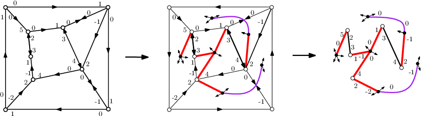
The following theorem is proved in [8]:

Theorem 3.

The mapping $\Phi$ is a bijection between the set $\widetilde{\mathcal{O}}$ of suitably $\mathbb{Z}$ -bioriented plane maps (Definition 1) and the set of $\mathbb{Z}$ -mobiles of negative excess, with the parameter-correspondence given in Figure 6.

For $M$ a suitably $\mathbb{Z}$ -bioriented plane map of outer degree $d$ , and $T=\Phi(M)$ the corresponding mobile, we call exposed the $d$ buds of the mobile $T=\Phi(M)$ created by applying the local transformation to the outer edges of $M$ (which have preliminarily been returned). The following additional claim, proved in [8], will be useful for counting purposes.

Claim 4.

Let $M$ be a suitably $\mathbb{Z}$ -bioriented plane map of outer degree $d$ , and let $T=\Phi(M)$ be the corresponding mobile. There is a bijection between the set $\vec{M}$ of all distinct corner-rooted maps obtained from $M$ by marking an outer corner (note that the cardinality of $\vec{M}$ can be less than $d$ due to symmetries), and the set $\vec{T}$ of all distinct mobiles obtained from $T$ by marking one of the $d$ exposed buds. Moreover, there is a bijection between the set $T_{\to}$ of mobiles obtained from $T$ by marking a non-exposed bud, and the set $T_{\to\circ}$ of mobiles obtained from $T$ by marking a half-edge incident to a white vertex.

Before we close this section we recall from [8] how to recover the map starting from a mobile (this description will be useful in Section 7 to compare our bijection with other known bijections). Let $T$ be a mobile (weighted or not) with negative excess $\delta$ . The corresponding fully blossoming mobile $T^{\prime}$ is obtained from $T$ by first inserting a fake black vertex in the middle of each white-white edge, and then by inserting a dangling half-edge called stem in each corner preceding a black-white edge $e$ in clockwise order around the black extremity of $e$ . A fully blossoming mobile is represented in solid lines in Figure 7 (buds and stems are respectively indicated by outgoing and ingoing arrows). Turning in counterclockwise direction around the mobile $T^{\prime}$ , one sees a sequence of buds and stems. The partial closure of $T^{\prime}$ is obtained by drawing an edge from each bud to the next available stem in counterclockwise order around $T^{\prime}$ (these edges can be drawn without crossings). This leaves $|\delta|$ buds unmatched (since the excess $\delta$ is equal to the number of stems minus the number of buds). The complete closure $\Psi(T)$ of $T$ is the vertex-rooted bioriented map obtained from the partial closure by first creating a root-vertex $v_{0}$ in the face containing the unmatched buds and joining it to all the unmatched buds, and then deleting all the white-white and black-white edges of the mobile $T$ and erasing the fake black vertices (these were at the middle of some edges); see Figure 7.

Proposition 5 ([8]).

Let $M$ be suitably $\mathbb{Z}$ -bioriented plane map, let $T=\Phi(M)$ be the associated mobile, and let $N=\Psi(T)$ be its complete closure. Then the plane map underlying $M$ is dual to the vertex-rooted map underlying $N$ .

4. Bijections for maps with one root-face

In this section, we present our bijections for plane maps. For each positive integer $d$ , we consider the class $\mathcal{C}_{d}$ of plane maps of outer degree $d$ and girth $d$ . We define some $\mathbb{Z}$ -biorientations that characterize the maps in $\mathcal{C}_{d}$ . This allows us to identify the class $\mathcal{C}_{d}$ with a subset of $\widetilde{\mathcal{O}}$ . We then specialize the master bijection to this subset of $\widetilde{\mathcal{O}}$ and obtain a bijection for maps in $\mathcal{C}_{d}$ with control on the number of inner faces in each degree $i\geq d$ . For the sake of clarity we start with the bipartite case, where the orientations and bijections are simpler.

4.1. Bipartite case

In this section, $b$ is a fixed positive integer. We start with the definition of the $\mathbb{Z}$ -biorientations that characterize the bipartite maps in $\mathcal{C}_{2b}$ .

Definition 6.

Let $M$ be a bipartite plane map of outer degree $2b$ having no face of degree less than $2b$ . A $b/(b\!-\!1)$ -orientation of $M$ is an admissible $\mathbb{Z}$ -biorientation such that every outgoing half-edge has weight 0 or -1 and

(i)

each inner edge has weight $b-1$ ,
(ii)

each inner vertex has weight $b$ ,
(iii)

each inner face $f$ has degree and weight satisfying $\deg(f)/2+w(f)=b$ .

Figure 9 shows some $b/(b\!-\!1)$ -orientations for $b=2$ and $b=3$ . Observe that for $b\geq 2$ , a $b/(b\!-\!1)$ -orientation has no 0-way edges, while for $b\leq 2$ it has no 2-way edges. Definition 6 of $b/(b\!-\!1)$ -orientations actually generalizes the one given in [8] for $2b$ -angulations. Note that $b/(b\!-\!1)$ -orientations of $2b$ -angulations are in fact $\mathbb{N}$ -biorientations since Condition (iii) implies that the weight of every outgoing half-edge is 0.

Theorem 7.

Let $M$ be a bipartite plane map of outer degree $2b$ having no face of degree less than $2b$ . Then $M$ admits a $b/(b\!-\!1)$ -orientation if and only if $M$ has girth $2b$ . In this case, there exists a unique suitable $b/(b\!-\!1)$ -orientation of $M$ .

The proof of Theorem 7 (which extends a result given in [8] for $2b$ -angulations) is delayed to Section 8. We now define the class of $\mathbb{Z}$ -mobiles that we will show to be in bijection with bipartite maps in $\mathcal{C}_{2b}$ .

Definition 8.

A $b$ -dibranching mobile is a $\mathbb{Z}$ -mobile such that half-edges incident to black vertices have weight 0 or $-1$ and

(i)

each edge has weight $b-1$ ,
(ii)

each white vertex has weight $b$ ,
(iii)

each black vertex $v$ has degree and weight satisfying $\deg(v)/2+w(v)=b$ ; equivalently a black vertex of degree $2i$ is adjacent to $i-b$ white leaves.

The two ways of phrasing Condition (iii) are equivalent because a half-edge incident to a black vertex has weight -1 if and only if it belongs to an edge incident to a white leaf. Examples of $b$ -dibranching mobiles are given in Figure 9. The possible edges of a $b$ -dibranching mobile are represented for different values of $b$ in Figure 8.

Claim 9.

Any $b$ -dibranching mobile has excess $-2b$ .

Proof.

Let $T$ be a $b$ -dibranching mobile. Let e be the number of edges and $\beta$ be the number of buds. Let $v_{b}$ and $v_{w}$ be the number of black and white vertices respectively. Let $h_{b}$ and $h_{w}$ be the number of non-bud half-edges incident to black and white vertices, respectively. By definition, the excess $\delta$ of the mobile is $\delta=h_{w}-\beta$ . Now, by Condition (iii) on black vertices, one gets $(h_{b}+\beta)/2+S=b\,v_{b}$ , where $S$ is the sum of weights of the half-edges incident to black vertices. By Conditions (i) and (ii), one gets $\textrm{e}(b-1)=b\,v_{w}+S$ . Eliminating $S$ between these relations gives $2\textrm{e}(b-1)+h_{b}+\beta=2b(v_{b}+v_{w})$ . Lastly, plugging $v_{b}+v_{w}=\textrm{e}+1$ and $2\textrm{e}=h_{b}+h_{w}$ in this relation, one obtains $h_{w}-\beta=-2b$ . ∎

We now come to the main result of this subsection, which is the correspondence between the set $\mathcal{C}_{2b}$ of bipartite maps and the $b$ -dibranching mobiles. First of all, Theorem 7 allows one to identify the set $\mathcal{C}_{2b}$ of bipartite maps with the set of $b/(b\!-\!1)$ -oriented plane maps in $\widetilde{\mathcal{O}}$ . We now consider the image of this subset of $\widetilde{\mathcal{O}}$ by the master bijection $\Phi$ . In view of the parameter-correspondence induced by the master bijection $\Phi$ (Theorem 3), it is clear that Conditions (i), (ii), (iii) of the $b/(b\!-\!1)$ -orientations correspond respectively to Conditions (i), (ii), (iii) of the $b$ -dibranching mobiles. Thus, by Theorem 3, the master bijection $\Phi$ induces a bijection between the set of $b/(b\!-\!1)$ -oriented plane maps in $\widetilde{\mathcal{O}}$ and the set of $b$ -dibranching mobiles of excess $-2b$ . Moreover, by Claim 9 the constraint on the excess is redundant. We conclude:

Theorem 10.

For any positive integer $b$ , bipartite plane maps of girth $2b$ and outer degree $2b$ are in bijection with $b$ -dibranching mobiles. Moreover, each inner face of degree $2i$ in the map corresponds to a black vertex of degree $2i$ in the mobile.

Figure 9 illustrates the bijection on two examples ( $b=2$ , $b=3$ ). The case $b=1$ and its relation with [26] is examined in more details in Section 7.

4.2. General case

We now treat the case of general (not necessarily bipartite) maps. In this subsection, $d$ is a fixed positive integer.

Definition 11.

Let $M$ be a plane map of outer degree $d$ having no face of degree less than $d$ . A $d/(d\!-\!2)$ -orientation of $M$ is an admissible $\mathbb{Z}$ -biorientation such that every outgoing half-edge has weight 0, $-1$ or $-2$ and

(i)

each inner edge has weight $d-2$ ,
(ii)

each inner vertex has weight $d$ ,
(iii)

each inner face $f$ has degree and weight satisfying $\deg(f)+w(f)=d$ .

Figure 9 shows some $d/(d\!-\!2)$ -orientations for $d=3$ and $d=5$ . The cases $d=1$ and $d=2$ are represented in Figures 15 and 13 respectively. Definition 11 of $d/(d\!-\!2)$ -orientations actually generalizes the one given in [8] for $d$ -angulations. Note that $d/(d\!-\!2)$ -orientations of $d$ -angulations are in fact $\mathbb{N}$ -biorientations since Condition (iii) implies that the weight of every outgoing half-edge is 0.

Theorem 12.

Let $M$ be a plane map of outer degree $d$ having no face of degree less than $d$ . Then, $M$ admits a $d/(d\!-\!2)$ -orientation if and only if $M$ has girth $d$ . In this case, there exists a unique suitable $d/(d\!-\!2)$ -orientation of $M$ .

Remark 13. If $d=2b$ and $M$ is a bipartite plane map of outer degree $d$ and girth $d$ , then the unique suitable $d/(d\!-\!2)$ -orientation of $M$ is obtained from its suitable $b/(b\!-\!1)$ -orientation by doubling the weight of every inner half-edge (since the $\mathbb{Z}$ -biorientation obtained in this way is clearly a suitable $d/(d\!-\!2)$ -orientation).

The proof of Theorem 12 is delayed to Section 8. We now define the class of mobiles that we will show to be in bijection with $\mathcal{C}_{d}$ .

Definition 14.

For a positive integer $d$ , a $d$ -branching mobile is a $\mathbb{Z}$ -mobile such that half-edges incident to black vertices have weight 0, $-1$ or $-2$ and

(i)

each edge has weight $d-2$ ,
(ii)

each white vertex has weight $d$ ,
(iii)

each black vertex $v$ has degree and weight satisfying $\deg(v)+w(v)=d$ .

The possible edges of a $d$ -branching mobile are represented for different values of $d$ in Figure 10. The following claim can be proved by an argument similar to the one used in Claim 9.

Claim 15.

Any $d$ -branching mobile has excess $-d$ .

We now come to the main result of this subsection, which is the correspondence between the set $\mathcal{C}_{d}$ of plane maps of girth $d$ and outer degree $d$ and the set of $d$ -branching mobiles. By Theorem 12, the set $\mathcal{C}_{d}$ can be identified with the subset of $d/(d\!-\!2)$ -oriented plane maps in $\widetilde{\mathcal{O}}$ . Moreover, as in the bipartite case, it is easy to see from Theorem 3 that the master bijection $\Phi$ induces a bijection between the set of $d/(d\!-\!2)$ -oriented plane maps in $\widetilde{\mathcal{O}}$ and the set of $d$ -branching mobiles. We conclude:

Theorem 16.

For any positive integer $d$ , plane maps of girth $d$ and outer degree $d$ are in bijection with $d$ -branching mobiles. Moreover, each inner face of degree $i$ in the map corresponds to a black vertex of degree $i$ in the mobile.

Figure 11 illustrates the bijection on two examples ( $d=3$ , $d=5$ ). The bijection of Theorem 16 is actually a generalization of the bijection given in [8] for $d$ -angulations of girth $d\geq 3$ (for $d$ -angulations there are no negative weights). The cases $d=1$ and $d=2$ of Theorem 16 are examined in more details in Section 7, in particular the relation between our bijection in the case $d=1$ and the bijection described by Bouttier, Di Francesco and Guitter in [12] (we also show a link with another bijection described by the same authors in [13]).

Remark 17. For $d=2b$ it is clear from Remark 4.2 that the bijection of Theorem 10 is equal to the specialization of the bijection of Theorem 16 to bipartite maps, up to dividing the weights of the mobiles by two.

5. Bijections for maps with two root-faces

In this section we describe bijections for annular maps. An annular map is of type $(p,q)$ if the outer and inner root-faces have degrees $p$ and $q$ respectively. We denote by $\mathcal{A}_{d}^{(p,q)}$ the class of annular maps of type $(p,q)$ with non-separating girth at least $d$ and separating girth $p$ (in particular $\mathcal{A}_{d}^{(p,q)}=\emptyset$ unless $q\geq p$ ). In the following we obtain a bijection between $\mathcal{A}_{d}^{(p,q)}$ and a class of mobiles. Our strategy parallels the one of the previous section, and we start again with the bipartite case which is simpler. In Section 6.2 we will show that counting results for the classes $\mathcal{A}_{d}^{(p,q)}$ can be used to enumerate also the annular maps with separating girth smaller than the outer degree.

5.1. Bipartite case

In this subsection we fix positive integers $b,r,s$ with $r\leq s$ . We start with the definition of the $\mathbb{Z}$ -biorientations that characterize the bipartite maps in $\mathcal{A}_{2b}^{(2r,2s)}$ .

Definition 18.

Let $M$ be a bipartite annular map of type $(2r,2s)$ having no face of degree less than $2b$ . A $b/(b\!-\!1)$ -orientation of $M$ is an admissible $\mathbb{Z}$ -biorientation such that every outgoing half-edge has weight 0 or -1 and

(i)

each inner edge has weight $b-1$ ,
(ii)

each inner vertex has weight $b$ ,
(iii)

each non-root face $f$ has degree and weight satisfying $\deg(f)/2+w(f)=b$ ,
(iv)

the inner root-face has degree $2s$ and weight $r-s$ .

Figure 12 (top left) shows a $b/(b\!-\!1)$ -orientation for $b=2$ . Note that when $r=b$ (outer root-face of degree $2b$ ) every inner face (including the inner root-face) satisfies $\deg(f)/2+w(f)=b$ , in which case we recover the definition of $b/(b\!-\!1)$ -orientations for plane bipartite maps of outer degree $2b$ , as given in Section 4.

Theorem 19.

Let $M$ be an annular bipartite map of type $(2r,2s)$ . Then $M$ admits a $b/(b\!-\!1)$ -orientation if and only if $M$ is in $\mathcal{A}_{2b}^{(2r,2s)}$ . In this case, there exists a unique suitable $b/(b\!-\!1)$ -orientation of $M$ .

The proof of Theorem 19 (which extends Theorem 7, corresponding to the case $r=b$ ) is delayed to Section 8. We now define the class of $\mathbb{Z}$ -mobiles that we will show to be in bijection with bipartite maps in $\mathcal{A}_{2b}^{(2r,2s)}$ .

Definition 20.

A $b$ -dibranching mobile of type $(2r,2s)$ is a $\mathbb{Z}$ -mobile with a marked black vertex called special vertex such that half-edges incident to black vertices have weight 0 or $-1$ and

(i)

each edge has weight $b-1$ ,
(ii)

each white vertex has weight $b$ ,
(iii)

each non-special black vertex $v$ has degree and weight satisfying $\deg(v)/2+w(v)=b$ ; equivalently a non-special black vertex of degree $2i$ is adjacent to $i-b$ white leaves.
(iv)

the special vertex $v_{0}$ has degree $2s$ and weight $r-s$ ; equivalently $v_{0}$ has degree $2s$ and is adjacent to $s-r$ white leaves.

A $2$ -dibranching mobile of type $(6,8)$ is represented in Figure 12 (bottom left). As a straightforward extension of Claim 9 we obtain:

Claim 21.

Any $b$ -dibranching mobile of type $(2r,2s)$ has excess $-2r$ .

We now come to the main result of this subsection, which is the correspondence between the set $\mathcal{A}_{2b}^{(2r,2s)}$ of annular bipartite maps and $b$ -dibranching mobiles of type $(2r,2s)$ . First of all, by Theorem 19 the set $\mathcal{A}_{2b}^{(2r,2s)}$ can be identified with the subset of $b/(b\!-\!1)$ -oriented annular maps of type $(2r,2s)$ in $\widetilde{\mathcal{O}}$ . Thus, it remains to show that the master bijection induces a bijection between this subset and the set of $b$ -dibranching mobiles of type $(2r,2s)$ . In view of the parameter-correspondence of the master bijection $\Phi$ (Theorem 3), it is clear that Conditions (i), (ii), (iii), (iv) of the $b/(b\!-\!1)$ -orientations correspond respectively to Conditions (i), (ii), (iii), (iv) of the $b$ -dibranching mobiles. Thus, by Theorem 3, the master bijection $\Phi$ induces a bijection between the set of $b/(b\!-\!1)$ -oriented annular maps of type $(2r,2s)$ in $\widetilde{\mathcal{O}}$ and the set of $b$ -dibranching mobiles of type $(2r,2s)$ and excess $-2r$ . Moreover, by Claim 21 the constraint on the excess is redundant. We conclude:

Theorem 22.

Bipartite annular maps in $\mathcal{A}_{2b}^{(2r,2s)}$ are in bijection with $b$ -dibranching mobiles of type $(2r,2s)$ . Moreover, each non-root face of degree $2i$ in the map corresponds to a non-special black vertex of degree $2i$ in the mobile.

Theorem 22 is illustrated in Figure 12 (left). Observe that the case $b=r$ in Theorem 22 corresponds to the bijection of Theorem 10 where an inner face is marked.

5.2. General case

We now treat the case of general (not necessarily bipartite) maps. In this subsection we fix positive integers $d,p,q$ with $p\leq q$ .

Definition 23.

Let $M$ be an annular map of type $(p,q)$ having no face of degree less than $d$ . A $d/(d\!-\!2)$ -orientation of $M$ is an admissible $\mathbb{Z}$ -biorientation such that every outgoing half-edge has weight 0, $-1$ or $-2$ and

(i)

each inner edge has weight $d-2$ ,
(ii)

each inner vertex has weight $d$ ,
(iii)

each non-root face $f$ has degree and weight satisfying $\deg(f)+w(f)=d$ ,
(iv)

the inner root-face has degree $q$ and weight $p-q$ .

Figure 12 (top right) shows a $d/(d\!-\!2)$ -orientation for $d=3$ . Note that when $p=d$ every inner face satisfies $\deg(f)+w(f)=d$ , in which case we recover the definition of $d/(d\!-\!2)$ -orientations for plane maps of outer degree $d$ , as given in Section 4.

Theorem 24.

Let $M$ be an annular map of type $(p,q)$ having no face of degree less than $d$ . Then, $M$ admits a $d/(d\!-\!2)$ -orientation if and only if $M$ is in $\mathcal{A}_{d}^{(p,q)}$ . In this case, there exists a unique suitable $d/(d\!-\!2)$ -orientation of $M$ .

Remark 25. If $d=2b$ and $M$ is a bipartite annular map in $\mathcal{A}_{d}^{(p,q)}$ , then the unique suitable $d/(d\!-\!2)$ -orientation of $M$ is obtained from its suitable $b/(b\!-\!1)$ -orientation by doubling the weight of every inner half-edge.

The proof of Theorem 24 (which extends Theorem 12) is delayed to Section 8.

Definition 26.

A $d$ -branching mobile of type $(p,q)$ is a $\mathbb{Z}$ -mobile with a marked black vertex called special vertex such that half-edges incident to black vertices have weight 0, $-1$ or $-2$ and

(i)

each edge has weight $d-2$ ,
(ii)

each white vertex has weight $d$ ,
(iii)

each non-special black vertex $v$ has degree and weight satisfying $\deg(v)+w(v)=d$ ,
(iv)

the special vertex has degree $q$ and weight $p-q$ .

The proof of the following claim is similar to the one used for Claim 9.

Claim 27.

Any $d$ -branching mobile of type $(p,q)$ has excess $-p$ .

We now come to the main result of this subsection, which is the correspondence between the set $\mathcal{A}_{d}^{(p,q)}$ of annular maps and $d$ -branching mobiles of type $(p,q)$ . First of all, by Theorem 24, the set $\mathcal{A}_{d}^{(p,q)}$ can be identified with the set of $d/(d\!-\!2)$ -oriented annular maps of type $(p,q)$ in $\widetilde{\mathcal{O}}$ . Moreover, as in the bipartite case, it is easy to see from Theorem 3 that the master bijection $\Phi$ induces a bijection between this subset of $\widetilde{\mathcal{O}}$ and the set of $d$ -branching mobiles of type $(p,q)$ . We conclude:

Theorem 28.

Annular maps in $\mathcal{A}_{d}^{(p,q)}$ are in bijection with $d$ -branching mobiles of type $(p,q)$ . Moreover, each non-root face of degree $i$ in the map corresponds to a non-special black vertex of degree $i$ in the mobile.

Theorem 28 is illustrated in Figure 12 (right). The case $d=p$ in Theorem 28 corresponds to the bijection of Theorem 16 where an inner face is marked.

Remark 29. For $d=2b$ it is clear from Remark 5.2 that the bijection of Theorem 22 is equal to the specialization of the bijection of Theorem 28, up to dividing the weights of the mobiles by two.

6. Counting results

In this section we derive the enumerative consequences of the bijections described in the previous sections.

6.1. Counting maps with one root-face

In this subsection we give, for each positive integer $d$ , a system of equations specifying the generating function $F_{d}$ of rooted maps of girth $d$ and outer degree $d$ counted according to the number of inner face of each degree.

We first set some notation. For any integers $p,q$ we denote by $[p\,..\,q]$ the set of integers $\{k\in\mathbb{Z},~p\leq k\leq q\}$ . If $G(x)$ is a (Laurent) formal power series in $x$ , we denote by $[x^{k}]G(x)$ , the coefficient of $x^{k}$ in $G(x)$ . For each non-negative integer $j$ we define the polynomial $h_{j}$ in the variables $w_{1},w_{2},\ldots$ by:

(1)

h_{j}(w_{1},w_{2},\ldots):=[t^{j}]\frac{1}{1-\sum_{i>0}t^{i}w_{i}}=\sum_{r\geq 0}\sum_{\begin{subarray}{c}i_{1},\ldots,i_{r}>0\\ i_{1}+\cdots+i_{r}=j\end{subarray}}w_{i_{1}}\cdots w_{i_{r}}.

In other words, $h_{j}$ is the (polynomial) generating function of integer compositions of $j$ where the variable $w_{i}$ marks the number of parts of size $i$ . Note that $h_{0}=1$ .

Let $d$ be a positive integer. By Theorem 10 and Claim 4, counting rooted plane maps of girth $d$ and outer degree $d$ reduces to counting $d$ -branching mobiles rooted at an exposed bud. To carry out the latter task we simply write the generating function equation corresponding to the recursive decomposition of trees. We call planted $d$ -branching mobile a mobile with a dangling half-edge that can be obtained as one of the two connected components after cutting a $d$ -branching mobile $M$ at the middle of an edge. The weight of the dangling half-edge $h$ is called the root-weight, and the vertex incident to $h$ is called the root-vertex. Recall that the half-edges of a $d$ -branching mobiles have weight in $[-2\,..\,d]$ . For $j$ in $[-2\,..\,d]$ , we denote by $\mathcal{W}_{j}$ the family of planted $d$ -branching mobiles of root-weight $d-2-j$ . We denote by $W_{j}\equiv W_{j}(x_{d},x_{d+1},x_{d+2}\ldots)$ the generating function of $\mathcal{W}_{j}$ , where for $k\geq d$ the variable $x_{k}$ marks the black vertices of degree $k$ . We now consider the recursive decomposition of planted mobiles and translate it into a system of equations characterizing the series $W_{-2},\ldots,W_{d}$ .

Let $j$ be in $[-2\,..\,d-3]$ , and let $T$ be a planted mobile in $\mathcal{W}_{j}$ . Since $d-2-j>0$ , the root-vertex $v$ of $T$ is white, hence is incident to half-edges having positive weights. Let $e_{1},\ldots,e_{r}$ be the edges incident to $v$ . For all $i=1\ldots r$ , let $T_{i}$ be the planted mobile obtained by cutting the edge $e_{i}$ in the middle ( $T_{i}$ is the subtree not containing $v$ ), and let $\alpha(i)>0$ be the weight of the half-edge of $e_{i}$ incident to $v$ (so that $T_{i}$ is in $\mathcal{W}_{\alpha(i)}$ ). Since the white vertex $v$ has weight $d$ , one gets the constraint $\sum_{i}\alpha(i)=j+2$ . Conversely, any sequence of planted mobiles $T_{1},\ldots,T_{r}$ in $\mathcal{W}_{\alpha(1)},\ldots,\mathcal{W}_{\alpha(r)}$ such that $\alpha(i)>0$ and $\sum_{i}\alpha(i)=j+2$ gives a planted mobile in $\mathcal{W}_{j}$ . Thus for all $j$ in $[-2\,..\,d-3]$ ,

W_{j}=\sum_{r\geq 0}\sum_{\begin{subarray}{c}i_{1},\ldots,i_{r}>0\\ i_{1}+\cdots+i_{r}=j+2\end{subarray}}W_{i_{1}}\cdots W_{i_{r}}=h_{j+2}(W_{1},\ldots,W_{d-1}).

Note that the special case $W_{-2}=1$ is consistent with our convention $h_{0}=1$ . Observe also that $W_{-1}=h_{1}(W_{1})=W_{1}$ whenever $d>1$ .

Now let $j$ be in $[d-2\,..\,d]$ , let $T$ be a planted mobile in $\mathcal{W}_{j}$ . Since $d-2-j\leq 0$ , the root-vertex $v$ of $T$ is black. If $v$ has degree $i$ , then there is a sequence of $i-1$ buds and non-dangling half-edges incident to $v$ . Each non-dangling half-edge $h$ has weight $\alpha\in\{0,-1,-2\}$ , and cutting the edge containing $h$ gives a planted mobile in $\mathcal{W}_{\alpha}$ . Lastly, Condition (iii) of $d$ -branching mobiles implies that the sum of weights of non-dangling half-edges is $d-\mathrm{deg}(v)-(d-2-j)=j+2-i$ . Conversely, any sequence of buds and non-dangling half-edges satisfying these conditions gives a planted mobile in $\mathcal{W}_{j}$ . Thus for all $j$ in $[d-2\,..\,d]$ ,

W_{j}=[u^{j+2}]\sum_{i\geq d}x_{i}u^{i}(1+W_{0}+u^{-1}W_{-1}+u^{-2})^{i-1},

where the summands $1$ , $W_{0}$ , $u^{-1}W_{-1}$ and $u^{-2}=u^{-2}W_{-2}$ in the parenthesis correspond respectively to the buds and non-dangling half-edges of weight 0, $-1$ , $-2$ incident to $v$ . We summarize:

Theorem 30.

Let $d$ be a positive integer, and let $F_{d}\equiv F_{d}(x_{d},x_{d+1},x_{d+2},\ldots)$ be the generating function of rooted maps of girth $d$ with outer degree $d$ , where each variable $x_{i}$ counts the inner faces of degree $i$ . Then,

(2)

F_{d}=W_{d-2}-\sum_{j=-2}^{d-3}W_{j}W_{d-2-j},

where $W_{-2}=1,W_{-1},W_{0},\ldots,W_{d}$ are the unique formal power series satisfying:

(3)

\left\{\begin{array}[]{ll}\displaystyle W_{j}=h_{j+2}(W_{1},\ldots,W_{d-1})&\textrm{for all }j\textrm{ in }[-2\,..\,d-3],\\[2.84544pt] \displaystyle W_{j}=[u^{j+2}]\sum_{i\geq d}x_{i}u^{i}(1+W_{0}+u^{-1}W_{-1}+u^{-2})^{i-1}&\textrm{for all }j\textrm{ in }[d-2\,..\,d],\\ \end{array}\right.

where the polynomials $h_{j}$ are defined by (1). In particular, for any finite set $\Delta\subset\{d,d+1,d+2,\ldots\}$ , the specialization of $F_{d}$ obtained by setting $x_{i}=0$ for all $i$ not in $\Delta$ is algebraic (over the field of rational function in $x_{i},i\in\Delta$ ).

For $d=1$ , Theorem 30 gives exactly the system of equations obtained by Bouttier, Di Francesco and Guitter in [12]. Observe that for any integer $d\geq 2$ the series $W_{-1}$ and $W_{1}$ are equal, so the number of unknown series is $d+1$ in these cases. Moreover for $d\geq 1$ the series $W_{d}$ is not needed to define the other series $W_{0},W_{1},\ldots,W_{d-1}$ . Lastly, under the specialization $\{x_{d}=x,\ x_{i}=0\ \forall i>d\}$ one gets $W_{d-1}=W_{d}=0$ and $W_{d-2}=x(1+W_{0})^{d-1}$ ; in this case we recover the system of equations given in [8] for the generating function of rooted $d$ -angulations of girth $d$ .

Proof.

The fact that the solution of the system (3) is unique is clear. Indeed, it is easy to see that the series $W_{-1},W_{0},\ldots,W_{d}$ have no constant terms, and from this it follows that the coefficients of these series are uniquely determined by induction on the total degree.
We now prove (2). By Theorem 16 and Claim 4 (first assertion) the series $F_{d}$ is equal to the generating function of $d$ -branching mobiles with a marked exposed bud (where $x_{k}$ marks the black vertices of degree $k$ ). Moreover by the second assertion of Claim 4, $F_{d}$ is equal to the difference between the generating function $B_{d}$ of $d$ -branching mobiles with a marked bud, and the generating function $H_{d}$ of $d$ -branching mobiles with a marked half-edge incident to a white vertex. Lastly, $B_{d}=W_{d-2}$ because $d$ -branching mobiles with a marked bud identify with planted mobiles in $\mathcal{W}_{d-2}$ , and $H_{d}=\sum_{j=-2}^{d-3}W_{j}W_{d-2-j}$ because $d$ -branching mobiles with a marked half-edge incident to a white vertex are in bijection (by cutting the edge) with ordered pairs $(T,T^{\prime})$ of planted $d$ -branching mobiles in $\mathcal{W}_{j}\times\mathcal{W}_{d-2-j}$ for some $j$ in $[-2\,..\,d-3]$ . ∎

We now explore the simplifications occurring in the bipartite case.

Theorem 31.

Let $b\geq 1$ , and let $E_{b}\equiv F_{2b}(x_{2b},0,x_{2b+2},0,x_{2b+4}\ldots)$ be the generating function of rooted bipartite maps of girth $2b$ with outer degree $2b$ , where each variable $x_{2i}$ marks the number of inner faces of degree $2i$ . Then,

(4)

E_{b}=V_{b-1}-\sum_{j=-1}^{b-2}V_{j}V_{b-j-1},

where $V_{-1}=1,V_{0},\ldots,V_{b}$ are the unique formal power series satisfying:

(5)

\left\{\begin{array}[]{lll}\displaystyle V_{j}=h_{j+1}(V_{1},\ldots,V_{b-1})&\textrm{for all }j\textrm{ in }[-1\,..\,b-2],\\[2.84544pt] \displaystyle V_{j}=\sum_{i\geq b}x_{2i}\binom{2i-1}{i-j-1}(1+V_{0})^{i+j}&\textrm{for all }j\textrm{ in }\{b-1,b\}.\end{array}\right.

Theorem 31 can be obtained by a direct counting of $b$ -dibranching mobiles (which are simpler than $d$ -branching mobiles). However in the proof below we derive Theorem 31 as a consequence of Theorem 30.

Proof.

Equations (4) and (5) are obtained respectively from (2) and (3) simply by setting for all integer $i$ , $x_{2i+1}=0$ , $W_{2i}=V_{i}$ , $W_{2i+1}=0$ . Hence we only need to prove that the series $W_{i}$ defined by (2) satisfy for all $i$ , $W_{2i+1}(x_{2b},0,x_{2b+2},0,\ldots)=0$ . This property holds because one can show that every monomial in the series $W_{2i+1}(x_{2b},x_{2b+1},x_{2b+2},\ldots),i\in\mathbb{Z}$ contains at least one variable $x_{r}$ with $r$ odd, by a simple induction on the total degree of these monomials. ∎

6.2. Counting maps with two root-faces

In this subsection we count rooted annular maps according to the face degrees and according to the two girth parameters. For positive integers $d,e,p,q$ , we denote by $\mathcal{A}_{d,e}^{(p,q)}$ the class of annular maps of type $(p,q)$ having non-separating girth at least $d$ and separating girth at least $e$ . Recall that an annular map is rooted if a corner is marked in each of the root-faces. We will now derive an expression for the generating functions $G_{d,e}^{(p,q)}$ of maps obtained by rooting the annular maps in $\mathcal{A}_{d,e}^{(p,q)}$ .

Theorem 32.

For any positive integers $d,e,p,q$ , the series $G_{d,e}^{(p,q)}=G_{d,e}^{(p,q)}(x_{d},x_{d+1},\ldots)$ counting rooted annular maps of type $(p,q)$ with non-separating girth at least $d$ and separating girth at least $e$ (where $x_{k}$ marks the number of non-root faces of degree $k$ ) is

(6)

G_{d,e}^{(p,q)}=\sum_{i=0}^{p-e}\sum_{j=0}^{q-e}\mathbf{1}_{i+j\equiv p+q\ (\mathrm{mod}\ 2)}\,\frac{2\beta(p,i,e)\beta(q,j,e)}{p+q-i-j}(1+W_{0})^{(p+q-i-j)/2}W_{-1}\ \!\!^{i+j},

where the formal power series $W_{-1},W_{0},\ldots,W_{d}$ are specified by (3), and where

\displaystyle\beta(p,i,e):=\frac{p!}{i!\lfloor\tfrac{p-i-e}{2}\rfloor!\lfloor\tfrac{p-i+e-1}{2}\rfloor!}.

Proof.

The proof has two parts. First we will use the bijection obtained in Section 5 in order to characterize the series $G_{d,e}^{(p,q)}$ in the case $e=p$ . Then we will treat the case of an arbitrary separating girth $e\geq p$ (in the case $e<p$ , $G_{d,e}^{(p,q)}=0$ ).

By definition the series $G_{d,p}^{(p,q)}$ counts maps obtained by rooting the annular maps in $\mathcal{A}_{d}^{(p,q)}\equiv\mathcal{A}_{d,p}^{(p,q)}$ . Let $\mathcal{X}$ be the set of $d$ -branching mobiles of type $(p,q)$ with a marked corner at the special vertex. By Theorem 28 maps in $\mathcal{A}_{d}^{(p,q)}$ are in bijection with the $d$ -branching mobiles of type $(p,q)$ . Hence it is easy to see from the definition of the master bijection $\Phi$ that maps obtained by marking a corner in the inner root-face of a map in $\mathcal{A}_{d}^{(p,q)}$ are in bijection with the mobiles in $\mathcal{X}$ . Hence, maps obtained by rooting the annular maps in $\mathcal{A}_{d}^{(p,q)}$ are in $p$ -to-1 correspondence with the mobiles in $\mathcal{X}$ . It remains to count the mobiles in $\mathcal{X}$ . Let $M$ be a mobile in $\mathcal{X}$ and let $v_{0}$ be the special vertex. The vertex $v_{0}$ is black and is incident to a sequence of $q$ buds and non-dangling half-edges. Each non-dangling half-edge $h$ incident to $v_{0}$ has a weight $\alpha$ in $\{0,-1,-2\}$ , and cutting the edge containing $h$ gives a planted mobile in $\mathcal{W}_{\alpha}$ . Moreover the total weight of the non-dangling half-edges incident to $v_{0}$ is $p-q$ . Conversely any sequence of $q$ buds and non-dangling half-edges satisfying these conditions gives a mobile in $\mathcal{X}$ . This bijective decomposition of the mobiles in $\mathcal{X}$ gives an expression for the generating function of $\mathcal{X}$ , or equivalently for the series $G_{d,p}^{(p,q)}$ :

(7)

G_{d,p}^{(p,q)}=p\cdot[u^{p-q}](1+W_{0}+u^{-1}W_{-1}+u^{-2})^{q}.

Here the summands $1$ , $W_{0}$ , $u^{-1}W_{-1}$ and $u^{-2}=u^{-2}W_{-2}$ correspond respectively to the buds and to the half-edges of weight 0, $-1$ , $-2$ incident to the special vertex.

We will now derive an expression for the series $G_{d,e}^{(p,q)}$ when $e\geq p$ . We first partition the set $\mathcal{A}_{d,e}^{(p,q)}$ . For $a\leq\mathrm{min}(p,q)$ , we denote by $\widetilde{\mathcal{A}}_{d,a}^{(p,q)}$ the class of annular maps of type $(p,q)$ having non-separating girth at least $d$ , and separating girth exactly $a$ . Let $\widetilde{G}_{d,a}^{(p,q)}\equiv\widetilde{G}_{d,a}^{(p,q)}(x_{d},x_{d+1},\ldots)$ be the generating function counting rooted annular maps from $\widetilde{\mathcal{A}}_{d,a}^{(p,q)}$ . Clearly, $\mathcal{A}_{d,e}^{(p,q)}=\uplus_{a=e}^{\min(p,q)}\widetilde{\mathcal{A}}_{d,a}^{(p,q)}$ , so that $G_{d,e}^{(p,q)}=\sum_{a=e}^{\mathrm{min}(p,q)}\widetilde{G}_{d,a}^{(p,q)}$ .

For $p\leq q$ we denote by $\widehat{\mathcal{A}}_{d}^{(p,q)}$ the subfamily of $\mathcal{A}_{d}^{(p,q)}$ where the unique separating cycle of length $p$ is the contour of the outer face, and we denote by $\widehat{G}_{d}^{(p,q)}\equiv\widehat{G}_{d}^{(p,q)}(x_{d},x_{d+1},\ldots)$ the generating function counting rooted annular maps from $\widehat{\mathcal{A}}_{d}^{(p,q)}$ . Let $M$ be a rooted annular map from $\mathcal{A}_{d}^{(p,q)}$ . It is easy to see that there exists a unique innermost cycle $C$ of length $p$ enclosing the inner root-face (i.e., any other cycle of length $p$ enclosing the inner root-face also encloses $C$ ). The cycle $C$ is simple, and after distinguishing one of the $p$ vertices on $C$ , one can identify the part of $M$ outside and inside $C$ as rooted annular maps $M_{1}$ and $M_{2}$ from $\mathcal{A}_{d}^{(p,p)}$ and $\widehat{\mathcal{A}}_{d}^{(p,q)}$ respectively (the marked vertex of $C$ gives the marked corners of the inner root-face of $M_{1}$ and the outer root-face of $M_{2}$ ). This bijective decomposition of $M$ gives $p\,G_{d,p}^{(p,q)}=G_{d,p}^{(p,p)}\cdot\widehat{G}_{d}^{(p,q)}$ , or equivalently,

\widehat{G}_{d}^{(p,q)}=p\,\frac{G_{d,p}^{(p,q)}}{G_{d,p}^{(p,p)}}.

Now, given a rooted annular map $M$ from $\widetilde{\mathcal{A}}_{d,a}^{(p,q)}$ with root-faces $f_{1}$ and $f_{2}$ , we consider the outermost and innermost cycles $C_{1}$ and $C_{2}$ of length $a$ separating $f_{1}$ from $f_{2}$ . By distinguishing some vertices $v_{1}$ and $v_{2}$ from $C_{1}$ and $C_{2}$ and cutting $M$ along $C_{1}$ and $C_{2}$ one obtains three rooted annular maps respectively from $\widehat{\mathcal{A}}_{d}^{(a,p)}$ , $\mathcal{A}_{d}^{(a,a)}$ , and $\widehat{\mathcal{A}}_{d}^{(a,q)}$ (the root-corner in the root-face enclosed by $C_{1}$ is the one incident to $v_{1}$ , and the root-corner in the root-face enclosed by $C_{2}$ is the one incident to $v_{2}$ ). This decomposition yields

a^{2}\widetilde{G}_{d,a}^{(p,q)}=\widehat{G}_{d}^{(a,p)}G_{d,a}^{(a,a)}\widehat{G}_{d}^{(a,q)}=a^{2}\frac{G_{d,a}^{(a,p)}G_{d,a}^{(a,q)}}{G_{d,a}^{(a,a)}}.

By (7),

G_{d,a}^{(a,p)}=a\sum_{i=0}^{p-a}\gamma(p,i,a)\,(1+W_{0})^{(p+a-i)/2}{W_{-1}}^{i}

where $\displaystyle\gamma(p,i,a)=\mathbf{1}_{p-i\equiv a\ (\mathrm{mod}\ 2)}\frac{p!}{i!(\tfrac{p-i-a}{2})!(\tfrac{p-i+a}{2})!}$ . Hence, for $a\leq\min(p,q)$ ,

\widetilde{G}_{d,a}^{(p,q)}=\sum_{i=0}^{p-a}\sum_{j=0}^{q-a}a\,\gamma(p,i,a)\gamma(q,j,a)\,(1+W_{0})^{(p+q-i-j)/2}{W_{-1}}^{i+j}.

To conclude we have

G_{d,e}^{(p,q)}=\sum_{i=0}^{p-e}\sum_{j=0}^{q-e}\ \sum_{a=e}^{\min(p-i,q-j)}a\,\gamma(p,i,a)\gamma(q,j,a)\,(1+W_{0})^{(p+q-i-j)/2}{W_{-1}}^{i+j}.

Moreover, the identity

\sum_{a=e}^{\min(p-i,q-j)}a\,\gamma(p,i,a)\gamma(q,j,a)=\mathbf{1}_{i+j\equiv p+q\ (\mathrm{mod}\ 2)}\cdot\frac{2\beta(p,i,e)\beta(q,j,e)}{p+q-i-j}

can be obtained by a simple induction on $e$ , decreasing from the base case $e=\min(p-i,q-j)$ . Indeed, if $e\equiv p-i\equiv q-j\,(\mathrm{mod}\ 2)$ , one has

\frac{2}{p+q-i-j}\left(\beta(p,i,e)\beta(q,j,e)-\beta(p,i,e+1)\beta(q,j,e+1)\right)=e\,\gamma(p,i,e)\gamma(q,j,e),

and $\beta(p,i,e-1)=\beta(p,i,e)$ , $\beta(q,j,e-1)=\beta(q,j,e)$ .
This completes the proof of Theorem 32. ∎

As a corollary we obtain the following universal asymptotic behavior for the number of $n$ -faces rooted maps with restrictions on the girth and face-degrees (as mentioned in the introduction, a result of a similar flavor was established by Bender and Canfield for bipartite maps [2], with no control on the girth):

Corollary 33.

For any non-empty finite set $\Delta\subset\{d,d+1,d+2,\ldots\}$ , the specialization of $G_{d,e}^{(p,q)}$ obtained by setting $x_{i}=0$ for all $i$ not in $\Delta$ is algebraic (over the field of rational function in $x_{i},i\in\Delta$ ). Moreover, there exist computable constants $\kappa,\gamma$ depending on $d$ and $\Delta$ such that if $\Delta$ contains at least one even integer (resp. $\Delta$ contains only odd integers) the number $c_{d,\Delta}(n)$ of rooted plane maps of girth at least $d$ with $n$ faces (resp. $2n$ faces), all of them having degrees in $\Delta$ , is asymptotically equivalent to $\kappa\,n^{-5/2}\,\gamma^{n}$ .

Proof.

The algebraicity of the series $W_{-2}\ldots W_{d}$ is obvious from the system (3), hence $G_{d,e}^{(p,q)}$ is algebraic (as soon as $\Delta$ is finite).

We now consider the specialization of the series $W_{-2}\ldots W_{d}$ and $G_{d,e}^{(p,q)}$ obtained by replacing all the variable $x_{i},i\in\Delta$ by $t$ (and setting the other variables $x_{i}$ to 0). We suppose first that $\Delta$ contains at least one even integer. Given the form of the system (3), the Drmota-Lalley-Wood theorem (see [19, VII.6]) implies that the series $W_{i},i\in[-1..d-1]$ all have the same “square-root type” singularity at their unique dominant singularity $\gamma$ . Therefore, the same applies to $G_{d,e}^{(p,q)}$ , implying $[t^{n}]G_{d,e}^{(p,q)}\sim\alpha\,n^{-3/2}\gamma^{n}$ for some computable constants $\alpha,\gamma$ (depending on $p,q,d,e,\Delta$ ). Observe that $\frac{1}{q}[t^{n}]G_{d,d}^{(p,q)}$ counts rooted plane maps of girth at least $d$ , with a root-face of degree $p$ , a marked inner face of degree $q$ , and $n$ additional inner faces having degrees in $\Delta$ . Therefore,

(n+1)\,c_{d,\Delta}(n+2)=\sum_{p,q\in\Delta}\frac{1}{q}[t^{n}]G_{d,d}^{(p,q)}.

This gives the claimed asymptotic form of $c_{d,\Delta}(n)$ when $\Delta$ contains an even integer.

If $\Delta$ contains only odd integers, one has to deal with the periodicity of the series $W_{i},i\in[-1..d-1]$ (one can easily check that $[t^{i}]W_{j}=0$ unless $i\equiv j\ (\mathrm{mod}\ 2)$ , and $[t^{n}]G_{d,e}^{(p,q)}=0$ unless $n\equiv p+q\ (\mathrm{mod}\ 2)$ ). However, up to using a variable $z=t^{2}$ , one can still use the Drmota-Lalley-Wood theorem to prove the asymptotic form $[t^{2n}]G_{d,e}^{(p,q)}\sim\alpha\,n^{-3/2}\,\gamma^{n}$ for $p,q\in\Delta$ , from which the stated result follows. ∎

As in Section 6.1, the generating functions have a simpler expression in the bipartite case:

Theorem 34.

For $b,c,r,s$ positive integers, let $B_{b,c}^{(r,s)}\equiv G_{2b,2c}^{(2r,2s)}(x_{2b},0,x_{2b+2},0,\ldots)$ be the generating function of rooted annular bipartite maps from $\mathcal{A}_{2b,2c}^{(2r,2s)}$ , where each variable $x_{2i}$ marks the number of inner faces of degree $2i$ . Then,

(8)

B_{b,c}^{(r,s)}=\frac{4rs}{r+s}\binom{2r-1}{r-c}\binom{2s-1}{s-c}(1+V_{0})^{r+s},

where $V_{0},\ldots,V_{b}$ are given by (5).

Proof.

Again the expression can either be obtained by a direct counting of $b$ -dibranching mobiles (which are simpler than $d$ -branching mobiles), or just by specializing the expression in Theorem 32. As we have seen in the proof of Theorem 31, when $x_{2i+1}=0$ for all integer $i$ , then $W_{r}=0$ for all odd $r\in[-1..d]$ and the series $V_{i}:=W_{2i}$ satisfy (5). Since $W_{-1}=0$ , there remains only the initial term ( $i=0$ and $j=0$ ) in the expression (6) of $G_{2b,2c}^{(2r,2s)}(x_{2b},0,x_{2b+2},0,x_{2b+4}\ldots)$ , which gives (8). ∎

6.3. Exact formula for simple bipartite maps

In this subsection, we obtain a closed formula for the number of rooted simple bipartite maps from the case $b=2$ of Theorem 34.

Proposition 35 (simple bipartite maps).

Let $k\geq 2$ , and let $n_{2},n_{3},\ldots,n_{k}$ be non-negative integers not all equal to zero. The number of rooted simple bipartite maps with $n_{i}$ faces of degree $2i$ for all $i\in\{2,3,\ldots,k\}$ is

(9)

2\frac{(e+n-3)!}{(e-1)!}\prod_{i=2}^{k}\frac{1}{n_{i}!}\binom{2i-1}{i-2}^{n_{i}},

where $n=\sum_{i}n_{i}$ is the number of faces, and $e=\sum_{i}in_{i}$ is the number of edges.

Proof.

Let $a(n_{2},\ldots,n_{k})$ be the number of rooted simple bipartite maps with $n_{i}$ faces of degree $2i$ for $i\in[2..k]$ . If $\sum_{i}n_{i}=1$ (i.e., the map has a single face), Formula (9) gives the $e$ th Catalan number, which indeed counts rooted plane trees with $e$ edges. We now suppose $\sum_{i}n_{i}\geq 2$ and consider integers $r,s$ such that $\bar{n}_{i}:=n_{i}-\mathbf{1}_{i=r}-\mathbf{1}_{i=s}$ is non-negative for all $i\in[2..k]$ . Let $N$ be the number of rooted annular maps of type $(2r,2s)$ with $\bar{n}_{i}$ non-root faces of degree $2i$ for $i\in[2..k]$ . Counting in two different ways rooted annular maps with a third root (a marked corner) placed anywhere, we obtain $2eN=4rsn_{r}n_{s}a(n_{2},\ldots,n_{k})$ if $r\neq s$ and $2eN=4rsn_{r}(n_{r}-1)a(n_{2},\ldots,n_{k})$ if $r=s$ . Thus it remains to prove

(10)

N=4rs\frac{(e+n-3)!}{e!}\prod_{i=2}^{k}\frac{1}{\bar{n}_{i}!}\binom{2i-1}{i-2}^{n_{i}}.

By Theorem 34, $N$ is the coefficient $[x_{2}^{\bar{n}_{2}}\ldots x_{k}^{\bar{n}_{k}}]$ of the series

B_{r,s}^{(2,2)}=\frac{4rs}{r+s}\binom{2r-1}{r-2}\binom{2s-1}{s-2}R^{r+s},

where the series $R\equiv 1+V_{0}$ is specified by $R=1+\sum_{i\geq 2}x_{2i}\binom{2i-1}{i-2}R^{i+1}$ . The Lagrange inversion formula yields

(11)

[x_{2}^{\bar{n}_{2}}\ldots x_{k}^{\bar{n}_{k}}]R^{a}=a\frac{(\sum_{i}(i+1)\bar{n}_{i}+a-1)!}{(\sum_{i}i\bar{n}_{i}+a)!\bar{n}_{2}!\ldots\bar{n}_{k}!}\prod_{i=2}^{k}\binom{2i-1}{i-2}^{\bar{n}_{i}},

which gives (10). ∎

Remark 36. With some little efforts, the proof above can be made bijective. Indeed it is not very hard to obtain the expression (11) of the coefficients of $R^{a}$ bijectively starting from the combinatorial description of the 2-dibranching mobiles.

6.4. Counting loopless maps

In this subsection, we focus on the case $d=2$ of Theorem 30 and show how to deduce from it the formula given in [31] (where it is obtained by a substitution approach) for the number of rooted loopless maps with $n$ edges. First observe that, up to collapsing the root-face of degree 2 into an edge, rooted maps in $\mathcal{C}_{2}$ identify with rooted loopless maps with at least one edge (without constraint on the degree of the root-face). Hence, the multivariate series $F_{2}$ counts rooted loopless maps with at least one edge, where $x_{i}$ marks the number of faces of degree $i$ . We now consider the specialization $x_{i}=t^{i}$ in $F_{2}$ , which gives the generating function of rooted loopless maps with at least one edge counted according to the number of half-edges. This series is defined by the system of equations (3) in the case $d=2$ , under the specialization $x_{i}=t^{i}$ . Using the notation $R:=1+W_{0}$ and $S:=W_{-1}=W_{1}$ , this system becomes

F_{2}(t^{2},t^{3},t^{4},\ldots)=R-1-S^{2}-t\,B_{3},\qquad R=1+t\,B_{1},\qquad S=t\,B_{2},

where $B_{k}=[u^{k}]B$ and

B=\sum_{i\geq 0}t^{i}(uR+S+u^{-1})^{i}.

Now we observe that $B_{k}$ is the series of Motzkin paths ending at height $k$ where up steps, horizontal steps, and down steps have respective weights $tR$ , $tS$ , and $t$ . The paths ending at height $0$ are called Motzkin bridges, and have generating function $B_{0}$ . The paths ending at height $0$ and having non-negative height all the way are called Motzkin excursions, and we denote by $M$ their generating function. It is a classical exercise to show the following identities:

(i)~B_{k}=B_{0}\,(tRM)^{k},~~~~(ii)~M=1+tSM+t^{2}RM^{2},~~~~(iii)~B_{0}=1+tSB_{0}+2t^{2}RMB_{0}.

In particular $(i)$ gives

(iv)~R=1+t^{2}B_{0}MR,~~~~\textrm{ and }~~~(v)~S=t^{3}B_{0}M^{2}R^{2}.

So we have a system of four equations $\{(ii),(iii),(iv),(v)\}$ for the unknown series $\{M,B_{0},R,S\}$ , and this system has clearly a unique power series solution. With the help of a computer algebra system, one can extract the first coefficients and then guess and check that the solution is $\{M=\alpha,\ B_{0}=\alpha^{2},\ R=\alpha,\ S=t^{3}\alpha^{6}\}$ , where the series $\alpha\equiv\alpha(t)$ is specified by $\alpha=1+t^{2}\alpha^{4}$ . Hence, $F_{2}(t^{2},t^{3},\ldots)=\alpha^{2}(2-\alpha)-1$ . We summarize:

Proposition 37.

Let $c_{n}$ be the number of rooted loopless maps with $n$ edges and let $C(t)=\sum_{n\geq 0}c_{n}t^{n}$ . Then, $C(t)=\alpha^{2}(2-\alpha)$ , where $\alpha\equiv\alpha(t)$ is the unique formal power series satisfying $\alpha=1+t\alpha^{4}$ . Hence, by the Lagrange inversion formula,

(12)

c_{n}=\frac{2(4n+1)!}{(n+1)!(3n+2)!}.

Formula (12) was already obtained in [31] using a substitution approach. The sequence $\tfrac{2(4n+1)!}{(n+1)!(3n+2)!}$ appears recurrently in combinatorics, for instance it also counts rooted simple triangulations with $n+3$ vertices [28, 24], and intervals in the $n$ th Tamari lattice [16, 4].

7. Special cases $b=1$ and $d=0,1,2$ .

In this section, we take a closer look at the bijections given in Section 4 in the particular cases $b=1$ and $d=1,2$ . We also explain how to include the case $d=0$ .

7.1. Case $b=1$ (general bipartite maps) and relation with [26]

Let $\mathcal{B}$ be the class of bipartite plane maps of outer degree 2. Note that maps in $\mathcal{B}$ have girth 2 (since bipartite maps cannot have cycles of length 1). Moreover, $\mathcal{B}$ can be identified with the class of bipartite maps with a marked edge (since the root-face of degree 2 can be collapsed into a marked edge). The case $b=1$ of Theorem 10 (illustrated in Figure 13) gives a bijection between the class $\mathcal{B}$ , and the class of 1-dibranching mobiles. We now take a closer look at this bijection and explain its relation with [26]. In [26] Schaeffer obtained a bijection for Eulerian maps (maps with vertices of even degree) with a marked edge. From the above remarks it follows that the class of Eulerian maps with a marked edges can be identified with the class $\mathcal{B}$ via duality.

Observe from Figure 8 that 1-dibranching mobiles have only two types of edges, and that their weights are redundant. Moreover all the white vertices are leaves. Hence, it is easy to see that the class of 1-dibranching mobiles identifies with the class of (unweighted) bicolored plane trees such that white vertices are leaves, and any black vertex adjacent to $\ell$ white leaves has degree $2+2\ell$ . These are exactly the blossoming trees defined by Schaeffer in [26] (the white leaves are called “stems” there). Moreover the bijection of Schaeffer coincides with ours via duality: to obtain the map from the tree, the closure operations described respectively in Proposition 5 and in [26] are the same.

The following formula (originally due to Tutte [29]) for the number $b[n_{1},\ldots,n_{k}]$ of rooted bipartite maps with $n_{i}$ faces of degree $2i$ for $1\leq i\leq k$ can be obtained by counting blossoming trees (i.e., 1-dibranching mobiles) as done by Schaeffer in [26]:

b[n_{1},\ldots,n_{k}]=2\frac{e!}{v!}\prod_{i=1}^{k}\frac{1}{n_{i}!}\binom{2i-1}{i-1}^{n_{i}},

where $e=\sum_{i}in_{i}$ and $v=2+e-\sum_{i}n_{i}$ .

7.2. Case $d=2$ (loopless maps) and relation with [27, Thm. 2.3.4]

We call edge-marked loopless map a loopless planar maps with a marked edge. It is clear that the class $\mathcal{C}_{2}$ (plane maps of girth $2$ and outer degree $2$ ) can be identified with the class of edge-marked loopless maps (since the root-face of degree 2 can be collapsed into a marked edge). Hence, for $d=2$ , Theorem 16 gives a bijection between edge-marked loopless maps and 2-branching mobiles. Some cases of this bijection are represented in Figure 13.

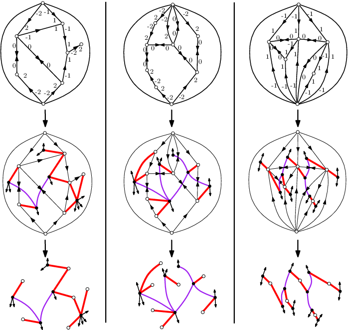
Observe from Figure 10 that 2-branching mobiles have only three types of edges, and that their weights are redundant. Up to forgetting these weights, the 2-branching mobiles are the bicolored plane trees such that there is no white-white edges, white vertices have degree 1 or 2, and black vertices adjacent to $\ell$ white leaves are incident to a total of $\ell+2$ buds or black-black edges. We now consider the specialization of our bijection for $d=2$ to triangulations (right of Figure 13), and its relation with the bijection described by Schaeffer in [27, Thm. 2.3.4] for bridgeless cubic maps (these are the dual of loopless triangulations). By the preceding remarks, Theorem 16 yields a bijection between edge-marked loopless triangulations and the mobiles with the following properties: there are no white-white edges, every white vertex has degree 2, and every black vertex has degree 3 and is adjacent to a unique white vertex. Clearly, these mobiles identify with the (unicolored) binary trees endowed with a perfect matching of the inner nodes. These are exactly the blossoming trees shown to be in bijection with bridgeless cubic maps in [27, Thm. 2.3.4] (see also [23]). Moreover, the bijection in [27, Thm. 2.3.4] coincides with ours via duality: to obtain the map from the tree, the closure operations described respectively in Proposition 5 and in [27, Thm. 2.3.4] are the same.

7.3. Case $d=1$ (general maps) and relation with [12].

The case $d=1$ of Theorem 16 gives a bijection between the class $\mathcal{C}_{1}$ and 1-branching mobiles. By definition, $\mathcal{C}_{1}$ is the class of plane maps of girth $1$ and outer degree $1$ . Hence, $\mathcal{C}_{1}$ is the class of plane maps without girth constraint such that the root-face is a loop. Note that this class can be identified with the class of rooted planar maps (indeed the root-face can be collapsed and thought as simply marking a corner). We now take a closer look at the bijection between the class $\mathcal{C}_{1}$ and 1-branching mobiles, and its relation with [12]. In [12] Bouttier, Di Francesco and Guitter obtained a bijection for $1$ -legged maps, that is, planar maps with a marked vertex of degree $1$ . Observe that the class of $1$ -legged maps identifies with the class $\mathcal{C}_{1}$ by duality (the marked vertex of degree 1 becomes a marked face of degree 1 via duality).

We will first characterize the suitable $1/(-1)$ -orientations. Let $M$ be a rooted map. We call root-distance of a vertex $v$ the minimal length of the paths joining the root-vertex and $v$ . A spanning tree of $M$ is a BFS-tree (or bread-first-search tree) if the root-distance of any vertex is the same in the map and in the tree. The root-distances and a BFS-tree are shown in Figure 14. Let $T$ be a BFS-tree and let $e$ be an edge not in $T$ . The edge $e$ creates a cycle with $T$ which separates two regions of the plane. We call left-to-right orientation of $e$ the orientation such that the region on the left of $e$ contains the root-face. The outgoing and ingoing half-edges of $e$ are then called left and right half-edges. It is easy to see (see e.g. [5]) that there exists a unique BFS-tree, called rightmost BFS-tree, such that the root-distance does not decrease along edges not in $T$ traversed left-to-right. The following characterization of suitable $1/(-1)$ -orientations is illustrated in Figure 14.

Proposition 38.

Let $M$ be a map in $\mathcal{C}_{1}$ and let $T$ be its rightmost BFS-tree. Then, the suitable $1/(-1)$ -orientation of $M$ is obtained as follows:

•

Every edge in $T$ is 1-way, oriented from parent to child with weight $-2$ on the outgoing half-edge and weight 1 on the ingoing half-edge.
•

Every inner edge $e$ not in $T$ is 0-way with weight 0 and $-1$ on the half-edges. The weight $0$ is given to the left half-edge if the root-distance of the two endpoints of $e$ is the same and to the right half-edge otherwise.

We omit the (easy but tedious) proof of Proposition 38. We now examine 1-branching mobiles and their relation with the well-charged trees considered in [12]. A charged tree is a plane tree with two types of dangling half-edges called white arrows and black arrows. The charge of a subtree $T^{\prime}$ is the number of white arrows minus the number of black arrows in $T^{\prime}$ . A well-charged tree is a charged tree such that cutting any edge gives two subtrees of charge 0 and -1 respectively. Now, observe from Figure 10 that there are only two types of edges in 1-branching mobiles: black-white with weights $(-2,1)$ or black-black with weights $(0,-1)$ . It is easily seen that 1-branching mobiles are the mobile with these two type of edges such that white vertices are leaves and each black vertex $v$ has degree and weight satisfying $\deg(v)+w(v)=1$ . For a 1-branching mobile $B$ , we denote by $\gamma(B)$ the charged tree obtained by replacing white leaves and buds respectively by white arrows and black arrows. The mapping $\gamma$ is represented in Figure 15. It is easy to check that for any black-black edge $e$ of $B$ , the charges of the subtrees obtained by deleting the edge $e$ from $\gamma(B)$ are equal to the weights of the half-edges of $e$ incident to these subtrees. From this observation it easily follows that $\gamma$ is a bijection between 1-branching mobiles and well-charged trees.

In [12] a bijection was described between $1$ -legged maps and well-charged trees. This bijection actually coincide with ours via duality (and the identification $\gamma$ between 1-branching mobiles and well-charged trees). Indeed to obtain the map from the tree, the closure operations, described respectively in Proposition 5 and in [12], are the same (and the opening operations, to get the tree from the map, rely in the same way on the rightmost BFS tree).

7.4. The case $d=0$ and relation with [13].

We show here that a slight reformulation of our bijections allows us to include the case $d=0$ , thereby recovering a bijection obtained by Bouttier, Di Francesco and Guitter in [13].

We call plane maps of outer degree 0 a planar map with a marked vertex called outer vertex. Any face, any edge and any non-marked vertex of such a map is called inner. A biorientation of a plane map of outer degree 0 is called accessible if every inner vertex can be reached from the outer vertex, it is called minimal if every directed simple cycle has the outer vertex strictly on its left, and it is called admissible if every half-edge incident to the outer vertex is outgoing. We then say that a biorientation of a plane map of outer degree 0 is suitable if it is minimal, admissible and accessible. We now reformulate the definition of $d/(d\!-\!2)$ -orientations so as to include the case $d=0$ : these are the admissible biorientations of plane maps of outer degree $d$ with inner and outer half-edges having weights in $d\cup\{1,2,3\ldots\}$ and $\{-2,-1,0\}\backslash\{d\}$ respectively, and satisfying the conditions (i),(ii),(iii) of Definition 11 (hence the definition is unchanged for $d>0$ ).

For a plane map of outer degree 0, we consider the root-distance $D(v)$ of each vertex $v$ (its graph distance to the outer vertex) and the geodesic biorientation, that is, the biorientation where an edge $\{v,v^{\prime}\}$ with $D(v^{\prime})=D(v)$ is oriented $0$ -way with weight $-1$ on each half-edge, while an edge $\{v,v^{\prime}\}$ with $D(v^{\prime})=D(v)+1$ is oriented $1$ -way toward $v^{\prime}$ with weight $-2$ on the outgoing half-edge and 0 on the ingoing half-edge.

Proposition 39.

Theorem 12 holds for all $d\geq 0$ : a plane map of outer degree $d$ admits a $d/(d\!-\!2)$ -orientation if and only if it has girth at least $d$ , and in this case it admits a unique suitable $d/(d\!-\!2)$ -orientation. Moreover, in the case $d=0$ , the unique suitable $0/(-\!2)$ -orientation is the geodesic biorientation.

Proof.

We only need to prove the case $d=0$ of this statement (since the case $d>0$ is proved in Section 8). Let $M$ be a plane map of outer degree 0. Define a vertex-labelling of $M$ as a labelling of its inner vertices by values in $\mathbb{Z}$ such that the difference of label between two adjacent vertices is at most $1$ (in absolute value) and the label of the outer vertex is $0$ . To a vertex-labelling of $M$ we associate a weighted biorientation as follows: an edge $\{v,v^{\prime}\}$ with $\mathrm{label}(v^{\prime})=\mathrm{label}(v)$ is oriented $0$ -way with weight $-1$ on each half-edge, while an edge $\{v,v^{\prime}\}$ with $\mathrm{label}(v^{\prime})=\mathrm{label}(v)+1$ is oriented $1$ -way from $v$ to $v^{\prime}$ with weight $-2$ on the outgoing half-edge and 0 on the ingoing half-edge. This mapping is easily seen to be a bijection between the vertex-labellings and the $0/(-\!2)$ -orientations of $M$ . Moreover, a $0/(-\!2)$ -orientation is accessible if and only if each inner vertex has a neighbor of smaller label in the associated vertex-labelling. Furthermore the unique vertex-labelling such that each inner vertex has a neighbor of smaller label is the distance labelling (where each vertex is labelled by its root-distance $D(v)$ ). Lastly the geodesic biorientation is minimal (it is even acyclic), hence suitable. Thus the geodesic biorientation is the unique suitable $0/(-\!2)$ -orientation of $M$ . ∎

We now consider the specialization of the master bijection to suitably $0/(-\!2)$ -oriented maps. It is proved in [8] that the master bijection $\Phi$ as described in Definition 2 gives a bijection between plane maps of outer degree 0 endowed with a suitable weighted biorientation, and the weighted mobiles of excess 0 (the parameter correspondence is indicated in Figure 6). We can now reformulate the definition of $d$ -branching mobiles so as to include $d=0$ : the definition is unchanged except that half-edges are required to have weight in $d\cup\{1,2,3\ldots\}$ if they are incident to white vertices and in $\{-2,-1,0\}\backslash\{d\}$ if they are incident to black vertices (thus the definition is unchanged for $d>0$ ). The above discussion (and the easy fact that 0-branching mobiles have excess 0) implies the following result.

Proposition 40.

Theorem 16 holds for all $d\geq 0$ , that is, plane maps of outer degree $d$ and girth at least $d$ are in bijection with $d$ -branching mobiles.

We now explain the relation between the case $d=0$ of our bijections and the bijection obtained by Bouttier, Di Francesco and Guitter [13]. A labelled mobile is a mobile without buds or white-white edges, with a fake white vertex added in the middle of each black-black edge, and having an integer label on each white vertex which is positive on non-fake white vertices and nonnegative on fake white vertices. For a corner $c$ incident to a black vertex, the jump $\delta(c)$ is obtained from the labels $\ell,\ell^{\prime}$ of the white vertices $v,v^{\prime}$ preceding and following $c$ in clockwise order around the mobile by: $\delta(c)=\ell-\ell^{\prime}$ if $v^{\prime}$ is fake and $\delta(c)=\ell-\ell^{\prime}+1$ otherwise. A well-labeled mobile is a labelled mobile such that every jump is non-negative, and there is a non-fake white vertex of label 1 or a fake white vertex of label 0; an example is shown in Figure 16(d). In [13] it was shown that plane maps of outer degree 0 are in bijection with well-labelled mobiles. The bijection can be described as follows: given a plane map $M$ of outer degree 0, one first endows $M$ with its geodesic biorientation (i.e., its suitable $0/(\!-\!2)$ -orientation), and then draws the mobile in the same way as the master bijection $\Phi$ , but forgets the buds and instead records the root-distance of each vertex and add a fake white vertex with label $\ell$ on each black-black edge of the mobile corresponding to a 0-way edge of $M$ between vertices both at root-distance $\ell$ .

It remains to explain the relation between well-labeled mobiles and 0-branching mobiles. Observe first that the weights are redundant for $0/(\!-\!2)$ -orientations and $0$ -branching mobiles. In particular, 0-branching mobiles identify with unweighted mobiles without white-white edges such that every black vertex has as many buds as white neighbors. Now, given a well-labelled mobile $L$ , one obtains a 0-branching mobile $\theta(L)$ by adding $\delta(c)$ buds in each corner $c$ incident to a black vertex (and forgetting the labels and fake white vertices); see Figure 16(c)–(d). The mapping $\theta$ is clearly a bijection. Moreover, if $L$ is the image of a plane map $M$ through the bijection described in [13], then $\theta(L)$ is the image of $M$ through the master bijection $\Phi$ . To summarize, well-labelled mobiles can be identified with $0$ -branching mobiles and the bijection described in [13] coincides with the case $d=0$ of our bijection up to this identification.

8. Proofs

In this section we prove Theorems 19 and 24 (which extend Theorems 7 and 12) about $b/(b\!-\!1)$ -orientations and $d/(d\!-\!2)$ -orientations. In Subsection 8.1 we prove that the conditions on girth are necessary to admit a $b/(b\!-\!1)$ -orientation or a $d/(d\!-\!2)$ -orientation. In Subsection 8.2 we prove that for $b\geq 2$ , any bipartite annular map $A$ in $\mathcal{A}_{2b}^{(2r,2s)}$ admits a unique suitable $b/(b\!-\!1)$ -orientation. In Subsection 8.2 we prove that for $d\geq 2$ , any annular map $A$ in $\mathcal{A}_{d}^{(p,q)}$ admits a unique suitable $d/(d\!-\!2)$ -orientation. Lastly, in Subsection 8.4 we treat the cases $b=1$ and $d=1$ .

8.1. Necessity of the conditions on cycle lengths

Lemma 41.

Let $d,p,q$ be positive integers with $p\leq q$ . Let $M$ be an annular map of type $(p,q)$ . If $M$ admits a $d/(d\!-\!2)$ -orientation, then $M$ is in $\mathcal{A}_{d}^{(p,q)}$ , that is, separating cycles have length at least $p$ , and non-separating cycles have length at least $d$ .

Proof.

Let $M$ be an annular map of type $(p,q)$ admitting a $d/(d\!-\!2)$ -orientation. Let $C$ be a simple cycle of $M$ , and let $\ell$ be its length. Let $v$ , $e$ , and $n$ be the numbers of vertices, edges, and faces strictly inside of $C$ . Let $S$ be the sum of weights of the outgoing half-edges having a face inside $C$ on their right. Clearly Conditions (i) and (ii) of $d/(d\!-\!2)$ -orientations imply $d\,v\leq(d-2)e-S$ . Suppose first that the cycle $C$ is non-separating. In this case, Condition (iii) of $d/(d\!-\!2)$ -orientations gives $d\,n=S+\sum_{f}\deg(f)$ , where the sum is over the faces strictly inside $C$ . Since $\sum_{f}\deg(f)=2e+\ell$ , we get $S=d\,n-2e-\ell$ . Thus, $d\,v\leq(d-2)e-d\,n+2e+\ell$ , that is, $\ell\geq d(v-e+n)=d$ , where the last equation is the Euler relation. This proves that non-separating cycles have length at least $d$ . Suppose now that the cycle $C$ is separating. One still has $d\,v\leq(d-2)e-S$ and $\sum_{f}\deg(f)=2e+\ell$ , but Condition (iv) gives $d\,n+p-d=S+\sum_{f}\deg(f)$ , hence $S=d\,n+p-d-2e-\ell$ . Thus $d\,v\leq(d-2)e-d\,n+d-p+2e+\ell$ , and $\ell\geq d(v-e+n)+p-d=p$ . This proves that separating cycles have length at least $p$ . ∎

Corollary 42.

Let $b$ , $r$ , $s$ be positive integers such that $r\leq s$ . Let $M$ be a bipartite annular map of type $(2r,2s)$ . If $M$ admits a $b/(b\!-\!1)$ -orientation, then $M$ is in $\mathcal{A}_{2b}^{(2r,2s)}$ .

Proof.

If $M$ admits a $b/(b\!-\!1)$ -orientation, then doubling the weights of inner half-edges gives a $d/(d\!-\!2)$ -orientation for $d=2b$ , so $M$ is in $\mathcal{A}_{2b}^{(2r,2s)}$ by Lemma 41. ∎

8.2. Existence and uniqueness of suitable $b/(b\!-\!1)$ -orientations for $b\geq 2$

In this subsection we prove Theorem 19 for $b\geq 2$ . This is done in three steps which are represented in Figure 18. First we prove the existence of $b/(b\!-\!1)$ -orientations for annular $2b$ -angulations in $\mathcal{A}_{2b}^{(2r,2r)}$ (Proposition 44). Then, for a bipartite map $M$ in $\mathcal{A}_{2b}^{(2r,2s)}$ , we obtain the existence of certain orientations, called coherent regular orientations, on a related map denoted $Q_{M}$ (Proposition 47). Lastly, we use the coherent orientations of $Q_{M}$ in order to establish the existence and uniqueness of a suitable $b/(b\!-\!1)$ -orientation for $M$ (Proposition 48).

We start with some definitions and preliminary results. Let $M$ be a map, let $\alpha$ be a function from the vertex set to $\mathbb{N}=\{0,1,\ldots\}$ and let $\beta$ be a function from the edge set to $\mathbb{N}$ . An $\alpha/\beta$ -orientation of $M$ is an $\mathbb{N}$ -biorientation such that any vertex $v$ has weight $\alpha(v)$ , and any edge $e$ has weight $\beta(e)$ . We now recall a criterion given in [8] for the existence of an $\alpha/\beta$ -orientation.

Lemma 43.

Let $M$ be a map with vertex set $V$ and edge set $E$ , let $\alpha$ be a function from $V$ to $\mathbb{N}$ , and let $\beta$ be a function from $E$ to $\mathbb{N}$ . The map $M$ admits an $\alpha/\beta$ -orientation if and only if

(i)

$\sum_{v\in V}\alpha(v)=\sum_{e\in E}\beta(e)$ ,
(ii)

for each subset $S$ of vertices, $\sum_{v\in S}\alpha(v)\geq\sum_{e\in E_{S}}\beta(e)$ where $E_{S}$ is the set of edges with both ends in $S$ .

Moreover, $\alpha$ -orientations are accessible from a vertex $u$ if and only if

(iii)

for each subset $S\neq\emptyset$ of vertices not containing $u$ , $\sum_{v\in S}\alpha(v)>\sum_{e\in E_{S}}\beta(e)$ .

For $b,r$ positive integers, we denote by $\mathcal{B}_{r}^{(b)}$ the set of bipartite maps in $\mathcal{A}_{2b}^{(2r,2r)}$ such that every non-root face has degree $2b$ (in particular $\mathcal{B}_{b}^{(b)}$ is the set of $2b$ -angulations of girth $2b$ ).

Proposition 44.

For any positive integers $b,r$ with $b\geq 2$ , every map $M$ in $\mathcal{B}_{r}^{(b)}$ admits a $b/(b\!-\!1)$ -orientation, and the $b/(b\!-\!1)$ -orientations of $M$ are accessible from every outer vertex.

Proof.

Let $M$ be in $\mathcal{B}_{r}^{(b)}$ . Note that the $b/(b\!-\!1)$ -orientations of $M$ do not have half-edges with negative weight (because of Condition (iii) of $b/(b\!-\!1)$ -orientations). Hence, the $b/(b\!-\!1)$ -orientations of $M$ are exactly the $\alpha/\beta$ -orientations, where $\alpha(v)=b$ for inner vertices, $\alpha(v)=1$ for outer vertices, $\beta(e)=(b-1)$ for inner edges, and $\beta(e)=1$ for outer edges. We will now use Lemma 43 to prove the existence of $b/(b\!-\!1)$ -orientations of $M$ .

Let us check Condition (i) first. Let v, e and f be the numbers of vertices, edges, and faces of $M$ . Two faces of $M$ have degree $2r$ and all the other faces have degree $2b$ , hence $2\textrm{e}=2b(\textrm{f}-2)+4r$ . Combining this with the Euler relation gives $b\textrm{v}=(b-1)\textrm{e}+2r$ . This can be rewritten as $b(\textrm{v}-2r)+2r=(b-1)(\textrm{e}-2r)+2r$ , so Condition (i) holds. Now we check Conditions (ii) and (iii). Note that is it enough to check these conditions on connected subsets $S$ (subsets such that the graph induced by $S$ is connected). Indeed both quantities $\sum_{v\in S}\alpha(v)$ and $\sum_{e\in E_{S}}\beta(e)$ are additive over non-adjacent connected subsets. So we consider a subset $S$ of vertices of $M$ forming a connected submap, which we denote by $M_{S}$ . Let $E_{S}$ and $F_{S}$ be respectively the sets of edges and faces of $M_{S}$ , and let $\textrm{v}_{S}=|S|$ , $\textrm{e}_{S}=|E_{S}|$ and $\textrm{f}_{S}=|F_{S}|$ . We treat three cases.

Assume first that $S$ contains all the outer vertices of $M$ . Since the separating girth is $2r$ , the inner face of $M_{S}$ containing the inner root-face of $M$ has degree at least $2r$ . In addition the outer face of $M_{S}$ has degree $2r$ , and all the other faces have degree at least $2b$ (since the non-separating girth is at least $2b$ ). Hence $2\textrm{e}_{S}\geq 2b(\textrm{f}_{S}-2)+4r$ , which together with the Euler relation gives $b\textrm{v}_{S}\geq(b-1)\textrm{e}_{S}+2r$ . By definition of $b/(b\!-\!1)$ -orientations, we have $\sum_{v\in S}\alpha(v)=b(\textrm{v}_{S}-2r)+2r$ , and $\sum_{e\in E_{S}}\beta(e)=(b-1)(\textrm{e}_{S}-2r)+2r$ . Hence $\sum_{v\in S}\alpha(v)-\sum_{e\in E_{S}}\beta(e)=b\textrm{v}_{S}-(b-1)\textrm{e}_{S}-2r\geq 0$ .

Assume now that $S$ contains at least one but not all outer vertices of $M$ . Let $A$ be the set of outer vertices not in $S$ , and let $B$ be the set of outer edges not in $E_{S}$ . Note that $|A|<|B|$ . Let $S^{\prime}=S\cup A$ . The submap $M_{S^{\prime}}$ contains all outer vertices (case already treated), hence $\sum_{v\in S^{\prime}}\alpha(v)-\sum_{e\in E_{S}^{\prime}}\beta(e)\geq 0$ . Moreover $\sum_{v\in S^{\prime}}\alpha(v)=|A|+\sum_{v\in S}\alpha(v)$ and $\sum_{e\in E_{S^{\prime}}}\beta(e)\geq|B|+\sum_{e\in E_{S}}\beta(e)$ . Thus,

\sum_{v\in S}\alpha(v)-\sum_{e\in E_{S}}\beta(e)\geq\Big(\sum_{v\in S^{\prime}}\alpha(v)-\sum_{e\in E_{S^{\prime}}}\beta(e)\Big)+|B|-|A|>0.

Assume now that $S$ contains no outer vertex. In this case, $\sum_{v\in S}\alpha(v)=b\textrm{v}_{S}$ and $\sum_{e\in E_{S}}\beta(e)=(b-1)\textrm{e}_{S}$ . Note that the contours of at most two faces of $M_{S}$ separate the two marked faces, such faces have degree at least $2r$ (since the separating girth is at least $2r$ ) and the other faces have degree at least $2b$ (since the non-separating girth is at least $2b$ ). Hence $\textrm{e}_{S}\geq b(\textrm{f}_{S}-2)+2\ \!\mathrm{min}(r,b)$ , which together with the Euler relation gives $b\textrm{v}_{S}\geq(b-1)\textrm{e}_{S}+2\ \!\mathrm{min}(r,b)$ , so $\sum_{v\in S}\alpha(v)>\sum_{e\in E_{S}}\beta(e)$ .

Hence in all three cases, Condition (ii) holds. Note that the only case where the inequality $\sum_{v\in S}\alpha(v)\geq\sum_{e\in E_{S}}\beta(e)$ can be tight is if $S$ contains all the outer vertices of $M$ . Hence Condition (iii) also holds. ∎

We now fix positive integers $b,r,s$ with $2\leq b$ , $r\leq s$ , and a bipartite map $M$ in $\mathcal{A}_{2b}^{(2r,2s)}$ , and we prove the existence of a unique suitable $b/(b\!-\!1)$ -orientation of $M$ (thereby completing the proof of Theorem 19 for $b\geq 2$ ). In order to prove this result, we consider some orientations on a related map denoted $Q_{M}$ .

We define the inner-quadrangulation of $M$ to be the map $Q$ obtained from $M$ by inserting a vertex $v_{f}$ , called face-vertex, in each inner face $f$ of $M$ , adding an edge from $v_{f}$ to each corner around $f$ , and finally deleting the edges (but not the vertices) of $M$ . An example is given in Figure 17. The face-vertex in the inner root-face is called special. Inner faces of $Q$ have degree 4 and correspond to the inner edges of $M$ . We denote by $Q_{M}$ the map obtained by superimposing $M$ and $Q$ .

Definition 45.

We call regular orientation of $Q_{M}$ , an admissible $\mathbb{N}$ -biorientation such that

(i)

inner edges of $M$ have weight $b-1$ , edges of $Q$ have weight $1$ ,
(ii)

inner vertices of $M$ have weight $b$ ,
(iii)

any non-special face-vertex $v$ has a weight and degree satisfying $w(v)-\deg(v)/2=b$ ,
(iv)

the special face-vertex $v$ has a weight and degree satisfying $w(v)-\deg(v)/2=r$ .

We now prove the existence of a regular orientation of $Q_{M}$ . Roughly speaking, we will use Proposition 44, together with the fact that $M$ can be completed into a map in $\mathcal{B}_{r}^{(b)}$ , and the following result.

Claim 46.

Let $B$ be a map in $\mathcal{B}_{r}^{(b)}$ endowed with a $b/(b\!-\!1)$ -orientation. Let $C$ be a simple cycle of length $2c$ having only inner vertices. Then, the sum $S$ of weights of the ingoing half-edges incident to $C$ but strictly outside of the region enclosed by $C$ is $r+c$ if $C$ encloses the inner root-face and $b+c$ otherwise.

Proof.

By the Euler relation and the incidence relation between faces and edges, the numbers $v$ and $e$ of vertices and edges inside of $C$ (including vertices and edges on $C$ ) satisfy $(b-1)e+b+c=b\,v$ if $C$ encloses the inner root-face (which has degree $2r$ ) and $(b-1)e+r+c=b\,v$ otherwise. Moreover $b\,v=S+(b-1)e$ since both sides equal the sum of weights of ingoing half-edge incident to vertices inside $C$ (including vertices on $C$ ). This proves the claim. ∎

Proposition 47.

There exists a regular orientation of $Q_{M}$ which is accessible from every outer vertex of $M$ .

Proof.

The proof is illustrated in Figure 18. The first step is to complete $M$ into a map $B\in\mathcal{B}_{r}^{(b)}$ , by adding vertices and edges inside each inner face of $M$ . We make use of the following basic facts (valid for $b\geq 2$ ):

•

For each integer $j\leq b$ , there exists a plane map $L_{j}$ of girth $2b$ , whose outer face is a simple cycle $C$ of length $2j$ , whose inner faces have degree $2b$ , and such that for any pair $u,v$ of vertices on $C$ the distance between $u$ and $v$ on $C$ is the same as the distance between $u$ and $v$ in $L_{j}$ .
•

For $r\leq s$ there exists an annular map $L_{s,r}$ where the contour $C$ of the outer face (of degree $2s$ ) and the contour of the inner root-face (of degree $2r$ ) are simple cycles, with all non-root faces of degree $2b$ , with separating girth $2r$ , non-separating girth $2b$ , and with the following property: “For any path $P\subset C$ , and any path $P^{\prime}$ having the same endpoints, if the cycle $P\cup P^{\prime}$ is not separating, then then the length of $P^{\prime}$ is greater or equal to the length of $P$ .”

Now, for each inner face $f$ of $M$ , we consider the sequence of the corners $c_{1},\ldots,c_{\deg(f)}$ in clockwise order around $f$ (note that the incident vertices of these corners might not be all distinct). We “throw” a simple path $P_{i}$ of length $(b-1)$ , called a transition-path, from each corner $c_{i}$ toward the interior of $f$ . Denote by $v_{i}$ the vertex at the free extremity of each path $P_{i}$ . We then connect the vertices $v_{i}$ along a simple cycle $C_{f}$ (of length $\deg(f)$ ), the order of the vertices along the cycle corresponding to the order of the corners around $f$ . Then we patch a copy of the plane map $L_{\deg(f)/2}$ inside $C_{f}$ if $f$ is not the inner root-face, and we patch a copy of $L_{r,s}$ in the cycle $C_{f}$ in the inner root-face. We obtain a bipartite map $B\in\mathcal{B}_{r}^{(b)}$ (it is easily checked that, thanks to the distance properties of the patched maps, the non-separating girth stays greater or equal to $2b$ , and the separating girth stays the same). By Proposition 44, $B$ admits a $b/(b\!-\!1)$ -orientation $O$ . Let $P$ be a transition path, and let $w,w^{\prime}$ be the weights of the half-edges $h,h^{\prime}$ at the extremities of $P$ . We claim that $\{w,w^{\prime}\}=\{0,1\}$ . Indeed, since the weight of each edge of $P$ is $b-1$ , and since the weights of the two half-edges incident to each inner vertex of $P$ add up to $b$ , we have $w+w^{\prime}=1$ (and the two weights are non-negative). We then perform the following operations to obtain an orientation of $Q_{M}$ :

(1)

we shrink each transition-path $P$ into a single 1-way edge of weight 1 by only keeping the extremal half-edges $h,h^{\prime}$ of weight $w,w^{\prime}$ ,
(2)

we contract the cycle inserted inside each inner face (and the map $L_{j}$ contained therein) into a single vertex, which becomes a face-vertex of $Q$ .

We claim that the obtained orientation $X$ of $Q_{M}$ is a regular orientation. Indeed, the weights of the vertices and edges of $M$ are the same as in the $b/(b\!-\!1)$ orientation $O$ , that is, inner (resp. outer) vertices of $M$ have weight $b$ (resp. $1$ ) and inner (resp. outer) edges of $M$ have weight $b-1$ (resp. $1$ ). Moreover, Claim 46 implies that any non-special face-vertex $v$ has weight $w(v)=\deg(v)/2+b$ , and the special face-vertex $v$ has weight $w(v)=\deg(v)/2+r$ . Thus $X$ is a regular orientation of $Q_{M}$ , and it only remains to show that it is accessible from every outer vertex. Now, the orientation $O$ is accessible from the outer vertices, and moreover the operations for going from $O$ to $X$ can only increase the accessibility between vertices. Thus, $X$ is accessible from the outer vertices. ∎

We have established the existence of a regular orientation of $Q_{M}$ . We will now complete the proof of the existence and uniqueness of a suitable $b/(b\!-\!1)$ -orientation of $M$ . We first define a mapping between certain regular orientations of $Q_{M}$ and the $b/(b\!-\!1)$ -orientations of $M$ .

For an edge $e$ of $Q$ , with $v$ the endpoint of $e$ in $M$ , we call $M$ -edge of $e$ the edge of $M$ following $e$ in clockwise order around $v$ . An example is given in Figure 17. A regular orientation of $Q_{M}$ is said to be coherent if for each edge $e$ of $Q$ directed toward its endpoint $v$ in $M$ , the corresponding $M$ -edge $e^{\prime}$ is a 1-way edge oriented toward $v$ (observe that in this case $v$ is an inner vertex and $e^{\prime}$ is an inner edge of $M$ ). Given a coherent regular orientation $X$ of $Q_{M}$ , we denote by $\sigma(X)$ the $\mathbb{Z}$ -biorientation of $M$ obtained by

•

keeping the biorientation of every edge $e$ of $M$ in $X$
•

keeping the weights on the half-edges, except if $e$ is the $M$ -edge of an edge of $Q$ directed toward its endpoint in $M$ , in which case the weights $0$ and $b-1$ are replaced by $-1$ and $b$ respectively.

It is now sufficient to show the following property of the mapping $\sigma$ .

Proposition 48.

The mapping $\sigma$ is a bijection between the coherent regular orientations of $Q_{M}$ and the $b/(b\!-\!1)$ -orientations of $M$ . Moreover, there exists a unique coherent regular orientation $O$ of $Q_{M}$ such that its image $\sigma(O)$ is suitable.

The first part of Proposition 48 is easy to establish.

Lemma 49.

The mapping $\sigma$ is a bijection between the coherent regular orientations of $Q_{M}$ and the $b/(b\!-\!1)$ -orientations of $M$ .

Proof.

For any coherent regular orientation $X$ of $Q_{M}$ , the image $\sigma(X)$ is a $b/(b\!-\!1)$ -orientation of $M$ since Conditions (i), (ii), (iii), and (iv) of regular orientations correspond respectively to Conditions (i), (ii), (iii), and (iv) of $b/(b\!-\!1)$ -orientations. Moreover, the mapping $\sigma$ is easily seen to be surjective and invertible. ∎

In order to establish the second part of Proposition 48, we need to examine the properties of the regular orientations of $Q_{M}$ .

Lemma 50.

The regular orientations of $Q_{M}$ are all accessible from every outer vertex. Moreover there exists a unique minimal regular orientation of $Q_{M}$ , and this orientation is coherent.

We use the following general result proved in [8].

Lemma 51.

Let $G=(V,E)$ be a plane map. Let $\alpha$ be a function from $V$ to $\mathbb{N}$ and and $\beta$ a function from $E$ to $\mathbb{N}$ . If $G$ has an $\alpha/\beta$ -orientation, then $G$ has a unique minimal $\alpha/\beta$ -orientation.

Proof of Lemma 50.

Observe that there exist functions $\alpha$ , $\beta$ depending on $M$ such that the regular orientations of $Q_{M}$ are exactly the $\alpha/\beta$ -orientations of $Q_{M}$ . Now, Proposition 47 asserts the existence of a regular orientation of $Q_{M}$ which is accessible from every outer vertex. Since the accessibility of the $\alpha/\beta$ -orientations only depends on $\alpha$ and $\beta$ (see Condition (iii) of Lemma 43), this implies that all the regular orientations are accessible from the outer vertices of $M$ . Moreover Lemma 51 ensures that $Q_{M}$ has a unique minimal regular orientation $X$ . It only remains to prove that $X$ is coherent.

Let $e=\{a,v\}$ be an edge of $Q$ oriented toward its endpoint $v$ in $M$ . Let $\epsilon=\{u,v\}$ be the $M$ -edge of $e$ , and let $f$ be the face of $M$ containing $e$ . We want to show that $\epsilon$ is oriented 1-way toward $v$ . Assume this is not the case, that is, the weight $i$ of the half-edge incident to $u$ is positive. Let $e^{\prime}=\{a,u\}$ be the edge preceding $e$ in clockwise order around $a$ . Since $\epsilon$ can be traversed from $v$ to $u$ , the edge $e^{\prime}$ must be oriented away from $a$ (otherwise the triangle $\{a,v,u\}$ would form a counterclockwise circuit, in contradiction with the minimality of $X$ ). Let $\epsilon^{\prime}$ be the $M$ -edge of $e^{\prime}$ . Since the vertex $u$ has total weight $b$ , with contribution $i>0$ by the edge $\epsilon$ and contribution $1$ by the edge $e^{\prime}$ , we conclude that the weight of $\epsilon^{\prime}$ at $u$ is at most $b-2$ , hence $\epsilon^{\prime}$ is not 1-way toward $v$ . By the same arguments, the edge $e^{\prime\prime}$ preceding $e^{\prime}$ in clockwise order around $a$ is also oriented away from $a$ . Continuing in this way around the face $f$ we reach the contradiction that all edges incident to $a$ are oriented away from $a$ . ∎

The next two lemmas complete the proof of Proposition 48 by showing that the image of a coherent regular orientation $X$ by the mapping $\sigma$ is suitable if and only if $X$ is the minimal regular orientation of $Q_{M}$ .

Lemma 52.

The minimal regular orientation of $Q_{M}$ is mapped by $\sigma$ to a suitable $b/(b\!-\!1)$ -orientation of $M$ .

Proof.

Let $X$ be the minimal regular orientation of $Q_{M}$ , and let $Y=\sigma(X)$ . We want to prove that $Y$ is minimal and accessible from every outer vertex. The minimality of $Y$ is obvious since $Y$ is a suborientation (forgetting the weights) of $X$ . We now consider an outer vertex $v_{0}$ and prove that $Y$ is accessible from $v_{0}$ . Let $k$ be the number of inner faces of $M$ , and let $b_{1},\ldots,b_{k}$ be the face-vertices of $Q_{M}$ . Let $H_{0}$ be the underlying biorientation of $X$ (forgetting the weights), and for $i\in\{1,\ldots,k\}$ let $H_{i}$ be the biorientation obtained from $H_{0}$ by deleting the face-vertices $b_{1},\ldots,b_{i}$ and their incident edges. Note that $H_{k}$ is the underlying biorientation of $Y$ . Recall that $H_{0}$ is accessible from $v_{0}$ . We will now show that $H_{i}$ is accessible from $v_{0}$ by induction on $i$ . We assume that $H_{i-1}$ is accessible from $v_{0}$ and suppose for contradiction that a vertex $w$ is not accessible from $v_{0}$ in $H_{i}$ . In this case, each directed path $P$ from $v_{0}$ to $w$ in $H_{i-1}$ goes through $b_{i}$ . Let $P$ be such a path, and let $e_{0}$ and $e_{1}$ be the edges arriving at and leaving $b_{i}$ along $P$ . We define the left-degree of $P$ to be the number of edges of $Q$ between $e_{0}$ and $e_{1}$ in clockwise order around $b_{i}$ . We choose $P$ so as to minimize the left-degree. Call $P_{0}$ the portion of $P$ before $b_{i}$ , and $P_{1}$ the portion of $P$ after $b_{i}$ . Let $u$ be the origin of $e_{0}$ , let $v$ be the end of $e_{1}$ and let $\epsilon$ be the $M$ -edge of $e_{1}$ ; see Figure 19. Since the regular orientation $X$ is coherent, the edge $\epsilon$ is oriented 1-way toward $v$ . Call $v^{\prime}$ the origin of $\epsilon$ . Note that $v^{\prime}\neq u$ (if $v^{\prime}=u$ one could pass by $\epsilon$ , thus avoiding $b_{i}$ , to go from $v_{0}$ to $w$ ) and that the edge $e_{1}^{\prime}=\{b_{i},v^{\prime}\}$ preceding $e_{1}$ in clockwise order around $b_{i}$ must be directed from $v^{\prime}$ to $b_{i}$ (otherwise one could replace in $P$ the portion $u\to b_{i}\to v$ by $u\to b_{i}\to v^{\prime}\to v$ , yielding a path with smaller left-degree, a contradiction). Since $H_{i-1}$ is accessible from $v_{0}$ , there exists a directed path $P^{\prime}$ in $H_{i-1}$ from $v_{0}$ to $v^{\prime}$ . We can choose $P^{\prime}$ in such a way that it shares an initial portion with $P$ but does not meet again $P$ once it leaves it. Note that $v^{\prime}$ is not accessible from $v_{0}$ in $H_{i}$ (if it was, so would be $v$ , hence so would be $w$ ), so $P^{\prime}$ has to pass by $b_{i}$ , so the portion of $P^{\prime}$ before $b_{i}$ equals $P_{0}$ . Let $e^{\prime}$ be the edge taken by $P^{\prime}$ when it leaves $b_{i}$ and let $P_{1}^{\prime}$ be the portion of $P^{\prime}$ after $e^{\prime}$ . Note that $e^{\prime}$ can not be strictly between $e_{0}$ and $e_{1}$ in clockwise order around $b_{i}$ (otherwise by a similar argument as above, it would be possible to produce a path from $v_{0}$ to $w$ with smaller left-degree than in $P$ ). Since $P_{1}^{\prime}$ can not meet $P_{0}$ again, it has to form a counterclockwise circuit together with the two edges $e_{1}^{\prime}$ and $e^{\prime}$ , see Figure 19. We reach a contradiction. This concludes the proof that $H_{i}$ is accessible from $v_{0}$ . By induction on $i$ , the biorientation $H_{k}$ underlying $Y$ is accessible from $v_{0}$ . Thus $Y$ is accessible from every outer vertex. Hence $Y$ is suitable. ∎

Lemma 53.

If $X$ is a coherent regular orientation of $Q_{M}$ which is not minimal, then its image by $\sigma$ is not suitable.

Proof.

Suppose for contradiction that the $b/(b\!-\!1)$ -orientation $Y=\sigma(X)$ is suitable. Since $X$ is not minimal, it has a simple counterclockwise circuit $C$ . By choosing $C$ to enclose no other counterclockwise circuit, we can assume that $C$ has no chordal path (a chordal path is a directed path strictly inside of $C$ connecting two vertices of $C$ ). Since $Y$ has no counterclockwise circuit, $C$ must contain at least one edge $e$ of $Q$ oriented toward its endpoint $v$ in $M$ . Since $X$ is coherent, the $M$ -edge $\epsilon$ of $e$ (note that $\epsilon$ is strictly inside $C$ ) is oriented 1-way toward $v$ . Let $v_{0}$ be an outer vertex. Since $X$ is accessible from $v_{0}$ (by Lemma 50), there exists an oriented path in $X$ from $v_{0}$ to $v$ ending at the edge $\epsilon$ . The portion $P$ of the path inside $C$ is a chordal path for $C$ , yielding a contradiction. ∎

We have proved Proposition 48 through Lemmas 49, 50, 52 and 53. This establishes that any bipartite map $M\in\mathcal{A}_{2b}^{(2r,2s)}$ has a unique suitable $b/(b\!-\!1)$ -orientation. The necessity of being in $\mathcal{A}_{2b}^{(2r,2s)}$ was established in Corollary 42. This concludes the proof of Theorem 19 for $b\geq 2$ .

8.3. Existence and uniqueness of a $d/(d\!-\!2)$ -orientation for $d\geq 2$

In this subsection, we fix positive integers $d,p,q$ such that $p\leq q$ , and consider a map $M\in\mathcal{A}_{d}^{(p,q)}$ . We will prove that if $d\geq 2$ , then $M$ admits a unique suitable $d/(d\!-\!2)$ -orientation (thereby completing the proof of Theorem 24 for $d\geq 2$ ). This will be done by a reduction to the bipartite case as illustrated in Figure 20.

We denote by $M^{\prime}$ the map obtained from $M$ by inserting a vertex $v_{e}$ , called an edge-vertex, in the middle of each edge $e$ of $M$ . Clearly $M^{\prime}$ is bipartite and is in $\mathcal{A}_{2d}^{(2p,2q)}$ since cycle lengths are doubled. Given a $\mathbb{Z}$ -biorientation of $M^{\prime}$ , the induced orientation on $M$ is the $\mathbb{Z}$ -biorientation of $M$ obtained by contracting the edge-vertices and their two incident half-edges (the two other half-edges get glued together).

Claim 54.

Let $X$ be a $d/(d-1)$ -orientation of $M^{\prime}$ , and let $Y$ be the induced orientation on $M$ . Then for any inner edge of $M$ the weights $i,j$ on the half-edges satisfy either $i<d$ , $j<d$ and $i+j=d-2$ , or $\{i,j\}=\{-1,d\}$ in which case the edge is called special.

Proof.

This is an easy consequence of the fact that the edge-vertex $v_{e}$ has weight $d$ , and the two edges of $M^{\prime}$ incident to $v_{e}$ have weight $d-1$ . ∎

Let $X$ be a $d/(d-1)$ -orientation of $M^{\prime}$ , and let $Y$ be the induced orientation of $M$ . We denote by $\tau(X)$ the admissible $\mathbb{Z}$ -biorientation of $M$ obtained from $Y$ by replacing the weights $-1$ on special inner edges by $-2$ .

Lemma 55.

The mapping $\tau$ is a bijection between the $d/(d-1)$ -orientations of $M^{\prime}$ and the $d/(d\!-\!2)$ -orientations of $M$ . Moreover, a $d/(d-1)$ -orientation $X$ is suitable if and only if $\tau(X)$ is suitable.

Proof.

Let $X$ be a $d/(d-1)$ -orientation. Claim 54 implies that $\tau(X)$ satisfies Conditions (i) and (ii) of $d/(d\!-\!2)$ -orientations. Moreover Condition (iii) follows from the fact that the weights of faces are preserved by $\tau$ . Thus $\tau(X)$ is a $d/(d\!-\!2)$ -orientation. Clearly $\tau$ is a bijection; indeed a $d/(d-1)$ -orientation of $M^{\prime}$ is completely determined by its contraction (the weight of every edge is fixed), and the rule (replacing each edge $(-1,d)$ by an edge $(-2,d)$ ) to go from contracted $d/(d-1)$ -orientations to $d/(d-2)$ -orientations of $M$ is invertible.

It remains to prove the second assertion. Let $X$ be any $d/(d-1)$ -orientation of $M^{\prime}$ . For any inner edge $e=\{u,v\}$ of $M$ , it is easy to see that the edge $e$ can be traversed from $u$ to $v$ in $\tau(X)$ (that is, $e$ is 2-way or 1-way toward $v$ ) if and only if the path of $M^{\prime}$ made of the edges $e_{1}=\{u,v_{e}\}$ and $e_{2}=\{v_{e},v\}$ can be traversed from $u$ to $v$ in $X$ . Therefore, the orientation $\tau(X)$ is minimal if and only if $X$ is minimal. Moreover, for any edge $e=\{u,v\}$ of $M$ , it is either possible to traverse $e_{1}=\{u,v_{e}\}$ from $u$ to $v_{e}$ , or to traverse $e_{2}=\{v_{e},v\}$ from $v$ to $v_{e}$ (since the weight of $v_{e}$ is positive). Hence, the orientation $\tau(X)$ is accessible from a vertex $v_{0}$ if and only if $X$ is accessible from $v_{0}$ . Thus a $d/(d-1)$ -orientation $X$ is suitable if and only if $\tau(X)$ is suitable. ∎

We now suppose that $d\geq 2$ and prove that $M$ admits a unique suitable $d/(d\!-\!2)$ -orientation. Since $d\geq 2$ , it has been proved in subsection 8.2 that $M^{\prime}$ admits a unique suitable $d/(d-1)$ -orientation. Therefore, Lemma 55 implies that the map $M$ admits a unique suitable $d/(d\!-\!2)$ -orientation. This concludes the proof that for all positive integers $d,p,q$ with $2\leq d$ and $p\leq q$ , every map in $\mathcal{A}_{d}^{(p,q)}$ admits a unique suitable $d/(d\!-\!2)$ -orientation. The necessity of being in $\mathcal{A}_{d}^{(p,q)}$ has been proved in Lemma 41. This concludes the proof of Theorem 24 in the case $d\geq 2$ .

8.4. Existence and uniqueness for $b=1$ and $d=1$

We first prove the case $b=1$ of Theorem 19. Let $M$ be a bipartite map in $\mathcal{A}_{2}^{(2r,2s)}$ . The case $d=2$ of Theorem 24 (which has already been proved) implies that $M$ admits a unique suitable $2/0$ -orientation $O$ . Now, in order to prove that $M$ has a unique suitable $1/0$ -orientation, it suffices to show that every inner half-edge of $O$ has even weight. Indeed, in this case one obtains a suitable $1/0$ -orientation by dividing the inner weights of $O$ by two (and it is unique because any suitable $1/0$ -orientation gives a suitable $2/0$ -orientation by doubling the weights). In order to prove that the inner weights of $O$ are even, we consider the $2$ -branching mobile $T$ of type $(2r,2s)$ associated to the map $M$ endowed with $O$ (we are using the case $d=2$ of Theorem 28 which has already been proved). We say that an edge of $T$ is odd if one of the half-edges has odd weight; in this case both half-edges have in fact odd weights since the weight of an edge is 0. It is easy to see that every vertex of $T$ has even weight (since the black vertices have even degree), so is incident to an even number of odd edges. This implies that the set of odd edges of $T$ is empty (since any non-empty forest has at least one leaf). The weight of every half-edge of $T$ is even, hence the weight of every inner half-edge of $O$ is even. This completes the proof of the case $b=1$ of Theorem 19.

We now establish the case $d=1$ of Theorem 24 by using the same strategy as in Subsection 8.3. We want to prove that, for positive integers $p,q$ with $p\leq q$ , a map $M\in\mathcal{A}_{1}^{(p,q)}$ admits a unique suitable $1/(\!-\!1)$ -orientation. We consider the bipartite map $M^{\prime}$ obtained by inserting a vertex at the middle of each edge. As we have just proved (case $b=1$ ), the bipartite map $M^{\prime}$ admits a unique suitable $1/0$ -orientation. Therefore, Lemma 55 implies that the map $M$ admits a unique suitable $1/(\!-\!1)$ -orientation. This concludes the proof of the case $d=1$ of Theorem 24.

References

[1] D. Arquès. Les hypercartes planaires sont des arbres très bien étiquetés. Discrete math., 58(1):11–24, 1986.
[2] E. A. Bender and E. R. Canfield. The number of degree-restricted rooted maps on the sphere. SIAM J. Discrete Math., 7(1):9–15, 1994.
[3] O. Bernardi. Bijective counting of tree-rooted maps and shuffles of parenthesis systems. Electron. J. Combin., 14(1):R9, 2007.
[4] O. Bernardi and N. Bonichon. Intervals in catalan lattices and realizers of triangulations. J. Combin. Theory Ser. A, 116(1):55–75, 2009.
[5] O. Bernardi and G. Chapuy. A bijection for covered maps, or a shortcut between Harer-Zagier’s and Jackson’s formulas. J. Combin. Theory Ser. A, 118(6):1718–1748, 2011.
[6] O. Bernardi and É. Fusy. A master bijection for hypermaps, and its applications. In preparation (title subject to change).
[7] O. Bernardi and É. Fusy. Unified bijections for irreducible maps. In preparation (title subject to change).
[8] O. Bernardi and É Fusy. A bijection for triangulations, quadrangulations, pentagulations, etc. J. Combin. Theory. Ser. A, 119(1):218–244, 2012.
[9] O. Bernardi and É. Fusy. Schnyder decompositions for regular plane graphs and application to drawing. Algorithmica, 62(3-4):1159–1197, 2012.
[10] M. Bousquet-Mélou and A. Jehanne. Polynomial equations with one catalytic variable, algebraic series and map enumeration. J. Combin. Theory Ser. B, 96(5):623 – 672, 2006.
[11] M. Bousquet-Mélou and G. Schaeffer. The degree distribution in bipartite planar maps: application to the Ising model. In FPSAC 2002. See also ArXiv: math.CO/0211070.
[12] J. Bouttier, P. Di Francesco, and E. Guitter. Census of planar maps: from the one-matrix model solution to a combinatorial proof. Nuclear Phys., B 645:477–499, 2002.
[13] J. Bouttier, P. Di Francesco, and E. Guitter. Planar maps as labeled mobiles. Electron. J. Combin., 11(1):R69, 2004.
[14] J. Bouttier, P. Di Francesco, and E. Guitter. Blocked edges on eulerian maps and mobiles: Application to spanning trees, hard particles and the Ising model. J. Phys. A, 40(27):7411–7440, 2007.
[15] É. Brézin, C. Itzykson, G. Parisi, and J.-B. Zuber. Planar diagrams. Comm. Math. Phys., 59:35–51, 1978.
[16] F. Chapoton. Sur le nombre d’intervalles dans les treillis de tamari. Sém. Lothar. Combin., pages Art. B55f, 18 pp. (electronic), 2006.
[17] R. Cori and B. Vauquelin. Planar maps are well labeled trees. Canad. J. Math., 33(5):1023–1042, 1981.
[18] B. Eynard. Counting surfaces. Birkhauser Verlag AG, Progress in Mathematical Physics, 2011.
[19] Philippe Flajolet and Robert Sedgewick. Analytic Combinatorics. Cambridge University Press, New York, NY, USA, 2009.
[20] É Fusy. Transversal structures on triangulations: a combinatorial study and straight-line drawings. Discrete Math., 309:1870–1894, 2009.
[21] É. Fusy, D. Poulalhon, and G. Schaeffer. Dissections, orientations, and trees, with applications to optimal mesh encoding and to random sampling. Transactions on Algorithms, 4(2):Art. 19, 2008.
[22] D.M. Jackson and T. Visentin. A character theoretic approach to embeddings of rooted maps in an orientable surface of given genus. Trans. Amer. Math. Soc., 322:343–363, 1990.
[23] D. Poulalhon and G. Schaeffer. A bijection for triangulations of a polygon with interior points and multiple edges. Theoret. Comput. Sci., 307(2):385–401, 2003.
[24] D. Poulalhon and G. Schaeffer. Optimal coding and sampling of triangulations. Algorithmica, 46(3-4):505–527, 2006.
[25] Sc90. Embedding planar graphs on the grid. In SODA, pages 138–148, 1990.
[26] G. Schaeffer. Bijective census and random generation of Eulerian planar maps with prescribed vertex degrees. Electron. J. Combin., 4(1):# 20, 14 pp., 1997.
[27] G. Schaeffer. Conjugaison d’arbres et cartes combinatoires aléatoires. PhD thesis, Université Bordeaux I, 1998.
[28] W. T. Tutte. A census of planar triangulations. Canad. J. Math., 14:21–38, 1962.
[29] W. T. Tutte. A census of slicings. Canad. J. Math., 14:708–722, 1962.
[30] W. T. Tutte. A census of planar maps. Canad. J. Math., 15:249–271, 1963.
[31] T. R. S. Walsh and A. B. Lehman. Counting rooted maps by genus. III: Non-separable maps. J. Combin. Theory Ser. B, 18:222–259, 1975.

Abstract.

1. Introduction

2. Maps, biorientations and mobiles

Definition 1.

3. Master bijection between bioriented maps and mobiles

Definition 2.

Theorem 3.

Claim 4.

Proposition 5 ([8]).

4. Bijections for maps with one root-face

4.1. Bipartite case

Definition 6.

Theorem 7.

Definition 8.

Claim 9.

Proof.

Theorem 10.

4.2. General case

Definition 11.

Theorem 12.

Definition 14.

Claim 15.

Theorem 16.

5. Bijections for maps with two root-faces

5.1. Bipartite case

Definition 18.

Theorem 19.

Definition 20.

Claim 21.

Theorem 22.

5.2. General case

Definition 23.

Theorem 24.

Definition 26.

Claim 27.

Theorem 28.

6. Counting results

6.1. Counting maps with one root-face

Theorem 30.

Proof.

Theorem 31.

Proof.

6.2. Counting maps with two root-faces

Theorem 32.

Proof.

Corollary 33.

Proof.

Theorem 34.

Proof.

6.3. Exact formula for simple bipartite maps

Proposition 35 (simple bipartite maps).

Proof.

6.4. Counting loopless maps

Proposition 37.

7. Special cases b=1b=1 and d=0,1,2d=0,1,2.

7.1. Case b=1b=1 (general bipartite maps) and relation with [26]

7.2. Case d=2d=2 (loopless maps) and relation with [27, Thm. 2.3.4]

7.3. Case d=1d=1 (general maps) and relation with [12].

Proposition 38.

7.4. The case d=0d=0 and relation with [13].

Proposition 39.

Proof.

Proposition 40.

8. Proofs

8.1. Necessity of the conditions on cycle lengths

Lemma 41.

Proof.

Corollary 42.

Proof.

8.2. Existence and uniqueness of suitable b/(b−1)b/(b\!-\!1)-orientations for b≥2b\geq 2

Lemma 43.

Proposition 44.

Proof.

Definition 45.

Claim 46.

Proof.

Proposition 47.

Proof.

Proposition 48.

Lemma 49.

7. Special cases $b=1$ and $d=0,1,2$ .

7.1. Case $b=1$ (general bipartite maps) and relation with [26]

7.2. Case $d=2$ (loopless maps) and relation with [27, Thm. 2.3.4]

7.3. Case $d=1$ (general maps) and relation with [12].

7.4. The case $d=0$ and relation with [13].

8.2. Existence and uniqueness of suitable $b/(b\!-\!1)$ -orientations for $b\geq 2$

8.3. Existence and uniqueness of a $d/(d\!-\!2)$ -orientation for $d\geq 2$

8.4. Existence and uniqueness for $b=1$ and $d=1$