Spin-supersolid phase in Heisenberg chains: a characterization via Matrix Product States with periodic boundary conditions
Abstract
By means of a variational calculation using Matrix Product States with periodic boundary conditions, we accurately determine the extension of the spin-supersolid phase predicted to exist in the spin-1 anisotropic Heisenberg chain. We compute both the structure factor and the superfluid stiffness, and extract the critical exponents of the supersolid-to-solid phase transition.
pacs
75.10.Pq, 75.40.Mg, 05.10.Cc, 64.60.F-A phase of matter where diagonal (solid) and off-diagonal (superfluid) long-range order coexist is named supersolid. Since its original prediction, [1] the search for this phase has attracted the attention of a growing number of experimental and theoretical physicists. [2] However, despite this great effort, the supersolid phase has, to date, eluded a firm experimental confirmation. This is due to the fact that the stabilization of such a phase arises from the combined action of two mutually exclusive effects: on one side, the solid order requires a well defined spatial arrangement of the atoms in real space; on the other side, the superfluid order requires the atoms to be delocalized and condensed in a macroscopic quantum state.
The first, and probably most prominent, candidate for the experimental realization of a supersolid phase is 4He. [3] More recently, the trapping of cold atoms in optical lattices has stimulated the search for such exotic phase in these systems (see Refs. 4 and references therein).
Furthermore, in strict analogy with what postulated in the fields of quantum fluids and cold atomic gases, a spin-supersolid phase can be defined also in the context of quantum magnets, in association with a simultaneous ordering along the z-direction at finite momentum and of a breaking of U(1) symmetry in the xy-plane. Examples of such phases have been found [5, 6, 7] in spin-dimer model on a square lattice, where extra singlets delocalize in a solid background via correlated hoppings, [7] and in systems. [8, 9, 10]
The spin- Heisenberg chain with a single-site uniaxial anisotropy in a transverse magnetic field is what we study in the present paper. For this model, Sengupta and Batista [9] predicted a spin-supersolid phase for intermediate values of the external field and of the uniaxial anisotropy. Their analysis of the phase diagram was based on the derivation of an effective model and on Quantum Monte Carlo simulations. Further confirmation using Density Matrix Renormalization Group (DMRG) was reported in Ref. 10. In these last works, the existence of the supersolid phase was inferred by an analysis of the magnetization profiles. However, due to the intrinsic limitation of standard DMRG techniques to the case of Open Boundary Conditions (OBC), it was impossible to access the superfluid order parameter with such kind of algorithm. A detailed numerical analysis of the supersolid phase would indeed require the simultaneous study of both diagonal and off-diagonal orderings. The Matrix Product States (MPS) approach to DMRG, [11] with its recent generalization to study efficiently one-dimensional systems with Periodic Boundary Conditions (PBC), [12, 13, 14, 15, 16] appears to be an ideal tool to determine such parameters. Here we exploit this fact to address both the diagonal and off-diagonal order parameters for the spin- Heisenberg model of Refs. 9, 10: this allows us to directly access the so called spin stiffness of the system, and therefore to accurately locate the supersolid phase.
The model under investigation is governed by the following spin-1 Heisenberg Hamiltonian
| (1) | |||||
where (with ) are the spin- operators for the -th site, while are the associated raising/lowering operators; PBC are imposed by requiring ( is the number of sites in the chain). Notice that, in addition to the exchange coupling and the magnetic anisotropy , the model also includes a coupling to an external transverse field and a single-site uniaxial anisotropy of strength . Hereafter we set , thus fixing the energy scale. Furthermore, following Ref. 9, we set . Units of are used.

The phase diagram described by the model in Eq. (1) is quite rich (see, e.g., Fig. 1). For large values of the anisotropy , it goes into a spin-gapped Ising-like phase showing long-range diagonal order. On increasing the external field, there is a transition to a superfluid phase characterized by a finite spin-stiffness. At larger values of , the system goes into a fully polarized state (not shown in Fig. 1). In between the spin-gapped and the superfluid phase, a spin-supersolid was shown to exist, [9] possessing simultaneously diagonal and off-diagonal ordering. We concentrate on this specific configuration.
The solid ordering can be detected by an analysis of the spin-structure factor, defined as
| (2) |
at momentum . A solid order parameter can be defined as : indeed non zero values of this quantity indicate that the dominant correlations have a Spin Density Wave (SDW) character. Off-diagonal order instead is detected by the superfluid stiffness, defined as
| (3) |
where is the ground state energy of the chain with twisted boundary conditions, or equivalently [17] in the case where . For PBC quantifies the system’s response to an infinitesimal magnetic flux which is added through the ring. Vice-versa for OBC it nullifies, since the twist can be wiped out by a gauge transformation. The simultaneous nonzero values of Eqs. (2) and (3) signal the supersolid phase. Our investigation leads to the result summarized in Fig. 1. In the following we provide detailed evidence of this result.

Our algorithm is based on Refs 14, 16, where details of the implementation can be found. We considered chains up to , where no finite-size effects could be detectable for our precisions. The dimension of the matrices used in the MPS ansatz with PBC was taken up to , while the minimization of the ground state energy was obtained by optimizing the structure site by site, sweeping through the ring in a circular fashion with a sufficient amount of sweeps. As discussed by Pippan et al., [14] an important speedup in the code can be achieved by introducing a factorization procedure for long products of MPS matrices, which reduces the computational effort. Intuitively this is justified by the fact that, for large chains, the local physics of the system is not affected by the properties of the boundaries. The degree of this factorization is characterized by two truncation parameters and , [18] that in our simulations were taken to be (for a formal definition of these quantities we refer the reader to Ref. 16). We checked that our choice of and would guarantee the convergence of our results.
For the calculation of the stiffness, we computed the dependence of the ground state energy as a function of the twist and then fitted the curve with a quadratic law , obtaining the prefactor which is directly related to the stiffness: . The determination of the boundary for the solid order turned out to be more demanding, due to the necessity to measure long-range spin correlations, i.e., the quantities of Eq. (2), for . Contrary to the evaluation of ground-state energies that enter in Eq. (3), this generally requires a high degree of accuracy in the MPS representation of the ground state, thus implying large values of . To enhance the precision, we hence used the fact that the solid order in the bulk of the system is not qualitatively affected by the choice of OBC or PBC, and ran simulations using MPS with OBC [11] which allows one to work with matrices of larger dimension (i.e., with of order ). We also carefully checked that the obtained results were not plagued by finite-size corrections.

Our findings are summarized in Fig. 1, which details the phase diagram of the system obtained by computing the solid and superfluid parameters and for different values of and . Consider first the results we obtained for the superfluid stiffness focusing on a single value of the anisotropy, say . The behavior of for such value of is summarized in Fig. 2, where a cusp-like shape for as a function of emerges: in the critical region between the superfluid phase is present, as testified by the fact that here is not null. For most values of the magnetic field, modest values of seem to be sufficient to attain good accuracies; close to the border of the critical zone, where variations of are more sensitive upon increasing , higher precision are required though. For all the considered values of , the errors are smaller than the symbol size. As an example, for , ranging from to , we obtained values of differing only by . By increasing , indeed we observed a vary fast convergence to the asymptotic value of the stiffness. This ensured us to obtain reliable results, even without pushing further the simulations to larger bond-link values. On the other hand, one needs also to increase the truncation parameters with , since too small values originate non-monotonic fluctuations in the variational energy. [16] In particular, if an increase of is not accompanied by a gradual increasing of and , the error bar in increases.
The scaling behavior of the spin-stiffness is analyzed in Fig. 3 for those values of and for which there is a direct supersolid-to-solid transition. Data are shown for the lower critical field at . Very close to the critical field the data are described accurately by a power-law behavior . The value of the exponent is very sensitive to the location of the critical point, a change in its estimate on the third digit may change the value of the fitted exponent up to few percents. By fitting all the values up to the vertical bar in Fig. 3 and using a value of , we get a best fit to the exponent of which is in very good agreement with the theoretical value (dashed blue line). [19]
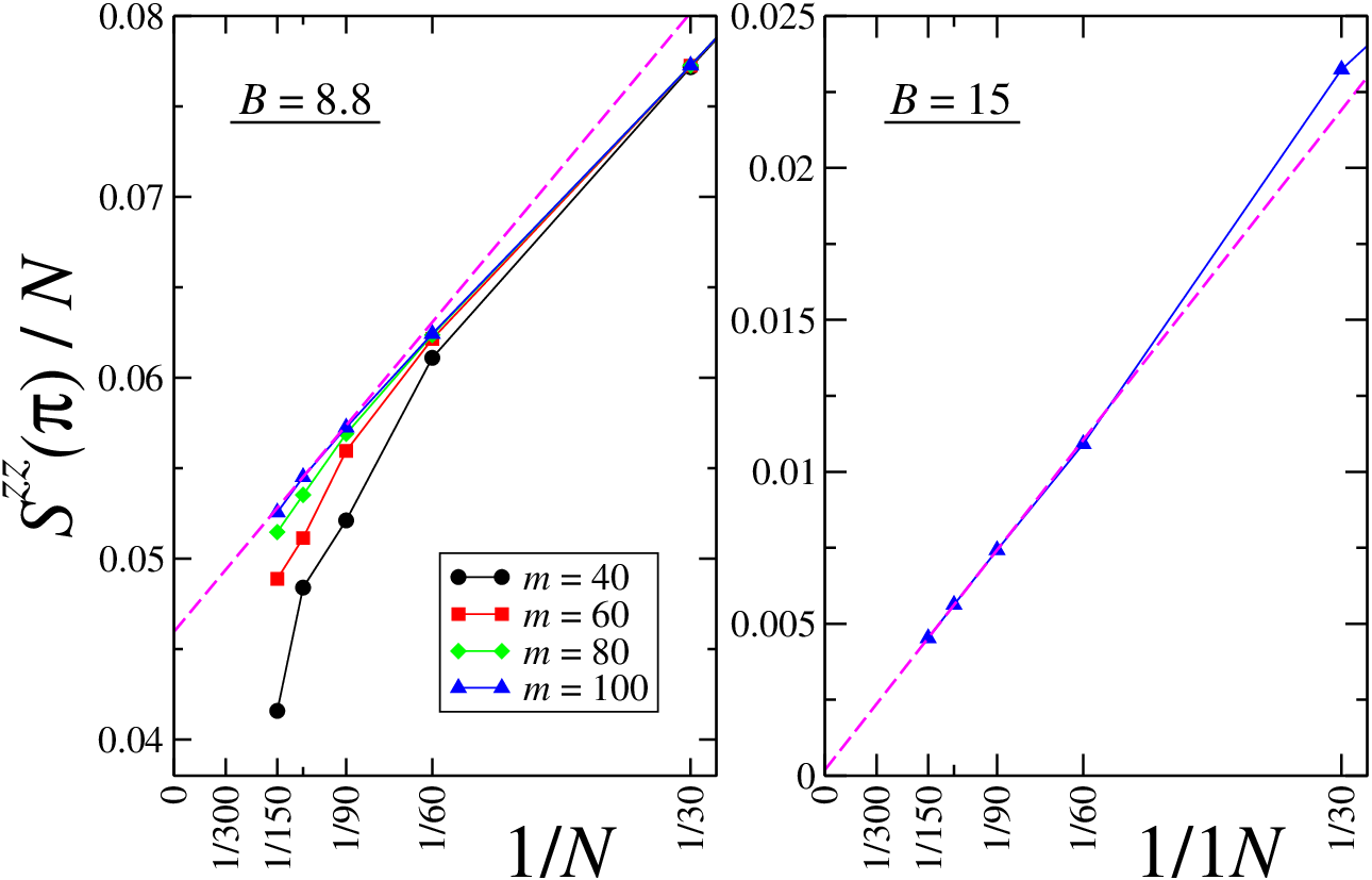

The calculation of the solid order required much larger MPS matrix dimensions. However, as already mentioned, since for large systems boundary effects are negligible when detecting the solid order, we computed by resorting to a standard variational MPS algorithm with OBC, where much larger values are attainable. To guarantee that our data are not qualitatively affected by boundary effects, we compared of Eq. (2) with the one evaluated by summing up only over a fraction of the spins corresponding to the central part of the chain (say, of the total length). The location of the phase transition point, where the solid order parameter drops from a finite to a vanishing value, do not change, even if the value of inside the solid phase can be different.
The results for the structure factor are reported in Fig. 4 for two emblematic cases. The left panel is obtained by setting and : it corresponds to a configuration which is well inside to the cusp of Fig. 2 of the supersolid phase. For these values the system should hence exhibits a non-null solid order parameter : this is clearly evident in the left panel of Fig. 4, where the value is found by extrapolating numerical data for from the linear behavior in of the quantity . [Notice that the solid ordering can be extracted only for , since at low the data accuracy rapidly deteriorates for larger sizes]. On the other hand, the right panel of Fig. 4 is obtained for and . It corresponds to a configuration which is far away from the supersolid region and for which the simulations of Ref. 9 predicted that no solid order should exist (indeed, the system is a superfluid there). This is confirmed by our simulations, where we observed in the thermodynamic limit, within numerical accuracy (Fig. 4, right panel).
Finally we observe that, for values of the anisotropy in Fig. 1, there is a direct transition from the supersolid to the superfluid phase. In this case the transition is detected by the vanishing of the solid order parameter. In Fig. 5 we show the spin structure factor as a function of the system size for different values of the external field, fixing . A scanning of this type for different values of allows to complete the boundaries of the supersolid phase.
In conclusion, we analyzed the supersolid phase in a one-dimensional anisotropic spin- Heisenberg model in a transverse magnetic field, and single-site uniaxial anisotropy. By means of an MPS variational calculation with PBC, we showed how to determine the spin-stiffness and the structure factor, such to locate the supersolid in the phase diagram of the system and find the critical exponent of the transition to the solid phase. For our model of interest, the resulting portion of the phase diagram containing the supersolid phase is shown in Fig. 1.
We acknowledge very fruitful discussions with S. Peotta, P. Sengupta, and P. Silvi. This work was supported by the FIRB-IDEAS project, RBID08B3FM, EU Projects IP-SOLID and ITNNANO.
References
- [1] A.F. Andreev and I.M. Lifshitz, Sov. Phys. JETP 29, 1107 (1969); A.J. Leggett, Phys. Rev. Lett. 25, 1543 (1970); H. Matsuda and T. Tsuneto, Suppl. Prog. Theor. Phys. 46, 411 (1970).
- [2] N. Prokof’ev, Adv. Phys. 56, 381 (2007).
- [3] E. Kim and M.H.N. Chan, Nature 427, 225 (2004).
- [4] T. Lahaye et al., Rep. Prog. Phys. 72, 126401 (2009); L. Pollet et al., Phys. Rev. Lett. 104, 125302 (2010); F. Cinti et al., Phys. Rev. Lett. 105, 135301 (2010).
- [5] K.-K. Ng and T. K. Lee, Phys. Rev. Lett. 97, 127204 (2006).
- [6] N. Laflorencie and F. Mila, Phys. Rev. Lett 99, 027202 (2007).
- [7] J.-D. Picon et al., Phys. Rev. B 78, 184418 (2008).
- [8] P. Sengupta and C.D. Batista, Phys. Rev. Lett. 98, 227201 (2007).
- [9] P. Sengupta and C.D. Batista, Phys. Rev. Lett. 99, 217205 (2007).
- [10] D. Peters, I.P. McCulloch, and W. Selke, Phys. Rev. B 79, 132406 (2009); J. Phys: Conf. Ser. 200 022046 (2010).
- [11] F. Verstraete, V. Murg, and J.I. Cirac, Adv. Phys. 57, 143 (2008).
- [12] F. Verstraete, D. Porras, and J.I. Cirac, Phys. Rev. Lett. 93, 227205 (2004).
- [13] A. W. Sandvik and G. Vidal, Phys. Rev. Lett. 99, 220602 (2007).
- [14] P. Pippan, S.R. White, and H.G. Evertz, Phys. Rev. B 81 081103(R) (2010).
- [15] B. Pirvu, F. Verstraete, and G. Vidal, Phys. Rev. B 83 125104 (2011).
- [16] D. Rossini, V. Giovannetti, and R. Fazio, arXiv:1102.3562
- [17] M.E. Fisher, M.N. Barber, and D. Jasnow, Phys. Rev. A 8, 1111 (1973).
- [18] The singular value decomposition of the product of a long chain of MPS transfer matrices (a matrix) typically has singular values rapidly decaying to zero. [14] For practical purposes, it is sufficient to take into account only of them, without compromising the accuracy (neglected values contribute with terms of the order of roundoff errors). In a similar fashion, the effective Hamiltonian on the MPS basis can be well approximated by expanding it via a singular value decomposition, keeping only the contributions associated to its largest eigenvalues.
- [19] For large values of and for , the model in Eq. (1) at low energies can be mapped onto an effective XX spin- chain in a transverse field, as shown in Ref. 9. We analytically extrapolated the critical exponent for such effective model after diagonalizing it in momentum space (in presence of a generic twist at the boundary). We found a theoretical value ; this agrees with the numerically computed value , within our accuracy.