跳到论文正文
W Papers独立论文阅读器 arXiv:1102.3487 论文正文 计算阅读时间 · 0%
引用这篇论文根据当前论文元数据生成,正式投稿前建议核对。


License: CC BY 3.0
arXiv:1102.3487v2 [hep-ph] 11 Feb 2012

Baryonium Study in Heavy Baryon Chiral Perturbation Theory

Yue-De Chen Note: Email: chenyuede-b07@mails.gucas.ac.cn    Cong-Feng QiaoOPENa)a) Department of Physics, Graduate University, the Chinese Academy of SciencesYuQuan Road 19A, 100049, Beijing, ChinaOPENb)b) Theoretical Physics Center for Science Facilities (TPCSF), CASYuQuan Road 19B, 100049, Beijing, China Note: Email: qiaocf@gucas.ac.cn

To see whether heavy baryon and anti-baryon can form a bound state, the heavy baryonium, we study the two-pion exchange interaction potential between them within the heavy baryon chiral perturbation theory. The obtained potential is applied to calculate the heavy baryonium masses by solving the Schrödinger equation. We find it is true that the heavy baryonium may exist in a reasonable choice of input parameters. The uncertainties remaining in the potential and their influences on the heavy baryonium mass spectrum are discussed.

1 Introduction

Quark model has achieved great success in describing the experimentally observed hadronic structures to a large extent. And the quark potential in between quark and anti-quark deduced from Chromodynamics (QCD) can explain the meson spectrum quite well. Many of predicted states by potential model were discovered in experiment and the theoretical predictions are in good agreement with experimental data, especially in charmonium and bottomonium sectors [1, 2, 3], where the masses of charm and bottom quarks are heavy enough to be treated non-relativistically. However, things became confused after the discovery of X⁡(3872)X(3872) in 2003 at Belle\mathrm{Belle} [4], which was later confirmed by BaBar\mathrm{BaBar} [5]. In recent years, a series of unusual states in charmonium sector, such as Y⁡(4260)Y(4260), Y⁡(4360)Y(4360), Y⁡(4660)Y(4660), and Z±​(4430)Z^{\pm}(4430), were observed in experiment [6]. Due to their extraordinary decay nature, it is hard to embed them into the conventional charmonium spectrum, which leads people to treat them as exotic rather than quark-quark bound states. The typical scenarios in explaining these newly found states include treating Y⁡(4260)Y(4260) as a hybrid charmonium [7], a χc​ρ0\chi_{c}\rho^{0} molecular state [8], a conventional Ψ⁡(4​S)\Psi(4S) [9], an ω​χc​1\omega\chi_{c1} molecular state [10], a Λc​Λ¯c\Lambda_{c}\bar{\Lambda}_{c} baryonium state [11], a D1​DD_{1}D or D0​D∗D_{0}D^{*} hadronic molecule [12], and a PP-wave tetraquark [c​s]​[c¯​s¯][cs][\bar{c}\bar{s}] state [13]; Y⁡(4360)Y(4360) is interpreted as the candidate of the charmonium hybrid or an excited D-wave charmonium state, the 33​D13^{3}D_{1} [14] and an excited state of baryonium [16]; Y⁡(4660)Y(4660) is suggested to be the excited S-wave charmonium states, the 53​S15^{3}S_{1} [14] and 63​S16^{3}S_{1} [15], a baryonium state [16, 17], a f0​(980)​Ψ′f_{0}(980)\Psi^{\prime} bound state [18, 19], a 53​S15^{3}S_{1}-43​D14^{3}D_{1} mixing state [20], and also a tetraquark state [21, 22]. There have been recently many research works on ”exotic” heavy quarkonium study in experiment and theory. To know more of recent progress in this respect and to have a more complete list of references one can see e.g. recent reviews [23, 24] and references therein.

In the baryonium picture, the tri-quark clusters are baryon-like, but not necessarily colorless. In the pioneer works of heavy baryonium for the interpretation of newly observed “exotic” structures [11, 16], there were only phenomenological and kinematic analysis, but without dynamics. In this work we attempt to study the heavy baryonium interaction potential arising from two-pion exchanges in the framework of Heavy Baryon Chiral Perturbation Theory (HBCPT) [25]. The paper is organized as follows. In Section 2, we present the formalism for the heavy baryon-baryon interaction study; in Section 3 we perform the numerical study for the mass spectrum of the possible baryonium with the obtained potential in preceding section; the Section 4 is devoted to the summary and conclusions. For the sake of reader’s convenience some of the used formulae are given in the Appendix.

2 Formalism

To obtain the heavy baryonium mass spectrum, we first start from extracting the baryon-baryon interaction potential in the same procedure as for quark-quark interaction [1].

2.1 Heavy Baryonium

In the heavy baryonium picture [16], Λc\Lambda_{c} and Σc0\Sigma^{0}_{c} are taken as basis vectors in two-dimensional space. The baryonia are loosely bound states of heavy baryon and anti-baryon, namely

B1+\displaystyle B^{+}_{1} ≡\displaystyle\equiv |Λc+Σ¯c0>\displaystyle|\Lambda_{c}^{+}\;\bar{\Sigma}_{c}^{0}>~~~~~~~~~
Triplet:B01\displaystyle{\rm Triplet:}\;\;\;\;\;B^{0}_{1} ≡\displaystyle\equiv 12(|Λc+Λ¯c+>−|Σc0Σ¯c0>)\displaystyle\frac{1}{\sqrt{2}}(|\Lambda_{c}^{+}\;\bar{\Lambda}_{c}^{+}>\;-\;|{\Sigma}_{c}^{0}\bar{\Sigma}_{c}^{0}>) (1)
B1−\displaystyle B^{-}_{1} ≡\displaystyle\equiv |Λ¯+cΣc0>\displaystyle|\bar{\Lambda}^{+}_{c}\;{\Sigma}_{c}^{0}>~~~~~~~~~

and

Singlet:B00≡12(|Λc+Λ¯c+>+|Σc0Σ¯c0>).\displaystyle{\rm Singlet:}\;\;\;\;\;B^{0}_{0}\equiv\frac{1}{\sqrt{2}}(|\Lambda_{c}^{+}\;\bar{\Lambda}_{c}^{+}>\;+\;|{\Sigma}_{c}^{0}\bar{\Sigma}_{c}^{0}>)\ . (2)

Here, approximately the transformation in this two-dimensional ”C-spin” space is invariant, which is in analog to the invariance of isospin transformation in proton and neutron system.

2.2 Effective Chiral Lagrangian

Heavy baryon contains both light and heavy quarks, of which the light component exhibits the chiral property and the heavy component exhibits heavy symmetry. Therefore, it is plausible to tackle the problem of heavy baryon interaction through the heavy chiral perturbation theory. Following we briefly review the gists of the HBCPT for later use.

In usual chiral perturbation theory, the nonlinear chiral symmetry is realized by making use of the unitary matrix

Σ=e2​i​Mfπ,\Sigma=e^{\frac{2iM}{f_{\pi}}}\;, (3)

where MM is a 3×33\times 3 matrix composed of eight Goldstone-boson fields, i.e.,

M=(12​π0+16​ηπ+K+π−−12​π0+16​ηK0K−K¯0−26​η).M=\left(\begin{array}[]{ccc}\frac{1}{\sqrt{2}}\pi^{0}+\frac{1}{\sqrt{6}}\eta&\phantom{+}\pi^{+}&\phantom{+}K^{+}\\ \phantom{+}\pi^{-}&-\frac{1}{\sqrt{2}}\pi^{0}+\frac{1}{\sqrt{6}}\eta&\phantom{+}K^{0}\\ \phantom{+}K^{-}&\phantom{+}\bar{K}^{0}&\phantom{+}-\frac{2}{\sqrt{6}}\eta\end{array}\right)\;. (4)

Here, fπf_{\pi} is the p​i​o​npion decay constant.

After the chiral symmetry spontaneously broken, the Goldstone boson interaction with hadron is introduced through a new matrix [26, 27]

ξ=Σ12=ei​Mfπ.\xi=\Sigma^{\frac{1}{2}}=e^{\frac{iM}{f_{\pi}}}\;. (5)

From ξ\xi one can construct a vector field VμV_{\mu} and an axial vector field AμA_{\mu} with simple chiral transformation properties, i.e.,

Vμ=12​(ξ†​∂μξ+ξ​∂μξ†),V_{\mu}=\frac{1}{2}(\xi^{{\dagger}}\partial_{\mu}\xi+\xi\partial_{\mu}\xi^{{\dagger}})\;, (6)
Aμ=i2​(ξ†​∂μξ−ξ​∂μξ†).A_{\mu}=\frac{i}{2}(\xi^{{\dagger}}\partial_{\mu}\xi-\xi\partial_{\mu}\xi^{{\dagger}})\;. (7)

For our aim, we work only on the leading order vector and axial vector fields in the expansion of ξ\xi in terms of fπf_{\pi}, they are

Vμ=1fπ2​M​∂μM,V_{\mu}=\frac{1}{f_{\pi}^{2}}M\partial_{\mu}M\;, (8)
Aμ=−1fπ∂μM.A_{\mu}=-\frac{1}{f_{\pi}}\partial_{\mu}M\;. (9)

For heavy baryon, each of the two light quarks is in a triplet of flavor SU(3), and hence the baryons can be grouped in two different SU(3) multiplets, the sixtet and antitriplet. The symmetric sixtet and antisymmetric triplet can be constructed out in 3×33\times 3 matrices [27], they are

B6=(Σc+⁣+12​Σc+12Ξc′+12​Σc+Σc012​Ξc0′12Ξc′+12​Ξc0′Ωc0),B_{6}=\left(\begin{array}[]{ccc}\Sigma_{c}^{++}&\frac{1}{\sqrt{2}}\Sigma_{c}^{+}&\frac{1}{\sqrt{2}}\Xi_{c}^{{}^{\prime}+}\\ \frac{1}{\sqrt{2}}\Sigma_{c}^{+}&\Sigma_{c}^{0}&\frac{1}{\sqrt{2}}\Xi_{c}^{{}^{\prime}0}\\ \frac{1}{\sqrt{2}}\Xi_{c}^{{}^{\prime}+}&\frac{1}{\sqrt{2}}\Xi_{c}^{{}^{\prime}0}&\Omega_{c}^{0}\end{array}\right)\;, (10)

and

B3¯=(0ΛcΞc+−Λc0Ξc−−Ξc+−Ξc−0),B_{\bar{3}}=\left(\begin{array}[]{ccc}0&\Lambda_{c}&\Xi_{c}^{+}\\ -\Lambda_{c}&0&\Xi_{c}^{-}\\ -\Xi_{c}^{+}&-\Xi_{c}^{-}&0\end{array}\right)\;, (11)

respectively.

Introducing six coupling constant gig_{i}, i=1,6i=1,6, the general chiral-invariant Lagrangian then reads [25]

ℒ𝒢\displaystyle\mathcal{L_{G}} =\displaystyle= 12tr[B¯3¯(iD/−M3¯)B3¯]+tr[B¯6(iD/−M6)B6]\displaystyle\frac{1}{2}tr[\bar{B}_{\bar{3}}(iD\!\!\!/-M_{\bar{3}})B_{\bar{3}}]+tr[\bar{B}_{6}(iD\!\!\!/-M_{6})B_{6}] (12)
+\displaystyle+ tr[B¯6∗μ[−gμ​ν(iD/−M6∗)+i(γμDν+γνDμ)−γμ(iD/+M6∗)γν]B6∗ν]\displaystyle tr[\bar{B}_{6}^{*\mu}[-g_{\mu\nu}(iD\!\!\!/-M_{6}^{*})+i(\gamma_{\mu}D_{\nu}+\gamma_{\nu}D_{\mu})-\gamma_{\mu}(iD\!\!\!/+M_{6}^{*})\gamma_{\nu}]B_{6}^{*\nu}]
+\displaystyle+ g1​t​r​(B¯6​γμ​γ5​Aμ​B6)+g2​t​r​(B¯6​γμ​γ5​Aμ​B3¯)+h.c.\displaystyle g_{1}tr(\bar{B}_{6}\gamma_{\mu}\gamma_{5}A^{\mu}B_{6})+g_{2}tr(\bar{B}_{6}\gamma_{\mu}\gamma_{5}A^{\mu}B_{\bar{3}})+h.c.
+\displaystyle+ g3​t​r​(B¯6​μ∗​Aμ​B6)+h.c.+g4​t​r​(B¯6​μ∗​Aμ​B3¯)+h.c.\displaystyle g_{3}tr(\bar{B}_{6{\mu}}^{*}A^{\mu}B_{6})+h.c.+g_{4}tr(\bar{B}_{6{\mu}}^{*}A^{\mu}B_{\bar{3}})+h.c.
+\displaystyle+ g5tr(B¯6ν∗γμγ5AμB6​ν∗)+g6tr(B¯3¯γμγ5AμB3¯).\displaystyle g_{5}tr(\bar{B}_{6}^{\nu*}\gamma_{\mu}\gamma_{5}A^{\mu}B_{6\nu}^{*})+g_{6}tr(\bar{B}_{\bar{3}}\gamma_{\mu}\gamma_{5}A^{\mu}B_{\bar{3}})\;.

Here, B6​ν∗B_{6\nu}^{*} is a Rarita-Schwinger vector-spinor field for spin-32\frac{3}{2} particle; M3¯M_{\bar{3}}, M6M_{6}, M6∗M_{6}^{*} represent for heavy baryon mass matrices of corresponding fields; With the help of vector current VμV_{\mu} defined in Eq. (8), we may construct the covariant derivative DμD_{\mu}, which acts on baryon field, as

Dμ​B6=∂μB6+Vμ​B6+B6​VμT,D_{\mu}B_{6}=\partial_{\mu}B_{6}+V_{\mu}B_{6}+B_{6}V_{\mu}^{T}\;, (13)
Dμ​B3¯=∂μB3¯+Vμ​B3¯+B3¯​VμT,D_{\mu}B_{\bar{3}}=\partial_{\mu}B_{\bar{3}}+V_{\mu}B_{\bar{3}}+B_{\bar{3}}V_{\mu}^{T}\;, (14)

where VμTV_{\mu}^{T} stands for the transpose of VμV_{\mu}. Thus, the couplings of vector current to heavy baryons relevant to our task take the following form

ℒℰ1\displaystyle\mathcal{L}_{{\mathcal{E}_{1}}} =\displaystyle= 12​t​r​(B¯3¯​i​γμ​Vμ​B3¯)\displaystyle\frac{1}{2}tr(\bar{B}_{\bar{3}}i\gamma^{\mu}V_{\mu}B_{\bar{3}}) (15)
=\displaystyle= 12​fπ2​Λ¯c​i​γμ​(π0​∂μπ0+π−​∂μπ++π+​∂μπ−)​Λc,\displaystyle\frac{1}{2f_{\pi}^{2}}\bar{\Lambda}_{c}i\gamma^{\mu}(\pi^{0}\partial_{\mu}\pi^{0}+\pi^{-}\partial_{\mu}\pi^{+}+\pi^{+}\partial_{\mu}\pi^{-})\Lambda_{c}\;,

and

ℒℰ2\displaystyle\mathcal{L}_{{\mathcal{E}_{2}}} =\displaystyle= 12​t​r​(B¯3¯​B3¯​i​γμ​VμT)\displaystyle\frac{1}{2}tr(\bar{B}_{\bar{3}}B_{\bar{3}}i\gamma^{\mu}V_{\mu}^{T}) (16)
=\displaystyle= 12​fπ2​Λ¯c​Λc​i​γμ​(π0​∂μπ0+π−​∂μπ++π+​∂μπ−).\displaystyle\frac{1}{2f_{\pi}^{2}}\bar{\Lambda}_{c}\Lambda_{c}i\gamma^{\mu}(\pi^{0}\partial_{\mu}\pi^{0}+\pi^{-}\partial_{\mu}\pi^{+}+\pi^{+}\partial_{\mu}\pi^{-})\;.

According to the heavy quark symmetry, there are four constraint relations among those six coupling constants of the Lagrangian of Eq. (12), i.e.,

g6=0,g3=32​g1,g5=−32​g1,g4=−3​g2,\displaystyle g_{6}=0\;,\;g_{3}=\frac{\sqrt{3}}{2}g_{1}\;,\;g_{5}=-\frac{3}{2}g_{1}\;,\;g_{4}=-\sqrt{3}g_{2}\;, (17)

which means the number of independent couplings are then reduced to two. In this work, we employ g1g_{1} and g2g_{2} for the numerical evaluation as did in Ref. [25].

Here, to get the dominant interaction potential we restrict our effort only on the p​i​o​npion exchange processes as usual. Notice that the couplings of p​i​o​npion to spin-32\frac{3}{2} and -12\frac{1}{2} baryons, and p​i​o​npion to two spin-12\frac{1}{2} baryons take a similar form, in the following we merely present the spin-32\frac{3}{2} and -12\frac{1}{2} baryon-p​i​o​npion coupling for illustration, i.e.,

ℒ1=g32​fπ​Σc¯0∗μ​∂μπ0​Σc0+h.c.,\mathcal{L}_{1}=\frac{g_{3}}{\sqrt{2}f_{\pi}}\bar{\Sigma_{c}}\!^{0*\mu}\partial_{\mu}\pi^{0}\Sigma_{c}^{0}+h.c.\;, (18)
ℒ2=−g32​fπΣc¯+∗μ∂μπ+Σc0+h.c.,\mathcal{L}_{2}=-\frac{g_{3}}{\sqrt{2}f_{\pi}}\bar{\Sigma_{c}}\!^{+*\mu}\partial_{\mu}\pi^{+}\Sigma_{c}^{0}+h.c.\;, (19)
ℒ3=g4fπΣc¯++∗μ∂μπ+Λc++h.c.,\mathcal{L}_{3}=\frac{g_{4}}{f_{\pi}}\bar{\Sigma_{c}}\!^{++*\mu}\partial_{\mu}\pi^{+}\Lambda_{c}^{+}+h.c.\;, (20)
ℒ4=−g4fπΣc¯0∗μ∂μπ−Λc++h.c.,\mathcal{L}_{4}=-\frac{g_{4}}{f_{\pi}}\bar{\Sigma_{c}}\!^{0*\mu}\partial_{\mu}\pi^{-}\Lambda_{c}^{+}+h.c.\;, (21)
ℒ5=−g4fπΣc¯+∗μ∂μπ0Λc++h.c..\mathcal{L}_{5}=-\frac{g_{4}}{f_{\pi}}\bar{\Sigma_{c}}\!^{+*\mu}\partial_{\mu}\pi^{0}\Lambda_{c}^{+}+h.c.\;. (22)

To get the p​i​o​npion and two spin-12\frac{1}{2} baryon couplings one only needs to replace the Σc∗μ\Sigma_{c}^{*\mu} by Σc\Sigma_{c}, g3g_{3} by g1g_{1}, g4g_{4} by g2g_{2}, and insert γμ​γ5\gamma^{\mu}\gamma_{5} in between the two baryon fields in Eqs.(18)-(22).

Refer to caption
Refer to caption
Figure 1: Schematic Diagrams which contribute to the baryonium potential.

2.3 Baryonium Potential from Two-pion Exchange

To obtain heavy baryon-baryon interaction potential in configuration space, we start from writing down the two-body scattering amplitude in the center-of-mass frame(CMS), i.e. taking pa=−pb\textbf{p}_{a}=-\textbf{p}_{b} and pa′=−pb′\textbf{p}_{a}^{\prime}=-\textbf{p}_{b}^{\prime}. In CMS the total and relative four momenta are defined as

P\displaystyle P =\displaystyle= (pa+pb)=(pa′+pb′)=(E, 0),\displaystyle(p_{a}\;+\;p_{b})\;=\;(p_{a}^{\prime}\;+\;p_{b}^{\prime})=(E,\;0)\;, (23)
p\displaystyle p =\displaystyle= 12​(pa−pb)=(0,p),\displaystyle\frac{1}{2}(p_{a}\;-\;p_{b})\;=\;(0,\;\textbf{p})\;, (24)
p′\displaystyle p^{\prime} =\displaystyle= 12​(pa′−pb′)=(0,p′).\displaystyle\frac{1}{2}(p_{a}^{\prime}\;-\;p_{b}^{\prime})\;=\;(0,\;\textbf{p}^{\prime})\;. (25)

To perform the calculation, it is convenient to introduce some new variables as functions of p and p′\textbf{p}^{\prime}, i.e.,

𝒲⁡(p)\displaystyle\mathcal{W}(\textbf{p}) =Ea​(p)+Eb​(p),\displaystyle=E_{a}(\textbf{p})+E_{b}(\textbf{p})\;, (26)
𝒲⁡(p′)\displaystyle\mathcal{W}(\textbf{p}^{\prime}) =Ea​(p′)+Eb​(p′),\displaystyle=E_{a}(\textbf{p}^{\prime})+E_{b}(\textbf{p}^{\prime})\;, (27)
FE​(p,p0)\displaystyle F_{E}(\textbf{p},\;p_{0}) =12​E+p0−E⁡(p)+i​δ,\displaystyle=\frac{1}{2}E+p_{0}-E(\textbf{p})+i\delta\;, (28)

where δ\delta is an infinitesimal quantity introduced in the so-called i​δi\delta prescription. Following the same procedure as in Refs. [28, 29], it is straightforward to write down the baryon-baryon scattering kernels, shown as box and crossed diagrams in Figure 1,

Kb​o​x=\displaystyle K_{box}= −\displaystyle- 1(2​π)2​(E−𝒲⁡(p′))​(E−𝒲⁡(p))​∫d​p0′​d​p0​d​k20​d​k10​d3​k2​d3​k1\displaystyle\frac{1}{(2\pi)^{2}}(E-\mathcal{W}(\textbf{p}^{\prime}))(E-\mathcal{W}(\textbf{p}))\int dp_{0}^{\prime}dp_{0}dk_{20}dk_{10}d^{3}\textbf{k}_{2}d^{3}\textbf{k}_{1} (29)
×\displaystyle\times i(2​π)4​δ4​(p−p′−k1−k2)​1k22−m2+i​δ​1FE​(p′,p0′)​FE​(−p′,−p0′)\displaystyle\frac{i}{(2\pi)^{4}}\delta^{4}(p-p^{\prime}-k_{1}-k_{2})\frac{1}{k_{2}^{2}-m^{2}+i\delta}\frac{1}{F_{E}(\textbf{p}^{\prime},p_{0}^{\prime})F_{E}(-\textbf{p}^{\prime},-p_{0}^{\prime})}
×\displaystyle\times Γj​Γi​Γi​ΓjFE​(p−k,p0−k10)​FE​(−p+k,−p0+k10)​1OPENFE​(p,p0)​FE​(p,−p0))\displaystyle\frac{\Gamma_{j}\Gamma_{i}\Gamma_{i}\Gamma_{j}}{F_{E}(\textbf{p}-\textbf{k},p_{0}-k_{10})F_{E}(-\textbf{p}+\textbf{k},-p_{0}+k_{10})}\frac{1}{F_{E}(\textbf{p},p_{0})F_{E}(\textbf{p},-p_{0}))}
×\displaystyle\times 1k12−m2+i​δ,\displaystyle\frac{1}{k_{1}^{2}-m^{2}+i\delta}\;,
Kc​r​o​s​s=\displaystyle K_{cross}= −\displaystyle- 1(2​π)2​(E−𝒲⁡(p′))​(E−𝒲⁡(p))​∫d​p0′​d​p0​d​k20​d​k10​d3​k2​d3​k1\displaystyle\frac{1}{(2\pi)^{2}}(E-\mathcal{W}(\textbf{p}^{\prime}))(E-\mathcal{W}(\textbf{p}))\int dp_{0}^{\prime}dp_{0}dk_{20}dk_{10}d^{3}\textbf{k}_{2}d^{3}\textbf{k}_{1} (30)
×\displaystyle\times i(2​π)4​δ4​(p−p′−k1−k2)​1k22−m2+i​δ​1FE​(p′,p0′)​FE​(−p′,−p0′)\displaystyle\frac{i}{(2\pi)^{4}}\delta^{4}(p-p^{\prime}-k_{1}-k_{2})\frac{1}{k_{2}^{2}-m^{2}+i\delta}\frac{1}{F_{E}(\textbf{p}^{\prime},p_{0}^{\prime})F_{E}(-\textbf{p}^{\prime},-p_{0}^{\prime})}
×\displaystyle\times Γj​Γi​Γj​ΓiFE​(p−k,p0−k10)​FE​(−p′−k,−p0′−k10)​1FE​(p,p0)​FE​(−p,−p0)\displaystyle\frac{\Gamma_{j}\Gamma_{i}\Gamma_{j}\Gamma_{i}}{F_{E}(\textbf{p}-\textbf{k},p_{0}-k_{10})F_{E}(-\textbf{p}^{\prime}-\textbf{k},-p_{0}^{\prime}-k_{10})}\frac{1}{F_{E}(\textbf{p},p_{0})F_{E}(-\textbf{p},-p_{0})}
×\displaystyle\times 1k12−m2+i​δ.\displaystyle\frac{1}{k_{1}^{2}-m^{2}+i\delta}\;.

Here, mm corresponds to the p​i​o​npion mass and Γi,j\Gamma_{i,j} are heavy baryon-p​i​o​npion interaction vertices that can be read out from the Lagrangian in Eqs.(18)-(22). In case of spin-32\frac{3}{2} intermediate,

Γj​Γi​Γi​Γj\displaystyle\Gamma_{j}\Gamma_{i}\Gamma_{i}\Gamma_{j} =\displaystyle= (g4fπ)4​u¯​(−p)​k2μ​uμ​(p−k1)​u¯ν​(p−k1)​k1ν​u​(p)\displaystyle\left(\frac{g_{4}}{f_{\pi}}\right)^{4}\bar{u}(-p)k_{2}^{\mu}u_{\mu}(p-k_{1})\bar{u}_{\nu}(p-k_{1})k_{1}^{\nu}u(p) (31)
×\displaystyle\times v¯​(p)​(−k1α)​vα​(−p+k1)​v¯β​(−p+k1)​k2β​v​(−p),\displaystyle\bar{v}(p)(-k_{1}^{\alpha})v_{\alpha}(-p+k_{1})\bar{v}_{\beta}(-p+k_{1})k_{2}^{\beta}v(-p)\;,

and in case of spin-12\frac{1}{2} intermediate

Γj​Γi​Γi​Γj\displaystyle\Gamma_{j}\Gamma_{i}\Gamma_{i}\Gamma_{j} =\displaystyle= (g2fπ)4​u¯​(−p)​γμ​γ5​k2μ​u​(p−k1)​u¯​(p−k1)​γν​γ5​k1ν​u​(p)\displaystyle\left(\frac{g_{2}}{f_{\pi}}\right)^{4}\bar{u}(-p)\gamma_{\mu}\gamma_{5}k_{2}^{\mu}u(p-k_{1})\bar{u}(p-k_{1})\gamma_{\nu}\gamma_{5}k_{1}^{\nu}u(p) (32)
×\displaystyle\times v¯​(p)​γα​γ5​(−k1α)​v​(−p+k1)​v¯​(−p+k1)​γβ​γ5​k2β​v​(−p).\displaystyle\bar{v}(p)\gamma_{\alpha}\gamma_{5}(-k_{1}^{\alpha})v(-p+k_{1})\bar{v}(-p+k_{1})\gamma_{\beta}\gamma_{5}k_{2}^{\beta}v(-p)\;.

Integrating over p0′p^{\prime}_{0}, p0p_{0}, k10k_{10}, and k20k_{20} in Eq.(29) one obtains the interaction kernel of box diagram at order 𝒪⁡(1MH)\mathcal{O}(\frac{1}{M_{H}}),

Kb​o​x=\displaystyle K_{box}= −\displaystyle- 1(2​π)3​∫d3​k1​d3​k24​Ek1​Ek2​Γj​ΓiEp−k1+Ep−W+Ek1\displaystyle\frac{1}{(2\pi)^{3}}\int\frac{d^{3}\textbf{k}_{1}d^{3}\textbf{k}_{2}}{4E_{\textbf{k}_{1}}E_{\textbf{k}_{2}}}\frac{\Gamma_{j}\Gamma_{i}}{E_{\textbf{p}-\textbf{k}_{1}}+E_{\textbf{p}}-W+E_{\textbf{k}_{1}}} (33)
×\displaystyle\times Γi​ΓjEp′+Ep−k1−W+Ek2​1Ep+Ep′−W+Ek1+Ek2,\displaystyle\frac{\Gamma_{i}\Gamma_{j}}{E_{\textbf{p}}^{\prime}+E_{\textbf{p}-\textbf{k}_{1}}-W+E_{\textbf{k}_{2}}}\frac{1}{E_{\textbf{p}}+E_{\textbf{p}^{\prime}}-W+E_{\textbf{k}_{1}}+E_{\textbf{k}_{2}}}\;,

where MHM_{H} represents one of the heavy baryon mass, MΛc+M_{\Lambda_{c}^{+}}, MΣc0M_{\Sigma^{0}_{c}} or MΣc∗M_{\Sigma_{c}^{*}}; Ep−k1=(p−k1)2+MΣc∗2E_{\textbf{p}-\textbf{k}_{1}}=\sqrt{(\textbf{p}-\textbf{k}_{1})^{2}+M_{\Sigma_{c}^{*}}^{2}} is the intermediate state energy; Ek1=k12+m2E_{\textbf{k}_{1}}=\sqrt{\textbf{k}_{1}^{2}+m^{2}} and Ek2=k22+m2E_{\textbf{k}_{2}}=\sqrt{\textbf{k}_{2}^{2}+m^{2}} are two 𝑝𝑖𝑜𝑛\it{pion}s’ energies; and W=2​E​(p)W=2E(\textbf{p}). With the same procedure, we can get the interaction kernel of crossed diagram, i.e.

Kc​r​o​s​s=\displaystyle K_{cross}= −\displaystyle- 1(2​π)3​∫d3​k1​d3​k24​Ek1​Ek2​Γj​ΓiEp−k1+Ep−W+Ek1\displaystyle\frac{1}{(2\pi)^{3}}\int\frac{d^{3}\textbf{k}_{1}d^{3}\textbf{k}_{2}}{4E_{\textbf{k}_{1}}E_{\textbf{k}_{2}}}\frac{\Gamma_{j}\Gamma_{i}}{E_{\textbf{p}-\textbf{k}_{1}}+E_{\textbf{p}}-W+E_{\textbf{k}_{1}}} (34)
×\displaystyle\times Γj​ΓiEp′+Ep′+k1−W+Ek1​1Ep+Ep′−W+Ek1+Ek2.\displaystyle\frac{\Gamma_{j}\Gamma_{i}}{E_{\textbf{p}}^{\prime}+E_{\textbf{p}^{\prime}+\textbf{k}_{1}}-W+E_{\textbf{k}_{1}}}\frac{1}{E_{\textbf{p}}+E_{\textbf{p}^{\prime}}-W+E_{\textbf{k}_{1}}+E_{\textbf{k}_{2}}}\;.

Next, since what we are interested in is the heavy baryons, we can further implement the non-relativistic reduction on spinors with the help of vertices given in Eqs.(18)-(22). In the end, the non-relativistic reduction for Λc+​Σc+⁣∗​π0\Lambda_{c}^{+}\Sigma_{c}^{+*}\pi^{0} and Λc+​Σc+​π0\Lambda_{c}^{+}\Sigma_{c}^{+}\pi^{0} couplings gives

i(g4fπ)u¯(p2)uμ(p1)(p2−p1)μ=−i(g4fπ)S†⋅q,i\left(\frac{g_{4}}{f_{\pi}}\right)\bar{u}(p_{2})u_{\mu}(p_{1})(p_{2}-p_{1})^{\mu}=-i\left(\frac{g_{4}}{f_{\pi}}\right)\textbf{S}^{{\dagger}}\cdot\textbf{q}\;, (35)

and

i⁡(g2fπ)​u¯​(p2)​γμ​γ5​u​(p1)​(p2−p1)μ=i⁡(g2fπ)​𝝈1⋅q,i\left(\frac{g_{2}}{f_{\pi}}\right)\bar{u}(p_{2})\gamma_{\mu}\gamma_{5}u(p_{1})(p_{2}-p_{1})^{\mu}=i\left(\frac{g_{2}}{f_{\pi}}\right)\boldsymbol{\sigma}_{1}\cdot\textbf{q}\;, (36)

respectively. Here, q=p2−p1\textbf{q}=\textbf{p}_{2}-\textbf{p}_{1} and S†\textbf{S}^{{\dagger}} is the spin-12\frac{1}{2} to spin-32\frac{3}{2} transition operator.

In the process of deriving Λc+−Λ¯c+\Lambda_{c}^{+}-\bar{\Lambda}_{c}^{+} potential, the Σc+\Sigma_{c}^{+} and Σc+⁣∗\Sigma_{c}^{+*} are taken into account as intermediate states. Using Eqs. (35)-(36) and the explicit forms of spinors given in the appendix, we can readily obtain the reduction forms for the Σc+\Sigma_{c}^{+} intermediate

u¯(−p)γμγ5k2μu(p−k1)u¯(p−k1)γνγ5k1νu(p)×\displaystyle\bar{u}(-p)\gamma_{\mu}\gamma_{5}k_{2}^{\mu}u(p-k_{1})\bar{u}(p-k_{1})\gamma_{\nu}\gamma_{5}k_{1}^{\nu}u(p)\times (37)
v¯​(p)​γα​γ5​(−k1α)​v​(−p+k1)​v¯​(−p+k1)​γβ​γ5​k2β​v​(−p)\displaystyle\bar{v}(p)\gamma_{\alpha}\gamma_{5}(-k_{1}^{\alpha})v(-p+k_{1})\bar{v}(-p+k_{1})\gamma_{\beta}\gamma_{5}k_{2}^{\beta}v(-p)
=\displaystyle= (k1⋅k2)2+(𝝈1⋅k1×k2)​(𝝈2⋅k1×k2),\displaystyle(\textbf{k}_{1}\cdot\textbf{k}_{2})^{2}+(\boldsymbol{\sigma}_{1}\cdot\textbf{k}_{1}\times\textbf{k}_{2})(\boldsymbol{\sigma}_{2}\cdot\textbf{k}_{1}\times\textbf{k}_{2})\;,

the Σc+⁣∗\Sigma_{c}^{+*} intermediate in the box diagram

u¯(−p)k2μuμ(p−k1)u¯ν(p−k1)k1νu(p)×\displaystyle\bar{u}(-p)k_{2}^{\mu}u_{\mu}(p-k_{1})\bar{u}_{\nu}(p-k_{1})k_{1}^{\nu}u(p)\times (38)
v¯​(p)​(−k1α)​vα​(−p+k1)​v¯β​(−p+k1)​k2β​v​(−p)\displaystyle\bar{v}(p)(-k_{1}^{\alpha})v_{\alpha}(-p+k_{1})\bar{v}_{\beta}(-p+k_{1})k_{2}^{\beta}v(-p)
=\displaystyle= 49​(k1⋅k2)2−19​(𝝈1⋅k1×k2)​(𝝈2⋅k1×k2),\displaystyle\frac{4}{9}(\textbf{k}_{1}\cdot\textbf{k}_{2})^{2}-\frac{1}{9}(\boldsymbol{\sigma}_{1}\cdot\textbf{k}_{1}\times\textbf{k}_{2})(\boldsymbol{\sigma}_{2}\cdot\textbf{k}_{1}\times\textbf{k}_{2})\;,

and the crossed diagram

u¯(−p)k2μuμ(p−k1)u¯ν(p−k1)k1νu(p)×\displaystyle\bar{u}(-p)k_{2}^{\mu}u_{\mu}(p-k_{1})\bar{u}_{\nu}(p-k_{1})k_{1}^{\nu}u(p)\times (39)
v¯​(p)​(−k1α)​vα​(−p+k1)​v¯β​(−p+k1)​k2β​v​(−p)\displaystyle\bar{v}(p)(-k_{1}^{\alpha})v_{\alpha}(-p+k_{1})\bar{v}_{\beta}(-p+k_{1})k_{2}^{\beta}v(-p)
=\displaystyle= 49​(k1⋅k2)2+19​(𝝈1⋅k1×k2)​(𝝈2⋅k1×k2),\displaystyle\frac{4}{9}(\textbf{k}_{1}\cdot\textbf{k}_{2})^{2}+\frac{1}{9}(\boldsymbol{\sigma}_{1}\cdot\textbf{k}_{1}\times\textbf{k}_{2})(\boldsymbol{\sigma}_{2}\cdot\textbf{k}_{1}\times\textbf{k}_{2})\;,

respectively. Thus, the spinor reduction finally leads to an operator 𝒪1​(k1,k2)\mathcal{O}_{1}(\textbf{k}_{1},\;\textbf{k}_{2}), of which the variables k1\textbf{k}_{1} and k2\textbf{k}_{2} can be replaced by gradient operators ∇1\boldsymbol{\nabla}_{1} and ∇2\boldsymbol{\nabla}_{2} in configuration space and acting on r1\textbf{r}_{1} and r2\textbf{r}_{2}, respectively. This operator is expressed as

𝒪1​(k1,k2)\displaystyle\mathcal{O}_{1}(\textbf{k}_{1},\;\textbf{k}_{2}) =\displaystyle= c1​O1​(k1,k2)+c2​O2​(k1,k2)\displaystyle c_{1}O_{1}(\textbf{k}_{1},\;\textbf{k}_{2})+c_{2}O_{2}(\textbf{k}_{1},\;\textbf{k}_{2}) (40)
=\displaystyle= c1​(k1⋅k2)2+c2​(𝝈1⋅k1×k2)​(𝝈2⋅k1×k2).\displaystyle c_{1}(\textbf{k}_{1}\cdot\textbf{k}_{2})^{2}+c_{2}(\boldsymbol{\sigma}_{1}\cdot\textbf{k}_{1}\times\textbf{k}_{2})(\boldsymbol{\sigma}_{2}\cdot\textbf{k}_{1}\times\textbf{k}_{2})\;.

Here, the decomposition coefficients c1c_{1} and c2c_{2} are given in Table 1. The first part of Eq. (40) may generate the central potential and the second part may generate the spin-spin coupling and the tensor potentials, which are explicitly shown in the Appendix.

Table 1: The values of coefficients c1c_{1} and c2c_{2} in the decomposition of operator O⁡(k1,k2)O(\textbf{k}_{1},\;\textbf{k}_{2}) in Eq. (40). The left one is for the spin-12\frac{1}{2} intermediate state case and the right one is for the spin-32\frac{3}{2} case.
spin-1/2 c1~c_{1} c2~c_{2}
box  1  1
cross  1  1
spin-3/2 c1c_{1} c2c_{2}
box 4/94/9 −1/9-1/9
cross 4/94/9 1/9~~1/9

To get the leading order central potential, e.g. for Λc\Lambda_{c}-Λ¯c\bar{\Lambda}_{c} system, we first expand the energy in powers of 1MH\frac{1}{M_{H}}, but keep only the leading term, like

1Ep−k1+Ep−W+Ek1\displaystyle\frac{1}{E_{\textbf{p}-\textbf{k}_{1}}+E_{\textbf{p}}-W+E_{\textbf{k}_{1}}} ≈\displaystyle\approx 1MΣc∗+MΛc−2​MΛc+Ek1=1Ek1+Δ1,\displaystyle\frac{1}{M_{\Sigma_{c}^{*}}+M_{\Lambda_{c}}-2M_{\Lambda_{c}}+E_{\textbf{k}_{1}}}=\frac{1}{E_{\textbf{k}_{1}}+\Delta_{1}}, (41)

where Δ1=MΣc∗−MΛc\Delta_{1}=M_{\Sigma_{c}^{*}}-M_{\Lambda_{c}} represents the mass splitting. By virtue of the factorization in integrals given in the Appendix, we can then make a double Fourier transformation, i.e.,

VCB(r1,r2)=−(g44fπ4)∫∫d3​k1​d3​k2(2​π)6𝒪1​(k1,k2)​ei​k1​r1​ei​k2​r2​f​(k12)​f​(k22)2​Ek1​Ek2​(Ek1+Δ1)​(Ek2+Δ1)​(Ek1+Ek2),\displaystyle V_{C}^{B}(r_{1},\;r_{2})=-\left(\frac{g_{4}^{4}}{f_{\pi}^{4}}\right)\int\int\frac{d^{3}\textbf{k}_{1}d^{3}\textbf{k}_{2}}{(2\pi)^{6}}\frac{\mathcal{O}_{1}(\textbf{k}_{1},\textbf{k}_{2})e^{i\textbf{k}_{1}\textbf{r}_{1}}e^{i\textbf{k}_{2}\textbf{r}_{2}}f(\textbf{k}_{1}^{2})f(\textbf{k}_{2}^{2})}{2E_{\textbf{k}_{1}}E_{\textbf{k}_{2}}(E_{\textbf{k}_{1}}+\Delta_{1})(E_{\textbf{k}_{2}}+\Delta_{1})(E_{\textbf{k}_{1}}+E_{\textbf{k}_{2}})}\;, (42)

where the superscript BB denotes the box diagram and the subscript CC means central potential. Similarly, one can get the central potential from the crossed diagram contribution

VCC(r1,r2)=−(g44fπ4)∫∫d3​k1​d3​k2(2​π)6𝒪1(k1,k2)ei​k1​r1ei​k2​r2f(k12)f(k22)D,V_{C}^{C}(r_{1},\;r_{2})=-\left(\frac{g_{4}^{4}}{f_{\pi}^{4}}\right)\int\int\frac{d^{3}\textbf{k}_{1}d^{3}\textbf{k}_{2}}{(2\pi)^{6}}\mathcal{O}_{1}(\textbf{k}_{1},\textbf{k}_{2})e^{i\textbf{k}_{1}\textbf{r}_{1}}e^{i\textbf{k}_{2}\textbf{r}_{2}}f(\textbf{k}_{1}^{2})f(\textbf{k}_{2}^{2})\ D\;, (43)

where the superscript CC denote crossed diagram and the subscript CC means central potential, and

D\displaystyle D =\displaystyle= 14​Ek1​Ek2[(1(Ek1+Δ1)2+1(Ek2+Δ1)2)1Ek1+Ek2\displaystyle\!\!\!\frac{1}{4E_{\textbf{k}_{1}}E_{\textbf{k}_{2}}}\left[\left(\frac{1}{(E_{\textbf{k}_{1}}+\Delta_{1})^{2}}+\frac{1}{(E_{\textbf{k}_{2}}+\Delta_{1})^{2}}\right)\frac{1}{E_{\textbf{k}_{1}}+E_{\textbf{k}_{2}}}\right. (44)
+\displaystyle+ (1(Ek1+Δ1)2+1(Ek2+Δ1)2+2(Ek1+Δ1)​(Ek2+Δ1))1Ek1+Ek2+2​Δ1].\displaystyle\!\!\!\left(\frac{1}{(E_{\textbf{k}_{1}}+\Delta_{1})^{2}}\left.+\frac{1}{(E_{\textbf{k}_{2}}+\Delta_{1})^{2}}+\frac{2}{(E_{\textbf{k}_{1}}+\Delta_{1})(E_{\textbf{k}_{2}}+\Delta_{1})}\right)\frac{1}{E_{\textbf{k}_{1}}+E_{\textbf{k}_{2}}+2\Delta_{1}}\right].

In order to regulate the potentials we have introduced form factors at each baryon-pion vertex. The resulting f⁡(𝐤𝟐)f(\bf k^{2}) form factors appearing in Eqs. (42) and (43) will be given in Section 3.

Taking a similar approach as given in above one can readily get the central potential in other interaction channels and also the tensor potential. Notice that although there exists the one-pion exchange contribution in Σc\Sigma_{c}-Σc\Sigma_{c} system, due to the γμ​γ5\gamma_{\mu}\gamma_{5} nature in interaction vertex, it only contributes to 𝝈1⋅𝝈2\boldsymbol{\sigma}_{1}\cdot\boldsymbol{\sigma}_{2} term, which is out of our concern in this work. Here we just focus on the central potential.

Refer to caption
Refer to caption
Figure 2: The triangle and two-pion loop diagrams.

Besides box and crossed diagrams, there are also contributions from triangle and two-pion loop diagrams as shown in Fig. 2. As in the box and crossed diagrams, after integrating over energy component, we get the pion-pair contribution, as shown in the left diagram of Figure 2, as [33]

Vt​r​i​a​n​g​l​e​(r1,r2)=g422​fπ4​∫∫d3​k1​d3​k2(2​π)6​𝒪2​(k1,k2)​(Ek1+Ek2)​ei​k1​r1​ei​k2​r2​f​(k12)​f​(k22)Ek1​Ek2​(Ek1+Δ1)​(Ek2+Δ1),V_{triangle}(r_{1},r_{2})=\frac{g_{4}^{2}}{2f_{\pi}^{4}}\int\int\frac{d^{3}\textbf{k}_{1}d^{3}\textbf{k}_{2}}{(2\pi)^{6}}\frac{\mathcal{O}_{2}(\textbf{k}_{1},\textbf{k}_{2})(E_{\textbf{k}_{1}}+E_{\textbf{k}_{2}})e^{i\textbf{k}_{1}\textbf{r}_{1}}e^{i\textbf{k}_{2}\textbf{r}_{2}}f(\textbf{k}_{1}^{2})f(\textbf{k}_{2}^{2})}{E_{\textbf{k}_{1}}E_{\textbf{k}_{2}}(E_{\textbf{k}_{1}}+\Delta_{1})(E_{\textbf{k}_{2}}+\Delta_{1})}\;, (45)

where the 𝒪2​(k1,k2)=(k1⋅k2)\mathcal{O}_{2}(\textbf{k}_{1},\textbf{k}_{2})=(\textbf{k}_{1}\cdot\textbf{k}_{2}) from spinor reduction can be replaced in configuration space by the gradient operator (∇1⋅∇2)(\boldsymbol{\nabla}_{1}\cdot\boldsymbol{\nabla}_{2}). Similarly, the two-pion loop contribution, as shown in the right diagram of Figure 2 reads

V2​π−l​o​o​p​(r1,r2)=116​fπ4​∫∫d3​k1​d3​k2(2​π)6​ei​k1​r1​ei​k2​r2​f​(k12)​f​(k22)​A.V_{2\pi-loop}(r_{1},r_{2})=\frac{1}{16f_{\pi}^{4}}\int\int\frac{d^{3}\textbf{k}_{1}d^{3}\textbf{k}_{2}}{(2\pi)^{6}}e^{i\textbf{k}_{1}\textbf{r}_{1}}e^{i\textbf{k}_{2}\textbf{r}_{2}}f(\textbf{k}_{1}^{2})f(\textbf{k}_{2}^{2})A\;. (46)

Here, A=−12​Ek1−12​Ek2+2Ek1+Ek2A=-\frac{1}{2E_{\textbf{k}_{1}}}-\frac{1}{2E_{\textbf{k}_{2}}}+\frac{2}{E_{\textbf{k}_{1}}+E_{\textbf{k}_{2}}}~. Expressing Eps. (45) and (46) in the integral representation of Ek1E_{\textbf{k}_{1}}, and making the Fourier transformation, one can then obtain the corresponding potentials.

3 Numerical Analysis

With the central potentials obtained in preceding section, one can calculate the heavy baryonium spectrum by solving the Schrödinger equation. In our numerical evaluation, the Matlab based package Matslise [31] is employed. The following inputs from Particle Data Book [32] are used in the numerical calculation:

MΛc+=2.286​GeV,MΣc0=2.454​GeV,MΣc∗=2.518​GeV,fπ=0.132​GeV,m=0.135​GeV,M_{\Lambda_{c}^{+}}=2.286\mathrm{GeV}\;,\;M_{\Sigma_{c}^{0}}=2.454\mathrm{GeV}\;,\;M_{\Sigma_{c}^{*}}=2.518\mathrm{GeV}\;,\;f_{\pi}=0.132\mathrm{GeV}\;,\;m=0.135\mathrm{GeV}\;, (47)

and both spin-12\frac{1}{2} and -32\frac{3}{2} fermion intermediates are taken into account.

It is obvious that the main uncertainties in the evaluation of heavy baryonium remain in the couplings of Eq. (17). The magnitudes of the two independent couplings g1g_{1} and g2g_{2} were phenomenologically analyzed in Ref. [25], and two choices for them were suggested, i.e.,

g1=13,g2=−23g_{1}=\frac{1}{3}\;,\;g_{2}=-\sqrt{\frac{2}{3}} (48)

and

g1=13×0.75,g2=−23×0.75,g_{1}=\frac{1}{3}\times 0.75\;,\;g_{2}=-\sqrt{\frac{2}{3}}\times 0.75\;, (49)

which implies the g4g_{4} lies in the scope of 1 to 1.4, similar as estimated by Ref. [30] in the chiral limit.

3.1 Gaussian form factor case

The central potential from two-pion exchange box which can be regularized by widely used Gaussian form factor f(k2)=e−k2/Λ2f(\textbf{k}^{2})=e^{-\textbf{k}^{2}/\Lambda^{2}} reads

VC​GB​(r1,r2)\displaystyle V_{CG}^{B}(r_{1},\;r_{2}) =\displaystyle= −(g44fπ4)[1π∫0∞d​λΔ12+λ2O1(k1,k2)F(λ,r1)F(λ,r2)\displaystyle-\left(\frac{g_{4}^{4}}{f_{\pi}^{4}}\right)\left[\frac{1}{\pi}\int_{0}^{\infty}\frac{d\lambda}{\Delta_{1}^{2}+\lambda^{2}}O_{1}(\textbf{k}_{1},\textbf{k}_{2})F(\lambda,r_{1})F(\lambda,r_{2})\right. (50)
−2​Δ1π2O1(k1,k2)∫0∞d​λΔ12+λ2F(λ,r1)∫0∞d​λΔ12+λ2F(λ,r2)]\displaystyle\left.-\frac{2\Delta_{1}}{\pi^{2}}O_{1}(\textbf{k}_{1},\textbf{k}_{2})\int_{0}^{\infty}\frac{d\lambda}{\Delta_{1}^{2}+\lambda^{2}}F({\lambda,r_{1}})\int_{0}^{\infty}\frac{d\lambda}{\Delta_{1}^{2}+\lambda^{2}}F({\lambda,r_{2}})\right]
=\displaystyle= ∑iVC​G​iB+⋯.\displaystyle\sum_{i}V_{CGi}^{B}+\cdots\;.

Details of the derivation of Eq. (50) from Eq. (42) can be found in the Appendix. There, the function F⁡(λ,r)F(\lambda,r) is defined by Eq. (76). And, similarly the central potential from two-pion exchange crossed diagram gives

VC​GC​(r1,r2)\displaystyle V_{CG}^{C}(r_{1},\;r_{2}) =\displaystyle= −(g44fπ4)​[1π​∫0∞d​λ​(Δ12−λ2)(Δ12+λ2)2​O1​(k1,k2)​F​(λ,r1)​F​(λ,r2)]\displaystyle-\left(\frac{g_{4}^{4}}{f_{\pi}^{4}}\right)\left[\frac{1}{\pi}\int_{0}^{\infty}\frac{d\lambda(\Delta_{1}^{2}-\lambda^{2})}{(\Delta_{1}^{2}+\lambda^{2})^{2}}O_{1}(\textbf{k}_{1},\textbf{k}_{2})F(\lambda,r_{1})F(\lambda,r_{2})\right] (51)
=\displaystyle= ∑iVC​G​iC+⋯.\displaystyle\sum_{i}V_{CGi}^{C}+\cdots\;.

Here, the ellipsis represents the high singular terms in r2→r1=rr_{2}\rightarrow r_{1}=r limit, which behave as higher order corrections to the potential and will not be taken into account in this work, but will be discussed elsewhere. The central potential of Eq. (50) is obtained in the case of spin-32\frac{3}{2} intermediate state, and the explicit forms of VC​G​iV_{CGi} from box diagram are

VC​G​1B=−g44​Λ7128​2​π7/2​fπ4​Δ12​e−Λ2​r22,V_{CG1}^{B}=-\frac{g_{4}^{4}\Lambda^{7}}{128\sqrt{2}\pi^{7/2}f_{\pi}^{4}\Delta_{1}^{2}}e^{-\frac{\Lambda^{2}r^{2}}{2}}\;, (52)
VC​G​2B=−g44​Λ516​2​π7/2​fπ4​Δ12​r2​e−Λ2​r22,V_{CG2}^{B}=-\frac{g_{4}^{4}\Lambda^{5}}{16\sqrt{2}\pi^{7/2}f_{\pi}^{4}\Delta_{1}^{2}r^{2}}e^{-\frac{\Lambda^{2}r^{2}}{2}}\;, (53)
VC​G​3B=g44​Λ3​m5/2​em2/Λ232​2​π3​fπ4​Δ12​r3/2​e−Λ2​r24−m​r,V_{CG3}^{B}=\frac{g_{4}^{4}\Lambda^{3}m^{5/2}e^{m^{2}/\Lambda^{2}}}{32\sqrt{2}\pi^{3}f_{\pi}^{4}\Delta_{1}^{2}r^{3/2}}e^{-\frac{\Lambda^{2}r^{2}}{4}-mr}\;, (54)
VC​G​4B=g44​Λ3​m3/2​em2/Λ216​2​π3​fπ4​Δ12​r5/2​e−Λ2​r24−m​r−g44​m9/2​e2​m2/Λ2128​π5/2​fπ4​Δ12​r5/2​e−2​m​r.V_{CG4}^{B}=\frac{g_{4}^{4}\Lambda^{3}m^{3/2}e^{m^{2}/\Lambda^{2}}}{16\sqrt{2}\pi^{3}f_{\pi}^{4}\Delta_{1}^{2}r^{5/2}}e^{-\frac{\Lambda^{2}r^{2}}{4}-mr}-\frac{g_{4}^{4}m^{9/2}e^{2m^{2}/\Lambda^{2}}}{128\pi^{5/2}f_{\pi}^{4}\Delta_{1}^{2}r^{5/2}}e^{-2mr}\;. (55)

With Gaussian form factors it is seen from Eq. (76) in the Appendix that for a given Λ\Lambda the function F⁡(λ,r)F(\lambda,r) is suppressed for large λ\lambda values, that is the dominant contribution to potential comes from the small λ\lambda region. So, in obtaining the analytic expressions of above potentials and hereafter, we expand the corresponding functions, as defined in the Appendix, in λ\lambda and keep only the leading term. In this approach, the crossed diagram contributes to the potential the same as the box diagram at the leading order in λ\lambda expansion, and hence is not presented here.

Similarly, we obtain the potentials from triangle and two-pion loop diagrams, i.e.,

VC​G​5T\displaystyle V_{CG5}^{T} =\displaystyle= g42​m​Λ332​2​π7/2​fπ4​Δ1​r2​e−Λ2​r22−g42​m5/2​Λ​em2/Λ216​2​π3​fπ4​Δ1​r5/2​e−Λ2​r24−m​r\displaystyle\frac{g_{4}^{2}m\Lambda^{3}}{32\sqrt{2}\pi^{7/2}f_{\pi}^{4}\Delta_{1}r^{2}}e^{-\frac{\Lambda^{2}r^{2}}{2}}-\frac{g_{4}^{2}m^{5/2}\Lambda e^{m^{2}/\Lambda^{2}}}{16\sqrt{2}\pi^{3}f_{\pi}^{4}\Delta_{1}r^{5/2}}e^{-\frac{\Lambda^{2}r^{2}}{4}-mr} (56)
+\displaystyle+ g42​m7/2​e2​m2/Λ2128​π5/2​fπ4​Δ1​r5/2​e−2​m​r,\displaystyle\frac{g_{4}^{2}m^{7/2}e^{2m^{2}/\Lambda^{2}}}{128\pi^{5/2}f_{\pi}^{4}\Delta_{1}r^{5/2}}e^{-2mr}\;,

and

VC​G​6L=−m1/2​Λ332​2​π2​fπ4​r3/2​e−14​Λ2​r2−m​r.V_{CG6}^{L}=-\frac{m^{1/2}\Lambda^{3}}{32\sqrt{2}\pi^{2}f_{\pi}^{4}r^{3/2}}e^{-\frac{1}{4}\Lambda^{2}r^{2}-mr}\;. (57)

To get the central potential for the case of spin-12\frac{1}{2} intermediate state, one needs only to make the following replacement

g4→g2,Δ1→Δ1′=MΣc−MΛc\displaystyle g_{4}\rightarrow g_{2}\;,\;\Delta_{1}\rightarrow\Delta^{\prime}_{1}=M_{\Sigma_{c}}-M_{\Lambda_{c}} (58)

in Eq.(50).

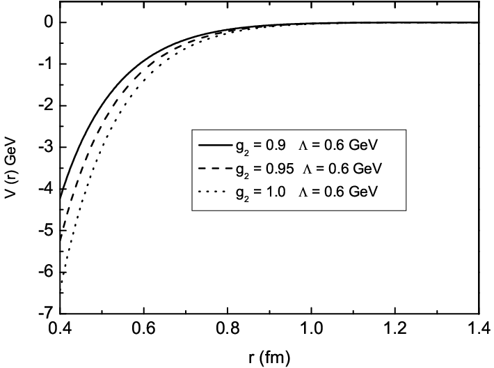
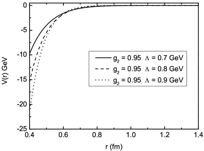
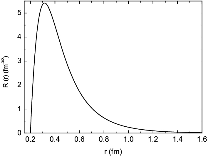
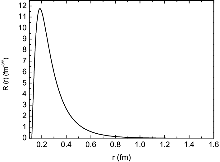
Note that in above asymptotic expressions we keep only those terms up to order 1r5/2\frac{1}{r^{5/2}}, and more singular terms are not taken into accounted in this work. The dependence of potential with various parameters are shown in Figure 3. The results indicate that the potential approaches to zero quickly in long range in every case, while in short range the potential diverges very much with different parameters, as expected. As a result, the binding energy heavily depends on input parameters, the coupling constants and cutoff. One can read from the figure that in the small coupling situation, the potential becomes too narrow and shallow to bind two heavy baryons. Table 2 presents the binding energies of Λc\Lambda_{c}-Λ¯c\bar{\Lambda}_{c} and Σc\Sigma_{c}-Σ¯c\bar{\Sigma}_{c} systems with different inputs. Schematically, the radial wave functions for the ground state of Λc\Lambda_{c}-Λ¯c\bar{\Lambda}_{c} system with Gaussian and monopole form factors are shown in Figure 4 respectively, while the wave functions for Σc\Sigma_{c}-Σ¯c\bar{\Sigma}_{c} system exhibit similar curves.

Refer to caption
Refer to caption
Figure 3: The Λc\Lambda_{c}-Λ¯c\bar{\Lambda}_{c} central potential behavior in case of Gaussian form factor versus different parameter choices.
Table 2: Binding energies with different inputs with Gaussian form factor. The left table is for the Λc\Lambda_{c}-Λ¯c\bar{\Lambda}_{c} system, and the right one for Σc\Sigma_{c}-Σ¯c\bar{\Sigma}_{c} system.
|g2||g_{2}| Λ⁡(GeV)\Lambda(\mathrm{GeV}) Binding Baryonium
energy mass
<<0.9 <<0.6 No -
0.9 0.6 -22 MeV 4.550 GeV
0.95 0.6 -77 MeV 4.495 GeV
1.0 0.6 -168 MeV 4.404 GeV
0.95 0.7 -196 MeV 4.376 GeV
0.95 0.8 -227 MeV 4.345 GeV
0.95 0.9 -588 MeV 3.984 GeV
g1g_{1} Λ⁡(GeV)\Lambda(\mathrm{GeV}) Binding Baryonium
energy mass
<1.0<1.0 <0.8<0.8 No -
1.0 0.8 -11 MeV 4.895 GeV
1.05 0.8 -61 MeV 4.845 GeV
1.1 0.8 -145 MeV 4.761 GeV
1.05 0.85 -141 MeV 4.765 GeV
1.05 0.9 -266 MeV 4.640 GeV
1.05 0.95 -438 MeV 4.468 GeV
Refer to caption
Refer to caption
Figure 4: Radial wave function of Λc\Lambda_{c}-Λ¯c\bar{\Lambda}_{c} ground state. The left figure is for case of Gaussian form factor under the condition of |g2|=0.95|g_{2}|=0.95 and Λ=0.8\Lambda=0.8, and the right one is for the case of monopole form factor with |g2|=0.9|g_{2}|=0.9 and Λ=0.95\Lambda=0.95.

3.2 Monopole form factor case

In order to regulate the singularities at the origin in configuration space, usually people employ three types form factors in the literature, i.e. the Gaussian, the monopole, and the dipole form factors [34]. For comparison we also calculate the potential with monopole form factor using the same factorization technique, and the basic Fourier transformation for monopole form factor is presented in Appendix for the sake of convenience. Here, in obtaining the analytic expressions for potentials we also take the measure of expanding the corresponding functions in parameter λ\lambda and keeping only the leading term. Then, what obtained from the box-diagram contribution reads

VC​MB​(r)=\displaystyle V_{CM}^{B}(r)= −\displaystyle- g448​π5/2​fπ4​Δ2​r5/2​(m9/24​e−2​m​r+Λ4​m1/24​e−2​Λ​r)\displaystyle\frac{g_{4}^{4}}{8\pi^{5/2}f_{\pi}^{4}\Delta^{2}r^{5/2}}\left(\frac{m^{9/2}}{4}e^{-2mr}+\frac{\Lambda^{4}m^{1/2}}{4}e^{-2\Lambda r}\right) (59)
+\displaystyle+ g44​Λ5/2​m5/28​2​π5/2​fπ4​m+Λ​Δ12​r5/2​e−(m+Λ)​r.\displaystyle\frac{g_{4}^{4}\Lambda^{5/2}m^{5/2}}{8\sqrt{2}\pi^{5/2}f_{\pi}^{4}\sqrt{m+\Lambda}\Delta_{1}^{2}r^{5/2}}e^{-(m+\Lambda)r}\;.

Contributions from triangle and two-pion loop diagrams are

VC​MT​(r)\displaystyle V_{CM}^{T}(r) =\displaystyle= g42​m7/216​π5/2​fπ4​Δ1​r5/2​e−2​m​r+g42​m​Λ5/216​π5/2​fπ4​Δ1​r5/2​e−2​Λ​r\displaystyle\frac{g_{4}^{2}m^{7/2}}{16\pi^{5/2}f_{\pi}^{4}\Delta_{1}r^{5/2}}e^{-2mr}+\frac{g_{4}^{2}m\Lambda^{5/2}}{16\pi^{5/2}f_{\pi}^{4}\Delta_{1}r^{5/2}}e^{-2\Lambda r} (60)
−\displaystyle- g42​m5/2​Λ3/24​2​π5/2​fπ4​m+Λ​Δ1​r5/2​e−(m+Λ)​r\displaystyle\frac{g_{4}^{2}m^{5/2}\Lambda^{3/2}}{4\sqrt{2}\pi^{5/2}f_{\pi}^{4}\sqrt{m+\Lambda}\Delta_{1}r^{5/2}}e^{-(m+\Lambda)r}\;

and

VC​ML​(r)=−(Λ2−m2)​m1/232​2​π3/2​fπ4​r3/2​e−(m+Λ)​r+(Λ2−m2)​Λ1/232​2​π3/2​fπ4​r3/2​e−2​Λ​rV_{CM}^{L}(r)=-\frac{(\Lambda^{2}-m^{2})m^{1/2}}{32\sqrt{2}\pi^{3/2}f_{\pi}^{4}r^{3/2}}e^{-(m+\Lambda)r}+\frac{(\Lambda^{2}-m^{2})\Lambda^{1/2}}{32\sqrt{2}\pi^{3/2}f_{\pi}^{4}r^{3/2}}e^{-2\Lambda r}\; (61)

respectively, where superscript BB, TT, and LL stand for box, triangle and 2​π2\pi loop. Note that since there is no heavy baryon intermediate state in the 2​π2\pi loop process, as shown in the right graph of Figure 2, the potential range of it appears different.
Refer to caption
Refer to caption
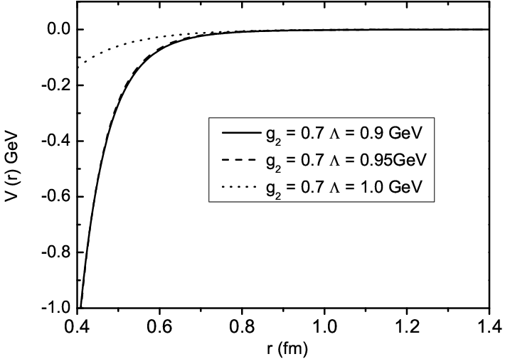
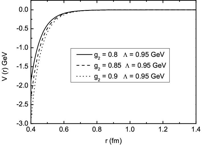
Figure 5: The Λc\Lambda_{c}-Λ¯c\bar{\Lambda}_{c} central potential behavior in case of monopole form factor versus different choices of inputs.

We find that the structure of potential with monopole form factor is much simpler than the Gaussian case. The dependence of potential with various parameters are shown in Fig.5. From the figure one can see that in small coupling case the potential change less, which means the potential tends to be insensitive to the small coupling, and hence the binding energy. Solving the Schrödinger equation we then obtain eigenvalues for different input parameters, given in Table 3. From the table, we notice that the binding energy is sensitive to and changes greatly with the variation of g1g_{1}, |g2||g_{2}| and the cutoff Λ\Lambda, the same as the case with Gaussian form factor. Intuitively, the realistic baryonium can only accommodate small ones of those parameters.

Table 3: Binding energies with different inputs with monopole form factor. The left table is for the Λc\Lambda_{c}-Λ¯c\bar{\Lambda}_{c} system, and the right one for Σc\Sigma_{c}-Σ¯c\bar{\Sigma}_{c} system.
|g2||g_{2}| Λ⁡(GeV)\Lambda(\mathrm{GeV}) Binding Baryonium
energy mass
<<0.7 <<0.9 No -
0.8 0.95 -117 MeV 4.455 GeV
0.85 0.95 -420 MeV 4.152 GeV
0.9 0.95 -521 MeV 4.051 GeV
0.7 0.9 -5 MeV 4.567 GeV
0.7 0.95 -67 MeV 4.505 GeV
0.7 1.0 -252 MeV 4.320 GeV
g1g_{1} Λ⁡(GeV)\Lambda(\mathrm{GeV}) Binding Baryonium
energy mass
<0.9<0.9 <0.9<0.9 No -
0.95 0.95 -438 MeV 4.468 GeV
1.0 0.95 -830 MeV 4.076 GeV
1.05 0.95 -1003 MeV 3.903 GeV
0.9 0.9 -40 MeV 4.866 GeV
0.9 0.95 -153 MeV 4.753 GeV
0.9 1.0 -345 MeV 4.561 GeV

3.3 Ground state of Λb\Lambda_{b}-Λ¯b\bar{\Lambda}_{b} baryonium

Table 4: Binding energies with the change of parameters for Λb\Lambda_{b}-Λ¯b\bar{\Lambda}_{b} system. The left table is for the Gaussian form factor, and the right one for the monopole form factor. Here gbg_{b} corresponds to g2g_{2} in charmed baryonium sector
|gb||g_{b}| Λ⁡(GeV)\Lambda(\mathrm{GeV}) binding Baryonium
energy mass
<<0.7 <<0.7 No No
0.7 0.75 -4 MeV 11.236 GeV
0.8 0.75 -76 MeV 11.164 GeV
0.9 0.75 -294 MeV 10.946 GeV
0.8 0.8 -164 MeV 11.706 GeV
0.8 0.9 -396 MeV 10.844 GeV
0.8 1.0 -622 MeV 10.618 GeV
|gb||g_{b}| Λ⁡(MeV)\Lambda(\mathrm{MeV}) Binding Baryonium
energy mass
<1.0<1.0 <0.8<0.8 No No
1.0 0.8 -11 MeV 11.229 GeV
1.05 0.8 -56 Mev 11.184 GeV
1.1 0.8 -143 MeV 11.097 GeV
1.05 0.8 -103 Mev 11.137 GeV
1.05 0.9 -164 MeV 11.076 GeV
1.05 1.0 -321 MeV 10.919 GeV

We also estimate the ground state of Λb\Lambda_{b}-Λ¯b\bar{\Lambda}_{b} baryonium system with Gaussian and monopole form factors. The result are shown in Table 4, where gbg_{b} corresponds to g2g_{2} in charmed baryonium sector. Note that since the dominant decay mode of Σb\Sigma_{b} is to Λb​π\Lambda_{b}\pi, by which we may constrain the Σb​Λb​π\Sigma_{b}\Lambda_{b}\pi coupling from the experiment result, and this may shed lights on the further investigation on the nature of possible baryonium.

4 Summary and Conclusions

In the framework of heavy baryon chiral perturbation theory we have studied the heavy baryon-baryon interaction, and obtained the interaction potential, the central potential, in the case of two-pion exchange. The Gaussian and monopole types form factors are employed to regularized the loop integrals in the calculation. As a leading order analysis, the tensor potential and higher order contributions in 1MH\frac{1}{M_{H}} expansion are neglected. As expected, we found that the potential is sensitive to the baryon-pion couplings and the energy cutoff Λ\Lambda used in the form factor.

We apply the obtained potential to the Schrödinger equation in attempting to see whether the attraction of two-pion-exchange potential is large enough to constrain two heavy baryons into a baryonium. We find it true for a reasonable choice of cutoff Λ\Lambda and baryon-pion couplings, which is quite different from the conclusion of a recent work in the study of D​D¯D\bar{D} potential through two-pion exchange [35]. Since usually the cutoff Λ\Lambda is taken to be less than the nucleon mass, i.e. about 1 GeV in the literature, in our calculation we adopt a similar value employed in the nucleon-nucleon case. In Ref. [35] authors took a fixed coupling g=0.59g=0.59 and obtained the binding with a large cutoff. While in our calculation for the baryonium system with Gaussian form factor, there will be no binding in case g1<1.0g_{1}<1.0 and Λ<0.8\Lambda<0.8. The increase of coupling constant will lead to an even smaller Λ\Lambda for a given binding energy.

Based on our calculation results it is interesting to note that in case there exists binding in Σc\Sigma_{c}-Σ¯c\bar{\Sigma}_{c} system, with both Gaussian and monopole factors, the coupling g1g_{1} will be much bigger than what conjectured in Ref. [25]. However, for Λc\Lambda_{c}-Λ¯c\bar{\Lambda}_{c} system, to form a bound state the baryon-Goldstone coupling g2g_{2} could be similar in magnitude as what estimated in the literature.

Notice that the potential depends not only on coupling constants and cutoff Λ\Lambda, it also depends on the types of form factors employed. Our calculation indicates that the Gaussian form factor and Monopole form factor are similar in regulating the singularities at origin, and lead to similar results, with only subtle difference, for both Λc\Lambda_{c} and Λb\Lambda_{b} systems. Numerical result tells that the heavy baryon-baryon potentials are more sensitive to the coupling constants in the case of Monopole form factor, but more sensitive to the cutoff Λ\Lambda in the case of Gaussian form factor. From our calculation it is tempting to conjecture that the recently observed states Y⁡(4260)Y(4260) and Y⁡(4360)Y(4360), but not Y⁡(4660)Y(4660) [6], in charm sector could be a Λc\Lambda_{c}-Λ¯c\bar{\Lambda}_{c} bound state with reasonable amount of binding energy, which deserves a further investigation. Our result also tells that the newly observed “exotic” state in bottom sector, the Yb​(10890)Y_{b}(10890) [37], could be treated as the Λb\Lambda_{b}-Λ¯b\bar{\Lambda}_{b} bound state, whereas with an extremely large binding energy.

It is worth emphasizing at this point that although our calculation result favors the existence of heavy baryonium, it is still hard to make a definite conclusion yet, especially with only the leading order two-pion-exchange potential. The potential sensitivity on coupling constants and energy cutoff also looks unusual and asks for further investigation. To be more closer to the truth, one needs to go beyond the leading order of accuracy in 1MH\frac{1}{M_{H}} expansion; one should also investigate the potential while two baryon-like triquark clusters carry colors as proposed in the heavy baryonium model [11, 16]; last, but not least, the unknown and difficult to evaluate annihilation channel effect on the heavy baryonium potential should also be clarified, especially for heavy baryon-antibaryon interaction, which nevertheless could be phenomenologically parameterized so to reproduce known widths of some observed states.

Acknowledgments

This work was supported in part by the National Natural Science Foundation of China(NSFC) and by the CAS Key Projects KJCX2-yw-N29 and H92A0200S2.

Appendix

In this Appendix, we present more detailed formulas and definitions used for the sake of reader’s convenience.

The γ\gamma matrices take the following convention

γ0=(100−1),γi=(0σi−σi0),γ5=(0110).\gamma^{0}=\left(\begin{array}[]{ll}1&0\\ 0&-1\end{array}\right)\;,\;\gamma^{i}=\left(\begin{array}[]{ll}0&\sigma^{i}\\ -\sigma^{i}&0\end{array}\right)\;,\;\gamma_{5}=\left(\begin{array}[]{ll}0&1\\ 1&0\end{array}\right)\;. (62)

And the Dirac spinors for Σc\Sigma_{c} read as

u​(p)=E+MΣ2​MΣ​(χa𝝈⋅pE+MΣ​χa),\displaystyle u(p)=\sqrt{\frac{E+M_{\Sigma}}{2M_{\Sigma}}}\left(\begin{array}[]{l}\chi_{a}\\ \frac{\boldsymbol{\sigma}\cdot\textbf{p}}{E+M_{\Sigma}}\chi_{a}\end{array}\right)\;,

where χa\chi_{a} is two-component Pauli spinor, and

v​(p)=E+MΣ2​MΣ​(𝝈⋅pE+MΣ​ηaηa),\displaystyle v(p)=\sqrt{\frac{E+M_{\Sigma}}{2M_{\Sigma}}}\left(\begin{array}[]{l}\frac{\boldsymbol{\sigma}\cdot\textbf{p}}{E+M_{\Sigma}}\eta_{a}\\ \eta_{a}\end{array}\right)\;,

where ηa=−i​σ2​χa∗\eta_{a}=-i\sigma^{2}\chi_{a}^{*}, and a=1,2a=1,2. Spin-32\frac{3}{2} field for Σ+⁣∗\Sigma^{+*} is described by Rarita-Schwinger spinor uμ​(p,σ)u^{\mu}(p\;,\sigma), which can be constructed by spin-11 vector and spin-12\frac{1}{2} field [36], that is

uμ=E+MΣ+⁣∗2​MΣ+⁣∗​L(1)​(p)νμ​(1𝝈⋅pE+MΣ+⁣∗)​S†ν​ψ​(σ),u^{\mu}=\sqrt{\frac{E+M_{\Sigma^{+*}}}{2M_{\Sigma^{+*}}}}L^{(1)}(p)^{\mu}_{\nu}\left(\begin{array}[]{l}1\\ \frac{\boldsymbol{\sigma}\cdot\textbf{p}}{E+M_{\Sigma^{+*}}}\end{array}\right)S^{\dagger\nu}\psi(\sigma)\;, (69)

where ψ⁡(σ)\psi(\sigma) is four-component Pauli spinor of a spin-32\frac{3}{2} particle, and L(1)​(p)νμL^{(1)}(p)^{\mu}_{\nu} is the boost operator for spin-11 particle,

L(1)​(p)νμ=(EMΣ+⁣∗pjMΣ+⁣∗piMΣ+⁣∗δji−pi​pjMΣ+⁣∗​(E+MΣ+⁣∗)),L^{(1)}(p)^{\mu}_{\nu}=\left(\begin{array}[]{ll}\frac{E}{M_{\Sigma^{+*}}}&\hskip 42.67912pt\frac{p_{j}}{M_{\Sigma^{+*}}}\\ \frac{p_{i}}{M_{\Sigma^{+*}}}&\delta^{i}_{j}-\frac{p^{i}p_{j}}{M_{\Sigma^{+*}}(E+M_{\Sigma^{+*}})}\end{array}\right)\;, (70)

where i,ji,j are indices of the space components of momentum pp. The positive- and negative-energy projection operators for spin-12\frac{1}{2} baryon are

[Λ+​(p)]α​β=∑±suα​(p,s)​u¯β​(p,s)=(p/+MΣc2​MΣc)α​β\displaystyle[\Lambda^{+}(p)]_{\alpha\beta}=\sum_{{\pm}s}u_{\alpha}(p,s)\overline{u}_{\beta}(p,s)=\left(\frac{p\!\!\!/+M_{\Sigma_{c}}}{2M_{\Sigma_{c}}}\right)_{\alpha\beta}\; (71)

and

[Λ−(p)]α​β=−∑±svα(p,s)v¯β(p,s)=(−p/+MΣc2​MΣc)α​β,\displaystyle[\Lambda^{-}(p)]_{\alpha\beta}=-\sum_{{\pm}s}v_{\alpha}(p,s)\overline{v}_{\beta}(p,s)=\left(\frac{-p\!\!\!/+M_{\Sigma_{c}}}{2M_{\Sigma_{c}}}\right)_{\alpha\beta}\;, (72)

respectively.

The positive- and negative-energy projection operators for spin-32\frac{3}{2} baryon are

[Λμ​ν+​(p)]α​β\displaystyle\left[\Lambda^{+}_{\mu\nu}(p)\right]_{\alpha\beta} =∑±suμ,α​(p,s)​u¯ν,β​(p,s)\displaystyle=\sum_{{\pm}s}u_{\mu,\;\alpha}(p,s)\overline{u}_{\nu,\;\beta}(p,s) (73)
=[p/+MΣc∗2​MΣc∗]α​β​(gμ​ν−γμ​γν3−2​pμ​pν3​MΣc∗2+pμ​γν−pν​γμ3​MΣc∗),\displaystyle=[\frac{p\!\!\!/+M_{\Sigma_{c}^{*}}}{2M_{\Sigma_{c}^{*}}}]_{\alpha\beta}\left(g_{\mu\nu}-\frac{\gamma_{\mu}\gamma_{\nu}}{3}-\frac{2p_{\mu}p_{\nu}}{3M_{\Sigma_{c}^{*}}^{2}}+\frac{p_{\mu}\gamma_{\nu}-p_{\nu}\gamma_{\mu}}{3M_{\Sigma_{c}^{*}}}\right)\;,

and

[Λμ​ν−​(p)]α​β\displaystyle\left[\Lambda^{-}_{\mu\nu}(p)\right]_{\alpha\beta} =−∑±svμ,α(p,s)v¯ν,β(p,s)\displaystyle=-\sum_{{\pm}s}v_{\mu,\;\alpha}(p,s)\overline{v}_{\nu,\;\beta}(p,s) (74)
=[−p/+MΣc∗2​MΣc∗]α​β​(gμ​ν−γμ​γν3−2​pμ​pν3​MΣc∗2+pμ​γν−pν​γμ3​MΣc∗),\displaystyle=[\frac{-p\!\!\!/+M_{\Sigma_{c}^{*}}}{2M_{\Sigma_{c}^{*}}}]_{\alpha\beta}\left(g_{\mu\nu}-\frac{\gamma_{\mu}\gamma_{\nu}}{3}-\frac{2p_{\mu}p_{\nu}}{3M_{\Sigma_{c}^{*}}^{2}}+\frac{p_{\mu}\gamma_{\nu}-p_{\nu}\gamma_{\mu}}{3M_{\Sigma_{c}^{*}}}\right)\;,

respectively. Here, μ\mu and ν\nu are Lorentz indices; α\alpha and β\beta are Dirac spinor indices.

The basic Fourier transformation with Gaussian form factor reads

I2​(m,r)\displaystyle I_{2}(m,\;r) =\displaystyle= ∫−∞∞d3​k(2​π)3​ei​kre−k2/Λ2k2+m2\displaystyle\int_{-\infty}^{\infty}\frac{d^{3}\textbf{k}}{(2\pi)^{3}}\frac{e^{i\textbf{kr}}e^{-\textbf{k}^{2}/\Lambda^{2}}}{\textbf{k}^{2}+m^{2}} (75)
=\displaystyle= 18​π​r​em2/Λ2​[e−m​r​e​r​f​c​(−Λ​r2+mΛ)−em​r​e​r​f​c​(Λ​r2+mΛ)],\displaystyle\frac{1}{8\pi r}e^{m^{2}/\Lambda^{2}}\left[e^{-mr}erfc\left(-\frac{\Lambda r}{2}+\frac{m}{\Lambda}\right)-e^{mr}erfc\left(\frac{\Lambda r}{2}+\frac{m}{\Lambda}\right)\right]\;,

and hence

F(λ,r)=∫d3​k(2​π)3ei​kre−k2/Λ2k2+m2+λ2=I2(m2+λ2,r)e−λ2/Λ2.\displaystyle F(\lambda,\;r)=\int\frac{d^{3}\textbf{k}}{(2\pi)^{3}}\frac{e^{i\textbf{kr}}e^{-\textbf{k}^{2}/\Lambda^{2}}}{\textbf{k}^{2}+m^{2}+\lambda^{2}}=I_{2}(\sqrt{m^{2}+\lambda^{2}},\;r)e^{-\lambda^{2}/\Lambda^{2}}\;. (76)

e​r​f​c​(x)erfc(x) is complementary error function, which is defined as

e​r​f​c​(x)=2π​∫x∞e−t2​𝑑t.erfc(x)=\frac{2}{\sqrt{\pi}}\int_{x}^{\infty}e^{-t^{2}}dt\;. (77)

The factorization in double Fourier transformation goes like

H11\displaystyle H_{11} =\displaystyle= ∫∫⁡d3​k1​d3​k2(2​π)6​ei​k1​r1​ei​k2​r2​f​(k12)​f​(k22)ω1​ω2​(ω1+a)​(ω2+a)​(ω1+ω2)\displaystyle\int\int\frac{d^{3}\textbf{k}_{1}d^{3}\textbf{k}_{2}}{(2\pi)^{6}}\frac{e^{i\textbf{k}_{1}\textbf{r}_{1}}e^{i\textbf{k}_{2}\textbf{r}_{2}}f(\textbf{k}_{1}^{2})f(\textbf{k}_{2}^{2})}{\omega_{1}\omega_{2}(\omega_{1}+a)(\omega_{2}+a)(\omega_{1}+\omega_{2})} (78)
=\displaystyle= ∫∫d3​k1​d3​k2(2​π)61a2[2π∫0∞ei​k1​r1​ei​k2​r2​f​(k12)​f​(k22)​d​λ(ω12+λ2)​(ω22+λ2)\displaystyle\int\int\frac{d^{3}\textbf{k}_{1}d^{3}\textbf{k}_{2}}{(2\pi)^{6}}\frac{1}{a^{2}}[\frac{2}{\pi}\int_{0}^{\infty}\frac{e^{i\textbf{k}_{1}\textbf{r}_{1}}e^{i\textbf{k}_{2}\textbf{r}_{2}}f(\textbf{k}_{1}^{2})f(\textbf{k}_{2}^{2})d\lambda}{(\omega_{1}^{2}+\lambda^{2})(\omega_{2}^{2}+\lambda^{2})}
−\displaystyle- 2π∫0∞ei​k1​r1​ei​k2​r2​f​(k12)​f​(k22)​λ2​d​λ(a2+λ2)​(ω12+λ2)​(ω22+λ2)]−1aG11(λ,r1)G11(λ,r2)\displaystyle\frac{2}{\pi}\int_{0}^{\infty}\frac{e^{i\textbf{k}_{1}\textbf{r}_{1}}e^{i\textbf{k}_{2}\textbf{r}_{2}}f(\textbf{k}_{1}^{2})f(\textbf{k}_{2}^{2})\lambda^{2}d\lambda}{(a^{2}+\lambda^{2})(\omega_{1}^{2}+\lambda^{2})(\omega_{2}^{2}+\lambda^{2})}]-\frac{1}{a}G_{11}(\lambda,\;r_{1})G_{11}(\lambda,\;r_{2})
=\displaystyle= 2π​∫0∞d​λa2+λ2​F​(λ,r1)​F​(λ,r2)−1a​G11​(λ,r1)​G11​(λ,r2).\displaystyle\frac{2}{\pi}\int_{0}^{\infty}\frac{d\lambda}{a^{2}+\lambda^{2}}F(\lambda,\;r_{1})F(\lambda,\;r_{2})-\frac{1}{a}G_{11}(\lambda,\;r_{1})G_{11}(\lambda,\;r_{2})\;. (79)

Here,

G11\displaystyle G_{11} =\displaystyle= ∫d3​k1(2​π)3​ei​k1​re−k12/Λ2ω1​(ω1+a)=∫d3​k1(2​π)3​2​aπ​∫0∞ei​k1​re−k12/Λ2dλ(a2+λ2)​(ω12+λ2)\displaystyle\int\frac{d^{3}\textbf{k}_{1}}{(2\pi)^{3}}\frac{e^{i\textbf{k}_{1}\textbf{r}}e^{-\textbf{k}_{1}^{2}/\Lambda^{2}}}{\omega_{1}(\omega_{1}+a)}=\int\frac{d^{3}\textbf{k}_{1}}{(2\pi)^{3}}\frac{2a}{\pi}\int_{0}^{\infty}\frac{e^{i\textbf{k}_{1}\textbf{r}}e^{-\textbf{k}_{1}^{2}/\Lambda^{2}}d\lambda}{(a^{2}+\lambda^{2})(\omega_{1}^{2}+\lambda^{2})} (80)
=\displaystyle= 2​aπ​∫0∞d​λ(a2+λ2)​F​(λ,r),\displaystyle\frac{2a}{\pi}\int_{0}^{\infty}\frac{d\lambda}{(a^{2}+\lambda^{2})}F(\lambda,\;r)\;,

and for simplicity we define ω1=k12+m2\omega_{1}=\sqrt{\textbf{k}_{1}^{2}+m^{2}} and ω2=k22+m2\omega_{2}=\sqrt{\textbf{k}_{2}^{2}+m^{2}}  .

In the case of the monopole form factor, i.e. f⁡(k2)=Λ2−m2Λ2+k2f(\textbf{k}^{2})=\frac{\Lambda^{2}-m^{2}}{\Lambda^{2}+\textbf{k}^{2}}, the corresponding function to F⁡(λ,r)F(\lambda,\;r) reads

R⁡(λ,r)\displaystyle R(\lambda,\;r) =\displaystyle= ∫d3​k(2​π)3​ei​krk2+m2+λ2​Λ2−m2Λ2+k2+λ2\displaystyle\int\frac{d^{3}\textbf{k}}{(2\pi)^{3}}\frac{e^{i\textbf{kr}}}{\textbf{k}^{2}+m^{2}+\lambda^{2}}\frac{\Lambda^{2}-m^{2}}{\Lambda^{2}+\textbf{k}^{2}+\lambda^{2}} (81)
=\displaystyle= 14​π​r​(e−r​m2+λ2−e−r​Λ2+λ2).\displaystyle\frac{1}{4\pi r}\left(e^{-r\sqrt{m^{2}+\lambda^{2}}}-e^{-r\sqrt{\Lambda^{2}+\lambda^{2}}}\right)\;.

Operator O1​(k1,k2)O_{1}(\textbf{k}_{1},\;\textbf{k}_{2}) contains two parts. The first part of O1​(k1,k2)O_{1}(\textbf{k}_{1},\;\textbf{k}_{2}) while acting on functions in configuration space goes like

O1​(k1,k2)​F​(λ,r1)​F​(λ,r2)\displaystyle O_{1}(\textbf{k}_{1},\;\textbf{k}_{2})F(\lambda,\;r_{1})F(\lambda,\;r_{2}) =\displaystyle= (k1⋅k2)2​F​(λ,r1)​F​(λ,r2)\displaystyle(\textbf{k}_{1}\cdot\textbf{k}_{2})^{2}F(\lambda,\;r_{1})F(\lambda,\;r_{2}) (82)
=\displaystyle= (∇1​i∇1​j)​F​(λ,r1)​(∇2​i∇2​j)​F​(λ,r2)\displaystyle(\nabla_{1i}\nabla_{1j})F(\lambda,\;r_{1})(\nabla_{2i}\nabla_{2j})F(\lambda,\;r_{2})
=\displaystyle= 2r2​F′​(λ,r)​F′​(λ,r)+F′′​(λ,r)​F′′​(λ,r),\displaystyle\frac{2}{r^{2}}F^{\prime}(\lambda,\;r)F^{\prime}(\lambda,\;r)+F^{\prime\prime}(\lambda,\;r)F^{\prime\prime}(\lambda,\;r)\;,

where

∇i∇j=(δi​j−xi​xjr2)​(1r​dd​r)+xi​xjr2​(d2d​r2),\nabla_{i}\nabla_{j}=\left(\delta_{ij}-\frac{x_{i}x_{j}}{r^{2}}\right)\left(\frac{1}{r}\frac{d}{dr}\right)+\frac{x_{i}x_{j}}{r^{2}}\left(\frac{d^{2}}{dr^{2}}\right)\;, (83)

and the limit r2→r1=rr_{2}\rightarrow r_{1}=r is taken. The second part of O2​(k1,k2)O_{2}(\textbf{k}_{1},\;\textbf{k}_{2}) while acting on functions in configuration space goes like

O2​(k1,k2)​F​(λ,r1)​F​(λ,r2)\displaystyle O_{2}(\textbf{k}_{1},\;\textbf{k}_{2})F(\lambda,\;r_{1})F(\lambda,\;r_{2}) =\displaystyle= (𝝈1⋅k1×k2)​(𝝈2⋅k1×k2)​F​(λ,r1)​F​(λ,r2)\displaystyle(\boldsymbol{\sigma}_{1}\cdot\textbf{k}_{1}\times\textbf{k}_{2})(\boldsymbol{\sigma}_{2}\cdot\textbf{k}_{1}\times\textbf{k}_{2})F(\lambda,\;r_{1})F(\lambda,\;r_{2}) (84)
=\displaystyle= σ1​i​σ2​j​εi​k​l​εj​m​n​(∇1​k∇1​m)​F​(λ,r1)​(∇2​l∇2​n)​F​(λ,r2)\displaystyle\sigma_{1i}\sigma_{2j}\varepsilon_{ikl}\varepsilon_{jmn}(\nabla_{1k}\nabla_{1m})F(\lambda,\;r_{1})(\nabla_{2l}\nabla_{2n})F(\lambda,\;r_{2})
=\displaystyle= σ1​i​σ2​j​(δi​j​δk​m​δl​n+δi​m​δk​n​δl​j+δi​n​δl​m​δk​jCLOSE\displaystyle\sigma_{1i}\sigma_{2j}(\delta_{ij}\delta_{km}\delta_{ln}+\delta_{im}\delta_{kn}\delta_{lj}+\delta_{in}\delta_{lm}\delta_{kj}
−δl​jδk​mδi​n−δl​mδk​nδi​j−δl​nδi​mδk​j)×\displaystyle-\delta_{lj}\delta_{km}\delta_{in}-\delta_{lm}\delta_{kn}\delta_{ij}-\delta_{ln}\delta_{im}\delta_{kj})\times
(∇1​k∇1​m)​F​(λ,r1)​(∇2​l∇2​n)​F​(λ,r2)\displaystyle(\nabla_{1k}\nabla_{1m})F(\lambda,\;r_{1})(\nabla_{2l}\nabla_{2n})F(\lambda,\;r_{2})
=\displaystyle= 23​[1r2​F′​(λ,r)​F′​(λ,r)+2r​F′​(λ,r)​F′′​(λ,r)]​(𝝈1⋅𝝈2)\displaystyle\frac{2}{3}\left[\frac{1}{r^{2}}F^{\prime}(\lambda,\;r)F^{\prime}(\lambda,\;r)+\frac{2}{r}F^{\prime}(\lambda,\;r)F^{\prime\prime}(\lambda,\;r)\right](\boldsymbol{\sigma}_{1}\cdot\boldsymbol{\sigma}_{2})
+23​(F′​(λ,r)r−F′′​(λ,r))​1r​F′​(λ,r)​S12,\displaystyle+\frac{2}{3}\left(\frac{F^{\prime}(\lambda,\;r)}{r}-F^{\prime\prime}(\lambda,\;r)\right)\frac{1}{r}F^{\prime}(\lambda,\;r)S_{12}\;,

where 𝝈1⋅𝝈2\boldsymbol{\sigma}_{1}\cdot\boldsymbol{\sigma}_{2} gives spin-spin potential and S12=3​(𝝈1⋅r)​(𝝈2⋅r)r2−𝝈1⋅𝝈2S_{12}=\frac{3(\boldsymbol{\sigma}_{1}\cdot\textbf{r})(\boldsymbol{\sigma}_{2}\cdot\textbf{r})}{r^{2}}-\boldsymbol{\sigma}_{1}\cdot\boldsymbol{\sigma}_{2} gives the tensor potential.

References

  • [1] Wolfgang Lucha, Franz F. Schöberl, and Dieter Gromes, Phys. Rept. 200, 127 (1991).
  • [2] C. Quigg and Jonathan L. Rosner, Phys. Rept. 56, 167 (1979).
  • [3] V.A. Novikov, L.B. Okun, M.A. Shifman, A.I. Vainshtein, M.B. Voloshin and V.I. Zakharov, Phys. Rept. 41, 1 (1978).
  • [4] S.K.Choi et al. (Belle Collaboration), Phys. Rev. Lett. 91,262001 (2003).
  • [5] B. Aubert et al. (BarBar Collaboration), Phys, Rev D 77,111101 (2008).
  • [6] B. Aubert et al. (BarBar Collaboration), Phys, Rev Lett 98, 212001 (2007); X. L. Wang et al Belle Collaboration), Phys. Rev. Lett. 99, 142002 (2007); S. K. Choi et al. (Belle Collaboration), Phys. Rev. Lett. 100, 142001 (2008); R. Mizuk et al. (Belle Collaboration), Phys. Rev. D80, 031104 (2009).
  • [7] S. L. Zhu, Phys. Lett. B 625, 212 (2005); E. Kou and O. Pene, Phys. Lett. B 631, 164 (2005); F. E. Close and P. R. Page, Phys. Lett. B 628, 215 (2005); X. Q. Luo and Y. Liu, Phys. Rev. D 74, 034502 (2006); S. L. Zhu, Nucl. Phys. A 805, 221c (2008); S. L. Zhu, Int. J. Mod. Phys. E 17, 283 (2008).
  • [8] X. Liu, X.Q. Zeng, and X.Q. Li, Phys. Rev. D 72, 054023 (2005).
  • [9] F.J. Llanes-Estrada, Phys. Rev. D 72, 031503 (2005).
  • [10] C.-Z. Yuan, P. Wang, and X.H. Mo, Phys. Lett. B 634, 399 (2006).
  • [11] C.-F. Qiao, Phys. Lett. B 639, 263 (2006).
  • [12] G.-J. Ding, Phys. Rev. D 79, 014001 (2009).
  • [13] L. Maiani, V. Riquer, F. Piccinini, and A. D. Polosa, Phys. Rev. D 72, 031502(R) (2005).
  • [14] G.-J. Ding, J.-J. Zhu, and M.-L. Yan, Phys. Rev. D 77, 014033 (2008).
  • [15] B.-Q. Li and K.-T. Chao, Phys. Rev. D 79, 094004 (2009).
  • [16] C.-F. Qiao, J. Phys. G: Nucl. Part. Phys. 35, 075008 (2008).
  • [17] D.V. Bugg, J. Phys. G: Nucl. Part. Phys. 36, 075002 (2009).
  • [18] F.-K. Guo, C. Hanhart, and U.-G. Meiß{\ss}ner, Phys. Lett. B 665, 26 (2008).
  • [19] Z.-G. Wang and X.-H. Zhang, arXiv:0905.3784 [hep-ph].
  • [20] A.M. Badalian, B.L.G. Bakker, and I.V. Danilkin, Phys. Atom. Nucl. 72, 638 (2009).
  • [21] R.M. Albuquerque and M. Nielsen, Nucl. Phys. A 815, 53 (2009).
  • [22] D. Ebert, R.N. Faustov, and V.O. Galkin, Eur. Phys. J. C 58, 399 (2008).
  • [23] N. Brambilla, et al. Heavy quarkonium: progress, puzzles, and opportunities, Eur. Phys. J. C 71, 1534 (2011), arXiv:hep-ph/1010.5827.
  • [24] N. Drenska, et al. New Hadronic Spectroscopy, Riv. Nuovo Cim. 033, 633 (2010), arXiv:hep-ph/1006.2741.
  • [25] Tung-Mow Yan, Y.C. Lin and Hoi-Lai Yu, Phys. Rev D46, 1148 (1992); Hai-Yang Cheng, Tung-Mow Yan et al. Phys. Rev D47, 1030 (1993).
  • [26] A. Manohar and H. Georgi, Nucl. Phys. B 234, 189 (1984).
  • [27] Mark B. Wise, Phys. Rev. D 45, R2188 (1992)
  • [28] Th.A. Rijken and V.G.J. Stoks, Phys. Rev. C46, 73 (1992); Th.A. Rijken and V.G.J. Stoks, Phys. Rev. C46, 102 (1992);
  • [29] Th.A. Rijken, Ann. Phys. 208, 253 (1991).
  • [30] D. Arndt, S.R. Beane and M.J. Savage, Nucl. Phys. A726 339, (2003); S.R. Beane and M.J. Savage, Phys. Lett. B 556, 142 (2003).
  • [31] http://users.ugent.be/ṽledoux/ .
  • [32] K. Nakamura, et al.(Particle Date Group), J. Phys. G: Nucl. Part. Phys. 37, 1 (2010).
  • [33] Th.A. Rijken and V.G. Stoks, Phys. Rev. C54, 2869 (1996).
  • [34] V.G.J. Stoks, R. A. M. Klomp, C. P. F. Terheggen and J. J. de Swart, Phys. Rev. C49, 2950 (1994).
  • [35] Qing Xu, Gang Liu and Hong-Ying Jin, eprint, arXiv:hep-ph/1012.5949.
  • [36] Th.A. Rijken and V.G. Stoks, Phys. Rev. C46, 102 (1992).
  • [37] K.F. Chen, et al., [Belle Collaboration], Phys. Rev. Lett. 100, 112001 (2008).