The collapse transition of randomly branched polymers – renormalized field theory

Usually, one models RBPs by means of so-called lattice animals which are nothing but clusters of connected sites on a regular lattice. One considers as the primary quantity the number $\mathcal{A}(N,l,c)$ of all different configurations (up to translations) of a single cluster (animal) which is a collection of $N$ sites, connected by $b\geq N-1$ bonds, $l$ cycles of the bonds, and $c$ contacts (nearest-neighbor pairs of non-bonded sites). The number of occupied bonds is then given by $b=l+N-1$. There is no need for introducing a separate number $s$ of nearest-neighbor pairs of occupied and non-occupied sites. This number is given by the relation $\mathcal{N}N=2b+2c+s$, where $\mathcal{N}$ is the lattice coordination number, which is equal to $2d$ on a simple hypercubic lattice. The weighted animal number

represents a general partition sum for the system. If one sets $z_{cy}$ to zero, the sum only includes tree configurations. It is well known that this partition function, also known as the generating function of lattice animals, can be obtained from the asymmetric $(n+1)$-state Potts model in the limit $n\rightarrow 0$ [1, 3, 15], and it is this connection, that stands behind the seminal earlier results on RBPs, cf. Sec. I.

Typically, one considers the partition sum for large animals: $N\gg 1$. The phase diagram in this limit in terms of the fugacities $z_{cy}$ and $z_{co}$ is shown in Fig. 1. The special curve $z_{cy}=(z_{co}-1)z_{co}$, parametrized by a bond-probability $p$ as $z_{cy}=p/(1-p)^{2}$, $z_{co}=1/(1-p)$ defines a bond-percolation model with the percolation probability $p=p_{c}$ depending on the specific type of the lattice. In general, if $N\gg 1$, there is a swollen phase for small fugacities, and a compact phase separated by the collapse transition line $z_{co}(z_{cy})$ which consists of two parts separated by the percolation point as a higher order critical point. Whereas in the swollen phase $\mathcal{A}_{N}(z_{cy},z_{co})\sim\kappa_{sw}(z_{cy},z_{co})^{N}N^{-\dot{\theta}}$ with universal $\dot{\theta}$ and non-universal $\kappa_{sw}(z_{cy},z_{co})$, one finds at least for the left part of the transition line the scaling law

with non-universal $\kappa(z_{cy})$, and universal $\theta$ in general different from $\dot{\theta}$ [8]. The percolation point as a separating point on the transition line with higher order critical behavior has a $\theta_{perc}$ which is in general different from $\theta$ and $\dot{\theta}$. Only in mean-field theory (Landau approximation) these exponents are equal: $\theta=\dot{\theta}=\theta_{perc}=5/2$.

Other fundamental quantities are given by correlations of sites on the cluster. The correlation function may be defined by

where $\mathcal{A}(N,l,c;\mathbf{r},\mathbf{r}^{\prime})$ is the total number of clusters with $N$ sites, $l$ loops, and $c$ contacts, containing the lattice sites $\mathbf{r}$ and $\mathbf{r}^{\prime}$. Of course it is

The radius of gyration $R_{N}$ is then defined by

For $N\gg 1$, it shows also an universal scaling law

The fractal dimension $d_{f}=1/\nu_{A}$ is different at the transition line from its value in the swollen phase and at the separating percolation point. However, in mean-field theory it has the uniform value $d_{f}=4$. Of course, in the compact phase, the fractal dimension is always equal to the lattice dimension $d$.

The model that we are about to develop is in the spirit of Landau’s ideas for modeling second-order phase transitions, i.e., it is a mesoscopic model that focuses on general principles unifying processes belonging to the same universality class and is therefore necessarily phenomenological [28]. To set the stage, however, we find it worthwhile to discuss in some detail a specific model belonging to the RBP universality class, viz. a generalization of the GEP. The reaction-diffusion equations defining this process will nurture our intuition and will help us to establish our ideas.

The following generalization of the GEP is a variant of a process that we have introduced for the description of tricritical isotropic percolation [23]. We denote by $X(\mathbf{r})$ an agent, i.e., an infected individual, at site $\mathbf{r}$. An agent can infect a neighboring site $\mathbf{r+\delta}$ via the percolation step

This fundamental reaction gives rise to spreading and branching of the epidemic. The agents can spontaneously become immune (or decay) and produce spam as a marker of the agent through the reactions

where $Z(\mathbf{r})$ denotes an immune individual or spam at site $\mathbf{r}$. In the language of forest fires, the $Z(\mathbf{r})$ are also referred to as debris. It is the debris left behind by the epidemic that forms the clusters which serve us as prototypes for RBPs. Their self-avoidance or excluded volume interaction is modelled with help of the reaction

where $k=1,2,\cdots$, which dampens the epidemic. A mechanism for the RBPs to compactify is introduced into the process through the reaction

which simulates an effective attraction of the agents by the debris.

Having these reactions, one possible way to proceed would be to reformulate the corresponding master-equation in terms of bosonic creation and annihilation operators and then to produce a field theoretic action from these operators via coherent state path integrals [30]. However, we prefer to extract directly the mesoscopic Langevin equations that incorporate the universal features of the above reactions, namely the percolation of agents, their spontaneous decay, their suppression and possible effective attraction by the debris, and the possible existence of vacua without agents as absorbing states of the system.

The primary density-fields describing our generalized GEP are the field of agents $n(\mathbf{r},t)$ and the field of the inactive debris $m(\mathbf{r},t)=\lambda\int_{-\infty}^{t}dt^{\prime}\,n(\mathbf{r},t^{\prime})$ which ultimately forms the polymer cluster. A non-Markovian Langevin equation describing such a process, and represents therefore the universality class, is given by

Here, the parameter $r$ tunes the ”distance” to the percolation threshold. Below this threshold, i.e., in the absorbing phase, $r$ is positive. Throughout this paper, we will assume that the system is deep in the absorbing phase. In this case, a typical final cluster generated from an additional source $q\delta(\mathbf{r})\delta(t)$ of agents adding such a source is equivalent to specifying an initial condition for the process) consists of $N=\langle\int d^{d}r\,m(\mathbf{r},\infty)\rangle\approx q/r$ debris-particles, and has a mean diameter $1/\sqrt{r}$. However, we are interested in the large non-typical clusters, the rare events of the stochastic process, with $N\gg q/r$. We know from percolation theory [24] that these clusters belong to the universality class of lattice animals. Hence, they are the same in a statistical sense as randomly branched polymers as far as their universal properties go. The gradient-term proportional to $c$ describes the attractive influence of the debris on the agents if $c$ is negative (as a negative contribution to $g^{\prime}$ does). At this point other forms of gradient-terms like $m\nabla^{2}n$ and $n\nabla^{2}m$ are conceivable. However al long as we include any one of these gradient terms into our theory, an omission of the other gradient terms has no effect on the final results, and we choose to work with the term proportional to $c$ only for simplicity. For usual percolation problems (ordinary or tricritical), these gradient terms are irrelevant. As long as $g^{\prime}>0$, the second order term $f^{\prime}m^{2}$ is irrelevant near the transition point and the process models ordinary percolation near $r=0$ [31] or non-typical very large clusters, the swollen RBPs, for $r>0$. We permit both signs of $g^{\prime}$ (negative values of $g^{\prime}$ correspond to an attraction of the agents by the debris, see above). Hence, our model allows for a tricritical instability (tricritical percolation near $r=0$ [23] or the collapse transition of the RBPs for $r>0$). Consequently we need the second order term $f^{\prime}>0$ (which represents the self-avoidance property) to limit the density to finite values. Physically it originates from the suppression of agents by the debris. The Gaussian noise-source $\zeta(\mathbf{r},t)$ has correlations

The process is assumed to be locally absorbing, and thus all terms in the noise-correlation function contain at least one power of $n$. The first part of the noise correlation takes into account that the agents decay spontaneously, and thus $g>0$. The non-Markovian term proportional to $f$ simulates the anticorrelating or, respectively, correlating (from attraction) behavior of the noise in regions where debris has already been produced with $f$ being negative if the attraction effects are overwhelming.

Two points are worth mentioning at this stage: (i) For the Langevin-equation with the local noise to be meaningful mathematically, an appropriate cut-off procedure of long wavelengths has to be used. (ii) The stochastic process (11) with $c=r=g^{\prime}=f^{\prime}=g=0$ but $f>0$ belongs to the universality class of self-avoiding random walks (SAW), and generates therefore the statistics of linear polymers [32].

To proceed towards a field theoretic model, the Langevin equations are now transformed into a stochastic response functional in the Ito-sense [33, 34, 35, 28]

With this functional, we now have a vantage point for the calculation of statistical quantities via path-integrals with the exponential weight $exp(-\mathcal{J})$. When a source-term $(\tilde{h},\tilde{n})$ is added, where $\tilde{h}(\mathbf{r},t)=\tilde{h}_{0}(\mathbf{r},t)=q\delta(\mathbf{r})\delta(t)$ and $(..,..)$ denotes an integral of a product of two fields over space and time, this functional describes, in particular, the statistics of clusters of debris generated by the stochastic process (11) from a source of $q$ agents at the point $\mathbf{r}=0$ at time zero. Denoting by $\operatorname*{Tr}\bigl[\ldots\bigr]$ the functional integration over the fields, we generally have

if $h$ or $\tilde{h}$ are zero. The first property follows from causality whereas the second one originates from the absorptive properties of the process. Note that the role of causality and adsorptivity can be interchanged via the duality transformation $m(\mathbf{r},t)\longleftrightarrow-\tilde{n}(\mathbf{r},-t)$ [31, 36, 28].

Averaging an observable $\mathcal{O}[n]$ over final clusters of debris (the RBPs) of a given mass $N$ generated from a source $\tilde{h}(\mathbf{r},t)=q\delta(\mathbf{r})\delta(t)$ of agents at the origin $\mathbf{r}=0$ at time $t=0$ leads to the quantity [31, 28, 36]

where

is the probability distribution for finding a cluster of mass $N$.

is the total mass of the debris. The field $m_{\infty}(\mathbf{r})=m(\mathbf{r},t=\infty)$ describes the distribution of the debris after the epidemic has become extinct. Since the probability distribution should be proportional to the number of different configurations, we expect by virtue of universality arguments the following proportionality between the probability distribution $\mathcal{P}(N)$ and the lattice animal number $\mathcal{A}_{N}$ for asymptotically large $N$:

where $\kappa_{0}$ is an effective coordination number of the underlying lattice. The fugacities in $\mathcal{A}_{N}(z_{cy},z_{co})$ are then considered as analytical functions of the different parameters in the response functional $\mathcal{J}$ or vice versa. The factor $N^{-1}$ arises in Eq. (18) because the generated clusters are rooted at the source at the point $\mathbf{r}=0$, and each site of a given lattice animal may be the root of given cluster. Hence, we expect a scaling

with an universal scaling exponent $\theta$ but non-universal $p_{0}$.

In actual calculations, the delta function appearing in averages like in Eq. (16) is hard to handle. This problem can be simplified by using Laplace-transformed observables like, e.g., the Laplace transformation of $\mathcal{P}(N)$, which are functions of a variable conjugate to $N$, say $z$,

and applying inverse Laplace transformation (where all the singularities of the integrand lie to the left of the integration path) in the end. Note that the relationship between $\mathcal{P}(N)$ and $\mathcal{A}_{N}$ signals the existence of a singularity $\sim(z-z_{c})^{\theta-2}$ of the integrand in Eq. (20) at some critical value $z_{c}$. The switch to Laplace-transformed observables can be done in a pragmatic way by augmenting the original $\mathcal{J}$ with a term $z\mathcal{M}$ and then working with the new response functional

Denoting averages with respect to the new functional by $\langle\ldots\rangle_{z}$, and defining

for small $q$, we get by using Jordans lemma that the asymptotic behavior for large $N$ is given by

where the last row gives the asymptotics for large $N$ and small $q$. Here, $z_{c}$ is the first singularity of $\Phi(z)$, which as we will show is a branch point on the negative real axis, and the contour of the path integral is deformed into a path above and below the branch cut beginning at the singularity. $\operatorname*{Disc}\Phi$ denotes the discontinuity of the function $\Phi$ at the branch cut. The non-universal factor $q\mathrm{e}^{z_{c}N+q\Phi(z_{c})}$ depending exponentially on $N$ is common to all averages defined by Eq. (15) and therefore cancels from all mean values $\langle\mathcal{O}\rangle_{N}$.

Before we assent to the heights of field theory (or decent to its depths, if the reader prefers, we first apply a mean-field approximation to our theory, i.e., we solve the functional integrals with the weight $\exp(-\mathcal{J}_{z})$ using a saddle-point approximation. The linear term in $\mathcal{J}_{z}$ that is proportional to the Laplace-variable $z$ leads to a non-zero saddle-point value of the field $\tilde{n}$:

Therefore, shifting this field, $\tilde{n}\rightarrow\tilde{n}+\Phi$, so that

the harmonic (Gaussian) part of $\mathcal{J}_{z}$ becomes

Here, we have implied that the saddlepoint-value of $m_{\infty}$ is zero, i.e., we have assume that $\rho=(g^{\prime}+f\Phi)\Phi$ is positive. If $\rho=0$, which is the case near the tricritical instability of our stochastic process, a phase transition to a positive value of $\langle m_{\infty}\rangle$ sets in. Whether or not this transition is the anticipated collapse transition deserves some further scrutiny. A shift

(which does not change the condition (25)) changes $\Phi(g^{\prime}+f\Phi)$ to $\Phi(g^{\prime}+f\Phi)+\alpha\tau$, where $\tau=r-g\Phi$. The special value $\alpha=-c\Phi/2$ eliminates the gradient-term $\sim(\nabla m_{\infty})^{2}$ and hence $\rho=0$ signals the collapse only if $\tau$ goes to zero which is indeed the critical value corresponding to large clusters with $N\gg 1$. This can be seen from the saddlepoint condition $h=z+r\Phi-g\Phi^{2}/2=0$ that leads to

Thus, the meanfield-solution shows a branch-point singularity at $z_{c}=-r^{2}/2g$, and $\tau(z)=\sqrt{r^{2}+2gz}$ becomes zero at this singularity.

Until now, we have kept the gradient term proportional to $c$ in our theory. The discussion in the last paragraph revealed that this term is redundant in the sense of field theory as it can be eliminated via the shift transformation (27). Hence, we will formally set $c=0$ unless noted otherwise.

Next, let us calculate $\mathcal{P}(N)$ from Eq. (23). Inserting $\Phi(z)$ from Eq. (28), we easily obtain the probability density of branched polymers with size $N$ in mean-field approximation,

The maximum of this distribution is found at $N=N_{0}=q/r$. For $N\gg q/r$, the distribution drops down exponentially. However, this is the region of rare events of our stochastic process where the large branched polymers are found. Hence, small $q$ means effectively $q\ll rN$, and $q=1$ is ‘small’ in this region. Combining Eqs. (2) and (18), we obtain the asymptotic result

and the well-known mean-field animal exponent $\theta=5/2$ common to the swollen phase, the percolation point, as well as the collapse transition-line.

Now, we calculate the monomer distribution (the distribution of the debris-particles) of a single large cluster rooted at the point $\mathbf{r}=0$. We recall from our remarks above that such a root is represented field theoretically by an insertion of the field $\tilde{n}(0,0)$. According to Eq. (15), the monomer distribution is given by the inverse Laplace transformation of the correlation function calculated with the harmonic response functional (26):

It follows that

This function can be written in terms of generalized hypergeometric series ${}_{0}F_{2}$, however, we prefer the integral representation shown in Eq. (32). Easily, we verify the sum rule

The radius of gyration $R_{N}$ can be calculated straightforwardly from its definition,

Hence, the gyration exponent is $\nu_{A}=1/4$ as anticipated. The integral representation (32) yields the asymptotic forms of the monomer distribution for $\left|\mathbf{r}\right|\ll R_{N}$

and

if $\left|\mathbf{r}\right|\gg R_{N}$. We see that the monomer-distribution in the fractal interior of the cluster has a fractal dimension $d_{f}=4$ independent of $N$. The distribution in the outer region drops down exponentially in $\left|\mathbf{r}\right|$, however, with an exponent $4/3=1/(1-\nu_{A})$. Besides the exponential factor, the distribution decreases algebraically with an exponent $(d-2)/3=(d/2-d\nu_{A}+2-\theta)/(1-\nu_{A})$. We will show later on that these scaling relations comprising the independent critical exponents $\theta$ and $\nu_{A}$ hold generally and are not restricted to the mean-field approximation.

Another interesting quantity is the correlation of two roots. Evidently, two roots can either belong to one cluster or they can belong to two separate clusters. Their correlation function is of some value in polymer physics because it determines the second virial coefficient of the equation of state of a dilute solution of branched polymers. The connected part of this correlation function, i.e., the cumulant, is given by

Inverse Laplace-transformation leads to

in the region $\left|\mathbf{r}\right|\gg R_{N}$, where $N$ should be understood here as the total number of monomers. Since the correlation of roots on the same cluster goes down proportionally to the density of monomers on one single cluster, the increasing behavior of the fraction

results mainly from the interaction of two separate clusters. They are repelling one another if $\rho$ is positive, and attracting one another for negative $\rho$. The sharp difference between repelling and attracting is a clear signature of the collapse transition located at $\rho=0$. Note that a contribution to $\rho$ proportional to $\tau$ as discussed above leads only to a change of the pivotal factor $\rho N^{1/2}$ of order $1$ since $\tau(z)$ converts to a term $\sim N^{-1/2}$ through the inverse Laplace-transformation.

Now, we return to our response functional to refine it into a form that suits us best for our actual field theoretic analysis. As discussed above, the gradient term proportional to $c$ is redundant. To eliminate this term, we apply to the field $\tilde{n}$ the shift and mixing transformation

where $\Phi$ is a free parameter at this stage. Defining in consistency with our mean-field considerations above $\tau=r-g\Phi$, $\rho=(g^{\prime}+f\Phi)\Phi-c\Phi\tau$, $h=z+r\Phi-g\Phi^{2}/2$, the stochastic functional $\mathcal{J}_{z}$ (21) takes the form

Here, we could have set $\tau$ equal to zero by exploiting that $\Phi$ is a free parameter. Instead of doing so, we rather keep $\tau$ in our theory as a small free parameter. We will see later on that keeping $\tau$ comes in handy for renormalization purposes. In Eq. (41), we have eliminated couplings that are of more than third order in the fields because they are irrelevant. We do not write down in detail the relatively uninteresting relations between the new third-order coupling constants and the old ones. Note that $\mathcal{J}_{z}$ contains two similar couplings: $g_{2}^{\prime}\tilde{n}nm$ and $g_{1}\tilde{n}nm_{\infty}$. Whereas the first coupling respects causal ordering, which means that $\tilde{n}$ is separated by an infinitesimal positive time-element from the $nm$-part resulting from the Ito-calculus [35], the second one respects causality only between $\tilde{n}$ and $n$. In contrast to the $m$-part, the $m_{\infty}$-part contains all the $n$ with times that lie in the past and in the future of $\tilde{n}$. This property is the heritage of the time-delocalized noise term. Even if we had disregarded the noise term proportional to $f$ in Eq. (12) initially, the $\tilde{n}nm_{\infty}$-coupling would be generated by coarse graining, and hence it must be ultimatively incorporated into the theory to yield a renormalizable theory.

The relevance of the different terms in $\mathcal{J}_{z}$ follows from their dimensions with respect to an inverse length scale $\mu$ such that time scales as $\mu^{-2}$. Fundamentally, one has to decide which parameters are the critical control-parameters going to zero in mean-field theory. As we have seen, at the collapse transition these are $\tau\sim\rho\sim\mu^{2}$, and $h\sim\mu^{(d+2)/2}.$ The dimensions of the fields are then given by $\tilde{n}\sim m\sim\mu^{(d-2)/2}$, and $n\sim\mu^{(d+2)/2}$. It follows that all the coupling constant $g_{0}$, $g_{1}$, $g_{2}$, and $g_{2}^{\prime}$ have the same dimension $\mu^{(6-d)/2}$. Note that $\tilde{n}$ is tied always to at least one factor of $n$ as a result of absorptivity of the process. Hence, we have retained all the couplings that are relevant for $d\leq 6$ spatial dimensions, and the model is renormalizable below the upper critical dimension $d_{c}=6$ of the collapse transition. The situation is different if $\rho$ is a finite positive quantity, that is in the swollen phase. Then $\rho$ can be absorbed into the fields by a scale transformation which amounts to formally setting $\rho=2$. The field dimensions then become $m\sim\mu^{d/2}$, $n\sim\mu^{(d+4)/2}$, and $\tilde{n}\sim\mu^{(d-4)/2}$. It follows that $h\sim\mu^{d/2}$, $g_{0}\sim\mu^{-d/2}$, $g_{1}\sim\mu^{(4-d)/2}$, $g_{2}^{\prime}\sim\mu^{(2-d)/2}$, and $g_{2}\sim\mu^{(8-d)/2}$. Hence, in the swollen phase only $g_{2}=g$ is relevant, now below $8$ spatial dimensions. The other couplings can be safely removed.

In the following, we focus on the static properties of the generated clusters after the epidemic has become extinct. Here, we are interested only in time-independent static expectation values of the form $\langle\prod_{i}m_{\infty}(\mathbf{r}_{i})\prod_{j}\tilde{n}(\mathbf{r}_{j},0)\rangle$. Thus, we take the quasi-static limit [31, 28, 23, 18], see Appendix A, by setting $\tilde{n}(\mathbf{r},t)\rightarrow\tilde{n}_{0}(\mathbf{r})=:\varphi(\mathbf{r})$ in the dynamic response functional $\mathcal{J}_{z}$. We rename $m_{\infty}(\mathbf{r})=:\tilde{\varphi}(\mathbf{r})$ and get

where we have denoted the original time-delocalisation of the $\tilde{n}nm_{\infty}$-term by a separating dot in $\tilde{\varphi}{\varphi\cdot}\tilde{\varphi}$. Using the quasistatic limit, one has to be careful to account for the former causal ordering of fields in the diagrammatic perturbation expansion. This means that one has to rule out diagrams with closed propagator-loops. But note that only the $\tilde{\varphi}{\varphi}$-part of the $\tilde{\varphi}{\varphi\cdot}\tilde{\varphi}$-term can contribute to such a closed loop.

Of course these additional rules make the perturbation expansion very clumsy in higher loop-order calculations. Fortunately there exists an elegant way to overcome these difficulties associated with the additional rules by introducing so-called ghost fields whose sole purpose is to generate additional diagrams that cancel any diagrams with non-causal propagator-loops. Such a procedure does not change the physical content of the theory but simplifies calculations and makes it easier to find higher symmetries. To one-loop order, non-causal loops are easily cancelled by a corresponding loop of contrary sign. The ghost fields for producing such loops that come to mind first are a pair of fermionic fields. Note, however, that $D$ independent similar bosons can also create a loop with a negative sign in the limit $D\rightarrow-2$, see Fig. 2.

To be more specific, the ghost fields that we use are $D$ independent bosonic fields $(\psi_{1},\ldots,\psi_{D})$, in the limit $D\rightarrow-2$ which is taken at the end of the calculation. These ghosts are incorporated into our theory be adding the term

to the integrand of $\mathcal{J}_{z}$ (42). Note that this term arises formally if one replaces each causal ordered $\tilde{n}n$-pair in $\mathcal{J}_{z}$ by the sum over $\psi_{k}\psi_{k}/2$-pairs. Here comes a new symmetry into play: the additional term (43) is trivially invariant under any permutation of the $D$ ghost fields $\psi_{k}$, i.e., we have symmetry under the permutation (or symmetric) group $S_{D}$. However, since in general $\sum_{k=1}^{D}\psi_{k}\neq 0$, this representation is reducible. Hence, it is more useful to introduce new ghost fields $(\chi_{1},\ldots,\chi_{D+1})$ with constraint $\sum_{\alpha=1}^{D+1}\chi_{\alpha}=0$, and $\sum_{k=1}^{D}\psi_{k}^{2}=\sum_{\alpha=1}^{D+1}\chi_{\alpha}^{2}=:\chi^{2}$. This is easily achieved by using $D+1$ Potts–spin-vectors $\vec{e}^{(\alpha)}=(e_{k}^{(\alpha)})$ directed to the corners of a $D$-dimensional simplex. The spin-vectors have the usual properties: $\sum_{\alpha=1}^{D+1}e_{k}^{(\alpha)}=0$, $\sum_{\alpha=1}^{D+1}e_{i}^{(\alpha)}e_{k}^{(\alpha)}=\delta_{ik}$, $\sum_{k=1}^{D}e_{k}^{(\alpha)}e_{k}^{(\beta)}=\delta_{\alpha\beta}-1/(D+1)$. Hence, the relation between the old and the new ghosts are given by $\chi_{\alpha}=\sum_{k=1}^{D}e_{k}^{(\alpha)}\psi_{k}$. Now, we have symmetry under the permutation group $S_{D+1}$ of permutations of the $(D+1)$ ghost fields $\chi_{\alpha}$, and this representation is irreducible.

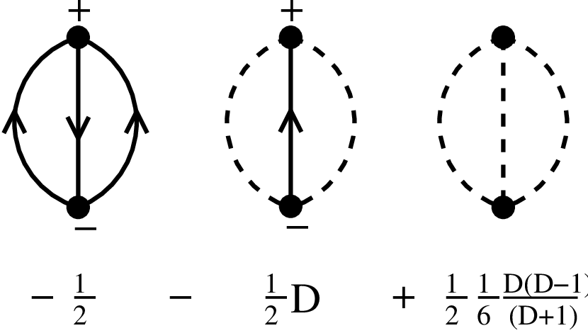
Inspection shows that the ghosts also work in multi-loop diagrams provided that the non-causal loops are separated from each other in these diagrams [18]. However, as long as $g_{2}^{\prime}$ is not zero (note that $g_{2}$ is always greater than zero because otherwise only diagrams without loops are generated), non-separated non-causal loops arise, see the first diagram in Fig. 3. The cancellation requires a permutation-symmetric irreducible interaction $\chi^{3}=\sum_{\alpha=1}^{D+1}\chi_{\alpha}^{3}$ of the $(D+1)$ ghosts, see the third diagram in Fig. 3. Using these new ghosts, the quasi static Hamiltonian becomes

Perturbation theory with this Hamiltonian is no longer burdened with additional rules. It will serve as the vantage point of our RG calculations. As it stands, it is general enough to capture both the swollen phase and the collapse transition. As we have shown in mean field theory, the collapse transition corresponds to vanishing $\tau$, $\rho$, and $h$. Swollen RBPs correspond to vanishing $\tau$ and $h$, but positive and finite $\rho$.

The Hamiltonian (44) is form-invariant under three transformations of the fields. Therefore, three parameters of the Hamiltonian are redundant. One of these transformations, the mixing $\varphi\rightarrow\varphi+\kappa\tilde{\varphi}$, $\tilde{\varphi}\rightarrow\tilde{\varphi}$, we have already used to eliminate the gradient term $(\nabla\tilde{\varphi})^{2}$. The second of these transformations, the rescaling $\varphi\rightarrow\lambda\varphi$, $\tilde{\varphi}\rightarrow\lambda^{-1}\tilde{\varphi}$ can be used either to identify coupling-constants $g_{2}^{\prime}=g_{2}$, or to transform $g_{2}$ to one and use only scaling-invariant quantities. Via the third transformation, the shift $\varphi\rightarrow\varphi+\gamma$, $\tilde{\varphi}\rightarrow\tilde{\varphi}$, either $\tau$ or $\rho$ can be transformed away. At this point, a word of caution is in order. Using these transformations to eliminate parameters from the field theoretic functional, one is well advised to make sure that non of the parameters $\kappa$, $\lambda$, or $\gamma$ featured in the transformations is singular. Otherwise, parameters eliminated from the unrenormalized theory will have to re-emerge in the renormalization procedure. This is no problem per se, but it is a fact that can be easily overlooked, and if so, will lead to ill-defined renormalization schemes.

Before moving on to our actual RG calculation, we find it worthwhile to comment on the renormalizability of $\mathcal{H}$. Simple power counting shows that the ghosts have the same dimensionality as the fields $\tilde{\varphi}$ and ${\varphi}$, namely $\chi_{\alpha}\sim\mu^{(d-2)/2}$. For the swollen phase, the coupling constants $g_{0}$, $g_{1}$, and $g_{2}^{\prime}$ are irrelevant and hence can and should be set equal to zero. Then one can easily ascertain that the remaining $\mathcal{H}$ contains all the relevant terms generated under renormalization, and hence $\mathcal{H}$ is renormalizable as far as the swollen phase is concerned. For the collapse transition, the situation is more intricate. Simple inspection by means of power counting lends credence to the renormalizability of $\mathcal{H}$. However, one has to be more careful here, because the way the various $g$’s appear in multiple places, i.e., a given $g$ may appear as a factor of different monomials of the fields, viz. in couplings amongst the ghost, in couplings amongst the primary fields $\varphi$ and $\tilde{\varphi}$, and in couplings of the primary fields and the ghosts. Does this spoil renormalizability? The answer is clearly no because we know for certain that $\mathcal{H}$ is renormalizable by virtue of its equivalence in the quasi-static limit to the renormalizable dynamic functional $\mathcal{J}_{z}$ which is renormalizable. Hence, there must exist some hidden symmetry that masks the renormalizability of $\mathcal{H}$. Once revealed, this underlying symmetry will provide for relations between different vertex-functions. We will show shortly that this is the symmetric group $S_{D+2}$ (not only the permutation symmetry $S_{D+1}$ of the $D+1$ ghosts alone) of the permutation of $(D+2)$ field combinations. First, however, we will look briefly at a $1$-loop calculation that underpins and exemplifies the considerations just presented.

The elements of our diagrammatic perturbation expansion, the propagators, the correlators, and the vertices, are listed in Fig. (4) and Fig. (5), respectively. For the time being, we focus here just on the decorations of Feynman diagrams, i.e., the combinations of coupling-constants and symmetry-factors of the diagrams without the integrations over loop-momenta. We list the relevant $1$-loop diagrams, writing them in a form that makes evident the cancellations in the limit $D\rightarrow-2$. For the tadpole-diagrams, Fig. (6), we find

References

- [1] T.C. Lubensky and J. Isaacson, Phys. Rev. Lett. 41, 829 (1978), Phys. Rev. Lett. 42, 410(E) (1978), Phys. Rev. A 20, 2130 (1979).
- [2] J. Isaacson and T.C. Lubensky, J. Physique Lett. 41, L469 (1980).
- [3] A.B. Harris and T.C. Lubensky, Phys. Rev. B 23, 3591 (1981), Phys. Rev. B 224, 2656 (1981).
- [4] G. Parisi and N. Sourlas, Phys. Rev. Lett. 46, 871 (1981).
- [5] Y. Shapir, Phys. Rev. A 28, 1893 (1983).
- [6] P. G. deGennes, Biopolymers 6, 715 (1968).
- [7] R. Bundschuh and T. Hwa, Phys. Rev. Lett. 83, 1479 (1999); Phys. Rev. E 65, 031903 (2003); Phys. Rev. Lett. 100, 148101 (2008).
- [8] H.-P. Hsu and P. Grassberger, J. Stat. Mech., P06003 (2005).
- [9] H.-P. Hsu, W. Nadler, and P. Grassberger, J. Phys. A: Math. Gen. 38, 775 (2005).
- [10] B. Derrida and H.J. Herrmann, J. Physique 44, 1365 (1983).
- [11] M. Henkel and F. Seno, Phys. Rev. E 53, 3662 (1996).
- [12] F. Seno and C. Vanderzande, J. Phys. A: Math. Gen. 27, 5813, 7937 (1994).
- [13] S. Flesia, D.S. Gaunt, C.E. Soteros and S.G. Whittington, J. Phys. A: Math. Gen. 25, L1169 (1992); 27, 5831 (1994).
- [14] E.J. Janse van Rensburg et al., J. Phys. A: Math. Gen. 30, 8035 (1997); 32, 1567 (1999); 33, 3653 (2000).
- [15] A. Coniglio, J. Phys. A: Math. Gen. 16, L187 (1983).
- [16] F. Family and A. Coniglio, J. Phys. A: Math. Gen. 13, L403 (1980).
- [17] H.K. Janssen and A. Lyssy, J. Phys. A: Math. Gen. 25, L679 (1992); Europhys. Lett. 29, 25 (1995).
- [18] H.K. Janssen and A. Lyssy, Phys. Rev. E 50, 3784 (1994).
- [19] J. Cardy, J. Phys. A: Math. Gen. 34, L665 (2001).
- [20] D.C. Brydges and J.Z. Imbrie, Ann. Math. 158, 1019 (2003); J. Stat. Phys. 110, 503 (2003).
- [21] For a very clear pedagogically presentation of the work of Brydges and Imry see J. Cardy, arXiv:cond-mat/0302495v3.
- [22] H.K. Janssen and O. Stenull, Europhys. Lett. 90, 46003 (2010).
- [23] H.K. Janssen, M. Műller, and O. Stenull, Phys. Rev. E 70, 026114 (2004).
- [24] D. Stauffer and A. Aharony, Introduction to Percolation Theory (Taylor and Francis, London, 1994).
- [25] C. Becchi, A. Rouet, and R. Stora, Comm. Math. Phys. 52, 55 (1975).
- [26] D.J. Amit, Field Theory, the Renormalization Group, and Critical Phenomena (World Scientific, Singapore, 1984).
- [27] J. Zinn-Justin, Quantum Field Theory and Critical Phenomena (Clarendon, Oxford, fourth edition 2002).
- [28] H.K. Janssen and U.C. Täuber, Ann. Phys. 315, 147 (2005).
- [29] H.K. Janssen, F. Wevelsiep, and O. Stenull, Phys. Rev. E 80, 041809 (2009).
- [30] For a recent review on the coherent path-integral approach see U.C. Täuber, M. Howard, and B.P. Vollmayr-Lee, J. Phys. A 38, R79 (2005).
- [31] H.K. Janssen, Z. Phys. 58, 311 (1985).
- [32] For a review, see e.g., L. Schäfer, Excluded Volume Effects in Polymer Solutions (Springer-Verlag, Berlin, 1999).
- [33] H.K. Janssen, Z. Phys. B 23, 377 (1976); R. Bausch, H.K. Janssen, and H. Wagner, Z. Phys. B 24, 113 (1976).
- [34] C. DeDominicis, J. Physique C 37, 247 (1976); C. DeDominicis and L. Peliti, Phys. Rev. B 18, 353 (1978).
- [35] H.K. Janssen, in: Dynamical Critical Phenomena and Related Topics, Lecture Notes in Physics, Vol. 104, ed. C.P. Enz (Springer, Heidelberg, 1979); H.K. Janssen, in: From Phase Transition to Chaos, ed. G. Györgyi, I. Kondor, L. Sasvári, T. Tél (World Scientific, Singapore, 1992).
- [36] H.K. Janssen, J. Phys. C: Cond. Mat. 17, S1973 (2005).
- [37] H.K. Janssen and O. Stenull, in preparation.
- [38] H.K. Janssen and O. Stenull, in preparation.
- [39] J. des Cloiseaux, Phys. Rev. A 10, 1665 (1974).
- [40] M.E. Fisher, J.Chem. Phys. 44, 616 (1966).
- [41] D. McKenzie and M. Moore, J. Phys. A: Math. Gen. 4, L82 (1971).