Semiclassical solitons in strongly correlated systems of ultracold bosonic atoms in optical lattices
Abstract
We investigate theoretically soliton excitations and dynamics of their formation in strongly correlated systems of ultracold bosonic atoms in two and three dimensional optical lattices. We derive equations of nonlinear hydrodynamics in the regime of strong interactions and incommensurate fillings, when atoms can be treated as hard core bosons. When parameters change in one direction only we obtain Korteweg-de Vries type equation away from half-filling and modified KdV equation at half-filling. We apply this general analysis to a problem of the decay of the density step. We consider stability of one dimensional solutions to transverse fluctuations. Our results are also relevant for understanding nonequilibrium dynamics of lattice spin models.
pacs
03.75.Be, 32.80.Pj, 42.50.VkI Introduction
Solitons are conspicuous manifestations of nonlinear interactions in a variety of physical systems (see e.g. [73, 51]). Originally introduced in hydrodynamics of classical fluids, they were later observed in a variety of other systems, including plasma physics, nonlinear optics, magnetism, dynamics of molecular systems. It is currently understood that formation of oscillatory zones and localized solitonic solutions is a common feature of many non-linear systems and does not depend on the exact integrability of the model. However the character of solitons is different for each system and understanding their properties remains a fundamental problem in physics and mathematics.
In this paper we investigate theoretically the nature of solitons and dynamics of their formation in strongly correlated systems of ultracold bosonic atoms in optical lattices [42, 12, 61, 13]. Recently questions of far from equilibrium many-body dynamics took central stage in both theoretical and experimental study of ultracold atoms. What makes such systems particularly well suited for exploring quantum dynamics is their good isolation from the environment. Their characteristic energies and frequencies are of the order of kiloHertz, which is extremely convenient for experimental studies. It is also important that a wide array of experimental tools that allow to control system parameters in time and prepare far from equilibrium initial states have been developed. Recent experiments addressed such question as dynamics of fermions in optical lattices [88, 84], observation of superexchange interactions using spin dynamics [91], thermalization and relaxation in one-dimensional systems [50, 37, 34], motion of impurity particles [53], dynamics and adiabaticity in crossing classical and quantum phase transitions [78, 81]. Another important recent achievement is development of experimental tools for the in-situ imaging of individual atoms in optical lattices [70, 74, 27, 45, 5, 87] and low dimensional condensates [36, 102]. This technique allows unprecedented level of characterization of many-body states and should lead to deeper understanding of their out of equilibrium dynamics. One example is recent analysis of Bakr et al [5] of the dynamics of defect creation in crossing from the SF to Mott state in two dimensional optical lattices.
We start our analysis by deriving hydrodynamical approach to describe quantum dynamics of the lattice bosons. Hydrodynamical description has been applied to quantum many-body systems previously, including superfluids [48], superconductors [31], quantum Hall systems [93], and magnets[35]. The focus of most earlier analysis was on understanding collective modes and universal features of linear response functions, which only required understanding linear hydrodynamics. When non-linear effects have been discussed for superfluid systems, it was primarily done for systems in the continuum with the the full Galilean symmetry. Our goal will be to include both nonlinearities and dispersion, since the competition of the two determines the nature and dynamics of solitons.
Solitons in systems of ultracold atoms have been discussed previously in the regimes where semiclassical Gross-Pitaevskii equation can be applied either in uniform systems [15, 19, 49, 76, 16] or systems with optical lattices [22, 90, 2, 3, 95, 43, 47]. In this paper we will be interested in the regime of very strong interactions between atoms, the so-called hard core bosons regime [82, 85]. In this case dynamics of atoms in a lattice can be described using anisotropic Heisenberg model[82]. We demonstrate that in this regime the character of soliton excitations is very different and depends on both the filling factor and parameters of the Heisenberg model. Numerical analysis of solitons in Bose systems in optical lattices in the vicinity of the SF/Mott transition has been done recently by Krutitsky et al. [55]. Our results can also be applied to study nonequilibrium spin dynamics of two component Bose mixtures in the Mott insulating regime[21, 52] and lattice spin systems in solid state physics.
II Model
II.1 From lattice bosons to spin Hamiltonian
Microscopic model describing ultracold bosonic atoms in an optical lattice is given by the Bose-Hubbard model[42, 13]
| (1) |
Here is a creation operator for bosons on site , is the number of atoms on site . We do not include the chemical potential term because in this paper we study dynamics and the operator of the total number of particles commutes with the Hamiltonian. It is sufficient to impose a certain number of particles at the initial time and then the total number of particles should not change during evolution. When there is inhomogeneous external potential we also need to add
| (2) |
To keep the model more general we include nearest neighbor interactions
| (3) |
Such non-local interaction are relevant for atoms in higher Bloch bands[83] and polar molecules in optical lattices[56]. We consider a regime when the local repulsion is large and the density of particles is incommensurate with the lattice. In this case strong number fluctuations are suppressed even in the superfluid state and we can limit the Hilbert space to only two possible occupation numbers and per site. It is convenient to represent these states as spin states. State corresponds to , and state corresponds to . In this limit Hamiltonian (3) is equivalent to the anisotropic Heisenberg model
| (4) |
Here are Pauli matrices, , and .
II.2 Semiclassical equations of motion for lattice bosons
In this section we discuss how one can obtain semiclassical description of dynamics of (4) using either variational Gutzwiller wavefunctions or linearized equations of motion, which in this case are equivalent to lattice Landau-Lifshitz equations. To simplify the derivation we assume that parameters of the system change in one direction only. We emphasize that our focus is on two and three dimensional systems. Restriction to having variations of parameters in only one direction is, firstly, for notational simplicity (extension to higher dimensions is straightforward) and, secondly, because we will be concerned with problems where initial state has been prepared to have parameters changing along one of the coordinates. We discuss effects of fluctuations in transverse directions in subsequent sections.
Strictly one dimensional systems are special and mean-field approaches do not apply to them even in equilibrium. However special analytical approaches are available for one dimensional systems, including fermionization and Bethe ansatz[25, 29, 89]. Also powerful numerical methods based on DMRG [86] and Matrix Product States[17] allow to study dynamics of one dimensional systems in great details. On the other hand, nonequilibrium dynamics of higher dimensional systems remains largely unexplored. This is the main motivation for the current paper. Interestingly, recent work by Lancaster and Mitra [57] showed that semiclassical analysis of Landau-Lifshitz equations for one dimensional spin chains give results consistent with exact calculations. Hence our results may also be relevant for one dimensional spin chains.
To obtain semiclassical dynamics we consider time-dependent variational wavefunctions
| (5) |
Expectation values of the original boson operators are
| (6) |
To project Schrodinger equation into wavefunction (5) we define the Lagrangian [41, 40]
and write equations of motion
| (7) |
Here corresponds to both and . We find
| (8) |
The first equation is effectively the Josephson relation: time derivative of the phase is equal to the chemical potential which depends on the values of and . The second equation is charge conservation.
One can give an alternative physical interpretation to equations (8). We write equations of motion for spin operators
| (9) |
And we have analogous equations for . To obtain semiclassical dynamics we replace operators by their expectation values
| (10) |
These are familiar Landau-Lifshitz equations. If we use wavefunction (5) to calculate and , we recognize that Landau-Lifshitz equations are equivalent to (8).
Dynamics of the Bose-Hubbard model has been studied using Gutzwiller variational wavefunctions in [101, 18, 68, 39]. In [4, 77] this approach was used to describe current decay in the strongly interacting regime of bosons. Theoretical predictions were in quantitative agreement with subsequent experimental results by Mun et al[67].
III Semiclassical dynamics in the continuum limit
III.1 Long wavelength expansion
It is convenient to introduce slow variables in space, , and time, , where is the lattice constant. We are looking at dynamics of fluctuations that are slow on the scale of the lattice constant. So is a small parameter in which we will expand. We introduce
| (11) |
and obtain
| (12) |
III.2 Hydrodynamics
If we keep only the lowest order terms in in (12), we obtain the hydrodynamic part of the lagrangian
| (13) |
It is convenient to define
The new variable is proportional to the phase gradient, .
Equations of motion obtained from the lagrangian (13) have a standard hydrodynamic form
| (15) |
III.3 Linearized equations of motion. Stable and unstable regimes.
Let us consider a superfluid state with a uniform density and, possibly, finite phase winding. When , this is a current carrying state with .
Frequencies of linearized excitations are given by the eigenvalues of the matrix
We have for the eigenvalues of
| (19) |
When and is small, both eigenvalues of (III.3) are real (when this is true for all ). This is the hyperbolic regime, which will be the main focus of our paper.
When , eigenvalues of (III.3) appear as a complex conjugate pair. This is the elliptic regime, which corresponds to the unstable state of the system. In this regime small fluctuations of the plane wave type
grow exponentially in time. Existence of this unstable regime is known as the dynamical instability [94, 4]. It was observed experimentally for atoms in optical lattices[23, 67]. Exponential growth of small modulations predicted by equations (15) is only valid for short times. Dynamics of the unstable regime beyond the short time limit can be analyzed using mathematical methods from the theory of elliptic equations. In this paper we only address the stable hyperbolic regime.
When the initial state does not carry a current, i.e. there is no phase winding,
| (20) |
To obtain further insight into the linearized system we set
We can now rewrite equation (15) in terms of variables and , which describe small deviations from the equilibrium state
| (21) |
System (21) gives the following equation for
| (22) |
We find the familiar wave equation, which describes propagation of the initial perturbation with a small amplitude. Equations (21) and (22) show that during the dynamical evolution of the perturbation, the superfluid velocity is of the order of , provided that this is true in the initial state. This is the regime that will be the focus of our paper.
III.4 Nonlinearities and appearance of singularities
We now include nonlinear terms in the analysis of equations of motion. In the simplest case we can define
| (23) |
And from the Lagrangian (13) we obtain equations of motion
Equations (III.4) are written in terms of the Riemann invariants, which separate the system (15) into the left- and right-moving parts. This representation is most convenient in the analysis of Hydrodynamic Type systems. System of equations (III.4) admits two natural reductions or , which describe separate propagation of the left- and right-moving excitations.
When , expressions for Riemann invariants are more cumbersome
The corresponding diagonal system of the equations of motion has a character close to (III.4) in the hyperbolic regime.
Taking in the account that the functions and have the same order in our approach we can write
| (28) |
In the same way
| (29) |
To understand the role of non-linear effects we expand the corresponding equations of motion up to second order terms in deviations from the uniform state. We obtain the following general form of the equations of motion
| (30) |
Equations (30) describe coupled evolution of the right and left moving parts. To get further insight into dynamics we make another simplification. In the problems that we consider the left and right moving parts overlap at short times, but separate after a finite time. The main effects of non-linearities appear at long times. Thus when discussing effects of non-linearities it is sufficient to consider separately the left- and right-moving parts of the solution. So when we discuss the dynamics of we can set and vice versa.
After we make the Galilean transformation for the left and right propagating parts we obtain
| (31) |
| (32) |
Equations (31) and (32) are known as the Hopf equations describing ”simple waves”. Their solutions are given by the implicit formula
The most important feature of these solutions is that they exist only up to a finite time , which depends on the initial conditions. All nontrivial solutions become singular after some finite time. Physically this corresponds to formation of the breaking point, which we show in Fig. 1. This can be understood as a result of regions of different densities moving with different velocities.

Formation of the singularity is not restricted to the truncated equations of motion (30). This is a feature of the general non-linear dynamics of the equations of motion (III.4). Generally system of equations (15) can be reduced to a linear problem using the so-called hodograph transformation. Then solutions of (15) can be described in terms of perturbations moving along the characteristic lines . Characteristics of the nonlinear system depend on the variables and unique solutions of (15) exist only up to a finite time . At later times solution becomes multi-valued. Special solutions of (15) given by relations or describe perturbations moving along one of the characteristic lines. In this case the second variable ( or ) satisfies a nonlinear first order equation, which is (locally) equivalent to the nonlinear Hopf equation.
For times approaching solutions of (31), (32) are close to developing a breaking point and have high gradients. In this regime neglecting higher order gradients in the Lagrangian (12) is no longer justified. In the next section we will see that taking dispersion into account suppresses singularities in the solutions and gives rise to short-period oscillations.
General analysis of how dispersion leads to the formation of oscillatory zones in our system is rather complicated. In the most generic case, one can not use expansion (12) to describe the oscillatory zone formation. The period of oscillations arising for is of the order of , so all higher dispersive corrections are of the same order. Accurate description of the transition from the ”slowly-modulated” to the rapidly modulated regimes can only be done with the use of the original lattice system (8). However, there are certain special cases, in which the use of the continuum model (12) is justified. Fortunately these cases are interesting from the experimental point of view. They will be the subject of our discussion.
IV Nonlinear waves in generic case
IV.1 Connection to Korteweg-de Vries equation
When discussing dispersive terms for and in the equations of motion, it is sufficient to keep them only in the linear order in deviations from the uniform state. Dispersive terms come with additional factors of and are already small. Hence in the Lagrangian (12) dispersive terms need to be considered only up to quadratic terms in or . Modulo total derivatives with respect to we can write
The resulting equations of motion are
| (33) |
Using variables , we obtain
| (34) |
| (35) |
As in our earlier discussion we consider separately the left and right moving parts, i.e. we take either or . After we included effects of dispersion such reductions are no longer exact. However, in cases of interest, interaction between and gives rise only to small rapid oscillations. Such oscillations are expected to be much smaller than the structures that we discuss (see e.g. [54]) and we will neglect them in this paper. We also perform Galilean transformations for the two parts and obtain in the moving coordinate systems
| (36) |
| (37) |
Note that equations (36), (37) transform into each other if we change . Equivalence of the two equations for fixed values of , and represents an evident corollary of the symmetry of the original system.
Depending on the values of parameters , , and , equations (36) and (37) are equivalent to one of the following two equations
| (38) |
| (39) |
after an appropriate rescaling of coordinates and functions . These two equations are equivalent to each other if we admit the inversion , . However, this transformation leads to very different physical interpretation of solutions for a fixed , as we discuss below.11 1 In the next chapter we will also discuss that solutions of (38) and (39) demonstrate different stability properties with respect to two-dimensional modulations.
KdV type equations (38) and (39) allow solitonic solutions, which are long lived nonlinear excitations in the system. The velocity of a soliton is proportional to its amplitude, so larger solitons move faster than the smaller ones. The asymptotic form of an -soliton solution for for equations (38) and (39) can be represented as shown at Fig. 2.

In the Appendix X.1 we briefly review how one can verify the existence of solitonic excitations in the KdV equation using connection to the linear Schroedinger equation. We also point out that in general, solutions of (38) and (39) include not only the soliton part but also ”wave trains”. The soliton part and the ”wave train” parts separate from each other at long times (Fig. 3). The soliton part of the solution remains unchanged for all while the wave - train part ”dissolves” as ([98]). From our point of view, solitons of (38) and (39) represent the most interesting part of the solution and we focus on them in this paper.

IV.2 Discussion of solitonic excitations
Solitons in KdV equations have been studied in detail during the last few decades. In this paper we take previously known mathematical results and discuss their physical implications for our specific system. While we provide a brief summary of the mathematical methods used in analyzing soliton excitations in the Appendix, we refer readers to the books [1, 71, 72] for a more detailed discussion of general mathematical aspects of the KdV equation.
The character of solitonic solutions of KdV type equations (38) and (39) depends on parameters. In particular depending on the ratio of and the density, isolated solitons can appear either as particle-like or hole-like excitations. In this subsection we only provide a summary of the results. More details can be found in the Appendix.
In the discussion below we only consider the case , which corresponds to the density above half-filling . Equations (36) and (37) have a symmetry , . This symmetry originates from the particle-hole symmetry of the initial system, which relates states below and above half-filling (8) : and . In our discussion this symmetry allows to relate solitonic excitations below and above half-filling. For solitons are ”mirror images” of the case. For example, if we find particle-like solitons above half-filling, we should have hole-like solitons below half-filling () for the same values of . Let us represent here also the form of the ”hole-like” and the ”particle-like” solitons in the original variables (see Fig. 4).

We also remind the readers that we only need to consider states that are stable against dynamical modulations, i.e. .
IV.2.1 Solitons for and .
In this case both equations (36), (37) reduce to equation (39) after rescaling the variables and, if necessary, performing the transformation . There should be no solitons when . We are guaranteed to find solitonic excitations when
| (40) |
When the soliton part represents the main part of the solution. So we find particle-like solitons in this situation.
IV.2.2 Solitons for and
Now both equations (36), (37) reduce to equation (38) after rescaling the variables and doing the transformation in equation (37). This equation does not have any solitons when . It has guaranteed solitonic solutions when
| (41) |
In the case with the soliton part represents the main part of the solution. Hence in terms of the original density, we find the hole-type solitons in this case.
IV.2.3 Solitons for and
Both the equations (36), (37) reduce to equation (39) in this case. Thus we find particle-like solitons in terms of the original density.
We can now summarize results of this subsection. When we find that above half-filling there are only particle-like solitonic excitations. When and above half-filling we find that we have either hole-like (closer to half-filling) or particle-like solitons (closer to filling factor one).
IV.3 Self-consistency of the long wavelength expansion
Before concluding this section we would like to verify that our solutions do not take us outside the region of applicability of Lagrangian (12), which was obtained using long wavelength expansion. When we consider dynamics starting from a state with small smooth deviations from a uniform density, approximate Lagrangian (12) can be certainly used at the initial stages of the evolution. However, at final (asymptotic) stages of the evolution, the solution may be sufficiently different from the initial state. Let us consider specifically the soliton part of asymptotic solutions. In soliton solutions both the nonlinear and dispersive parts are important and the interplay of the two gives rise to a stable soliton. One of the important properties of the KdV equation is that the amplitude of solitons is of the same order as initial deviations from the uniform density. Equations (36) - (37) were obtained assuming small deviations of the initial density from the uniform value . These small deviations set the scale for the amplitude of resulting solitons. In solitons there is a direct relation between the amplitude and the width (the width increases as the amplitude goes to zero). Hence in the limit that we discuss, the dispersion part of our soliton solutions should be small, and our approximation of neglecting higher dispersion corrections should be justified even for the final stages of the evolution. For example, when solution can be written as the ”quasiclassical solution”, in which the soliton part represents the main contribution to the solution, higher dispersive and nonlinear terms should have very weak effect on the soliton.
Similar considerations are applicable for the ”wave-train” part of the solutions. However, the ”wave-train” part dissolves in the limit and we expect that it will be more challenging to observe it in experiments.
V Nonlinear waves in special cases
V.1 Half-filling. Solitons of the modified Korteweg-de Vries equation
When the particle density is , the system of hard core bosons has a full particle-hole symmetry. Eigenvalues of the linearized system (21) have the largest possible magnitude
which corresponds to the largest possible velocity of linear waves. In the case of dynamics starting from some initial state, this should provide fastest spatial separation of the left- and right-moving parts of the perturbation. In this case , so corrections to , which are linear in and , vanish and we need to use quadratic terms in the expansion (28). In our discussion below we keep linear terms, in order to accommodate small . Using approximation (29) we can write
From the last two equations we determine how propagation of the left- and right- moving parts, (36)-(37), is modified by the higher order terms. Within the assumptions of spatial separation of the left- and right-moving parts, which we used in the earlier discussion, and using appropriate moving frames of reference we find
| (42) |
| (43) |
In writing the last equations we omitted higher order corrections in . When . equation (42) can be written in the canonical form
| (44) |
after a scaling transformation. Parameter that we introduced here is proportional to the deviation from half-filling, , and we assume it to be small.
Equation (44) is called the modified Korteweg - de Vries (mKdV) equation and represents an integrable system as well as the KdV equation (see [92]). Let us note also that the mKdV equation is connected with the KdV equation by the Miura transformation ([66]) which was the first observation of the integrability properties of the KdV equation itself (see [71]).
There is a wider variety of soliton excitations that one can construct in the mKdV problem. At a fixed value of the chemical potential one can find both particle-like and hole-like solitons moving in the same direction. This should be contrasted to the situation away from half-filling, which we discussed in the previous section, where at a given chemical potential and direction of propagation we had either particle or hole like solitons, but never both simultaneously. For the mKdV case we also find soliton excitations which look like particle on a pedestal (or hole on a pedestal). We provide a detailed discussion of solitons in the mKdV problem and their manifestations for our system in the Appendix.
V.2 Close to integer filling. Nonlinear Schroedinger equation
When the system is close to integer filling . In this case characteristic velocities of the linearized system (21) coincide. Hence we can no longer assume separation of the left- and right-moving parts. Examining system (34)-(35) we find that dispersive corrections also have singularities in variables .
To avoid these difficulties we return to variables , which we used before, and consider the Lagrangian density
| (45) |
in the limit . If we keep only quadratic terms in in the dispersive part of the Lagrangian, we can write the corresponding equations of motion as (in the limit )
| (46) |
If we keep only the lowest order cubic terms in the nonlinear part of (46), we can rewrite this equation for small as
().
It is not difficult to verify that the system above can be written in the form of the defocusing nonlinear Shrödinger equation
| (47) |
for the function
Equation (47) describes an integrable system ([99]), which was solved by V.E. Zakharov and A.B. Shabat by the inverse scattering method. System (47) admits an exact description of the evolution starting from any initial state. However, nonlinear Shrödinger equation does not have soliton solutions in the defocusing case. Defocusing nature of equation (47) demonstrates stable behavior of the system with respect to initial perturbations. In this case asymptotic behavior of solutions of (47) should only include wave-trains which ”dissolve” for ([98]). 22 2 The soliton solutions on the ”pedestal” are also possible for equation (47). We do not consider them here.
V.3 Special filling factor
We now comment on the special point of our system at
| (48) |
for the case . To get equations (38) - (39) from (36) - (37) we need to make scaling transformation
This transformation is singular at the special point (48). As a corollary, the width of solitons (and the period of oscillations in the ”wave-train” part) become small in -space w.r.t. another parameter
Higher dispersive terms become important in this limit and Lagrangian density (12) can no longer be used. As we discussed earlier, dynamics is more complicated near this special point, and one should use original lattice system (8) to discuss dynamics. In general we expect here oscillation zones with rather short period of oscillations.
VI Decay of the density step
We now apply our general arguments to understand dynamical evolution starting from a specific initial state. We assume that at we have a smooth step-like change in the density without any initial current. Experimentally such initial configuration can be created using a smooth step in the external potential that is suddenly removed. This initial state is of the form given by equation (20). It is shown schematically in Fig. 5. In this section we only consider the situation when the system is not close to any special points. Density step decay for systems close to half-filling is discussed in the Appendix.
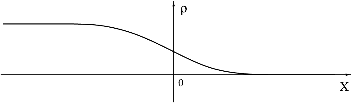

Since we rely on the long wavelength expansion, we assume that function is a slow function of the spatial coordinate.
The main terms in the long wavelength expansion of dynamics are given by the wave equation (21). The wave equation predicts that after a short time the step-like initial state should turn into a two-step solution, with two steps propagating in the opposite directions (see Fig. 6). When the two steps separate from each other, they can be analyzed independently. The left- and right-moving edges of the solution correspond to and . Proceeding to the next order in , we find that they are described by equations (36) and (37) respectively. After rescaling of coordinates and functions and themselves, this dynamics is given either by equation (38) or (39), where the choice depends on the values of , , and .

First of all, we need to understand whether hydrodynamic solutions for and break down and develop a singularity. For and the initial density profile shown in Fig. 5 the steepness of function should increase with time while the steepness of function should decrease with time (see Fig. 7). This follows from simple hydrodynamic analysis following equations (31) and (32). This means that the steepness of solutions , will increase on the left-moving edge of Fig. 6 and decrease on the right-moving edge. (The situation changes to the opposite for the inverse step initial state.) So in this case no dispersive corrections are needed for . Function should remain smooth for all in the hydrodynamic approximation. On the other hand, function develops a breaking point in the hydrodynamic approximation. Thus we need to consider equation (36) taking into account dispersive corrections. As we discussed before dispersive corrections should give rise the oscillation zone, which we expect to grow linearly with time. The form of oscillations should be different for equations (38) and (39) due to different signs of dispersion in these systems (see Fig. 8 - 9).


To understand the oscillation zone that arises following breaking of the hydrodynamic solution we need to analyze dynamics of the KdV equation with step like initial conditions. This problem was addressed by A.V. Gurevich and L.P. Pitaevskii ([32, 33]) using the Whitham theory of slow modulations. We will now summarize their key results pointing out their implications for our system.
Gurevich and Pitaevskii considered a general problem of slowly modulated one-phase solution of the KdV equation. One-phase solution is a periodic running wave solution that provides a generalization of the one-soliton solutions of the KdV equation
One-phase solution depends on three parameters . Functions should be -periodic in , so parameter plays the role of the wave number for nonlinear running waves. Parameter plays the role of the amplitude of the periodic solution, while parameter is the value of averaged over one period (see Fig. 10).

One-phase solutions of KdV can be written in the form
where is the modulus of the Jacobi elliptic function , . The values can be expressed in terms of the parameters in the following way
where and are the elliptic integrals of the first and the second kind respectively.
We can also write
as normalization of function .
The one-soliton solutions of KdV can be considered as the limiting case of the one-phase solutions in the large-period limit . Traditionally the asymptotes , is assumed for the soliton solutions of KdV, so the amplitude parameter remains the one parameter of a one-soliton solution.
In Whitham’s approach parameters become slow functions of and
so that functions , , satisfy a nontrivial system of quasilinear equations in partial derivatives (the so-called Whitham’s system). Whitham’s system describes evolution of initial parameters , , of oscillating solutions, such that development of oscillations can be calculated in this case.
Gurevich and Pitaevskii showed that in the KdV equation with a step like initial conditions, the small oscillation zone, that arises near the breaking point of the hydrodynamic solution, can be described by the self-similar solutions characterized by only one variable, .
In more details, the asymptotic () form of oscillations can be described by the modulated one-phase solutions of KdV with parameters , , of the form
The oscillation zone is located in the interval
in this asymptotic regime.
According to [32] - [33] the amplitude of oscillations becomes zero at the ”trailing edge” of the oscillation zone (the right edge in Fig. 8 and the left edge in Fig. 9). The wave number of nonlinear oscillations becomes zero at the ”leading edge” of the oscillation zone (the left edge in Fig. 8 and the right edge in Fig. 8).
We can see that the ”trailing edge” of oscillation zone can be considered as a source of oscillations with small amplitude, which develop into solitons in the limit . The ”leading edge” of the oscillation zone can be considered as a source of free solitons since we have on this edge and the distance between solitons tends to infinity for .
We point out that it is also possible to analyze the problem above in terms of the ”pure” soliton picture ([59, 60]). Approach used in ([59, 60]) is also a classical part of the soliton theory.
General problem of the decay of different initial configurations in the theory of small-dispersion KdV-equation represents a big branch of the soliton theory. While we do not discuss other problems here, we expect that many of the known mathematical results will be relevant for different experiments with ultracold atoms. We also point out that our methodology for identifying the character of solitons (particle- or hole-like) was based on considering the function , which describes Riemann invariants or . It is more natural to classify solitons based on the density. Relations between and the more physical variables of the density, , and the phase gradient, , are given in equation (29). We find that the density always follows the behavior of . Hence our classification of the hole-type and the particle-type solitons in terms of the density coincides with that given in terms of the function .
Before concluding this section we would like to point out that whether step-like conditions shown in Fig. 5 should be considered as a source of hole-like or particle-like solitons in the solutions , depends on the relation between parameters . In general, we expect that larger values of and suppress the appearance of hole-type solitons and favor solitons of the particle type. On the opposite side, smaller values of and allow solitons of the hole type and suppress solitons of particle type.
VII Two-dimensional effects.
In this section we discuss the role of transverse directions. We consider a question of whether one dimensional profiles, that we discussed so far, are stable against ”weak” modulation in the transverse direction.
For a -dimensional lattice we need to change the long wavelength Lagrangian density (45) to a more general expression
or
in the coordinates .
We separate the hydrodynamic and dispersive parts of the Lagrangian and repeat considerations used in the previous sections. Analysis of the dynamical system is more complicated for and we will not explore all of its richness. We only address a question whether one dimensional solitons that we discussed so far are stable with respect to formation of a two dimensional pattern (see Fig. 11).
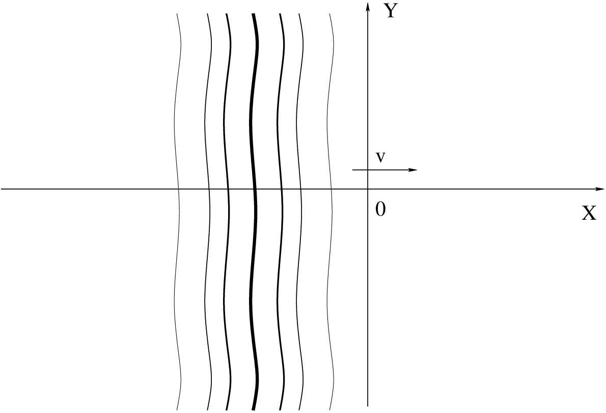
We start with a generic situation corresponding to equation (38) or (39). Since we are going to consider only small modulations of the soliton strings, we can follow the procedure suggested in [44] to get the Kadomtsev - Petviashvili equation for two-dimensional systems.
Firstly we recall that equations (36)-(37) are written in the moving coordinate systems. For the left-moving part of the solution in the laboratory frame of reference we have
| (49) |
In writing the last equation we preserved the restriction
The first term in the right-hand part plays the main role in the evolution of and other terms represent small corrections with respect to the main contribution. According to [44] we only need to calculate corrections to the main term coming from the slow modulation of the solution in the -direction. This procedure gives us stable or unstable variants of the Kadomtsev - Petviashvili equation. The main term in the right-hand part of (49) originates from the linear system (21) of (22) which can be easily written in the two-dimensional form by adding additional derivatives in the -direction. What we need here is correction to the dispersion law which can be written as
for the left-moving part in our situation33 3 We use the expansion of the solutions of linear system in the form .. As a result, the small modulations in the -direction of solutions of (49) can be described by the equation
or
| (50) |
in the moving coordinate system.
Equation (50) is the Kadomtsev - Petviashvili (KP) equation which describes the small transverse modulations of solutions of the KdV equation considered in the two-dimensional case. The stable Kadomtsev - Petviashvili equation corresponds to the same signs of the coefficients for and . In this case the small modulation of a soliton string causes just the weak oscillations along the string and does not produce any instability. The opposite situation with different signs of the coefficients before and corresponds to the unstable situation where the soliton strings are unstable with respect to modulation along the -axis.
We can see then that the stable soliton string in two dimensions arises for the situation of equation (38), i.e.
which corresponds to the small values of and the density in the pattern.
The solutions we considered in the opposite situation
are unstable from the point of view of the two-dimensional modulations.44 4 Let us note here that these conclusions do not require in fact the square two-dimensional lattice and are applicable for any dispersion law , in the main linear approximation.
Let us say now that the analogous considerations can be performed also in the case of equation (44) so the results formulated above can be used also in the limit .
We must certainly say that the Kadomtsev - Petviashvili equation is an integrable system from the point of view of the inverse scattering methods ([20, 100]). The theory of equation (50) is very deep and brought many beautiful ideas in the theory of solitons. Let us just mention here two nice classes of solutions of (50) in the stable and the unstable situation.
1) The most interesting solutions of the Kadomtsev - Petviashvili equation in the stable situation are the two-dimensional -soliton solutions which are described in general by the formula
with some special functions ([80]).
The -solution solutions of the KP equation represent plane interacting waves propagating at some angles with respect to each other. The interaction of the waves results in the phase shifts which can be rather big in the resonant case ([65]).
2) For the unstable variant of the KP equation very interesting rational localized solutions (”lumps”) can arise. The ”lumps” represent localized both in and direction solitons with rational dependence of coordinates. The interaction of solitons does not produce any phase shifts in this situation, so the solitons completely ”forget” about each other after the interaction ([11]).
Let us emphasize here that the relation was assumed everywhere in our considerations above and the properties we consider will be completely changed for the opposite situation . Thus, as we pointed out already, the hydrodynamic approximation (15) reveals an elliptic instability for the small values of () in this situation which corresponds to a modulation instability of long-wave solutions of (8) in this case. In the same way, equation (47) becomes the focusing nonlinear Shrödinger equation in this situation which corresponds to the unstable behavior of the long-wave solutions of (8) either. However, the integrable nature of the focusing nonlinear Shrödinger equation leads to very interesting behavior of solutions also in this case. The most interesting part is the presence of the -soliton solutions for the focusing NLS equation which should be observed for . The corresponding two-dimensional equation for (47) can be written in the form
| (51) |
VIII Concluding remarks
Soliton solutions in quantum systems is a subject of considerable theoretical interest. However, most of the earlier work focused on one dimensional systems, where special analytical tools, such as the Bethe ansatz solution, are available. For example, exact solitonic solutions were considered recently in a different quantum system in a series of papers [8, 9, 10]. Their analysis relied on the quantum inverse scattering methods, which are special to 1d integrable systems. Our analysis in this paper is on constructing semiclassical solitons in two and three dimensional systems.
States described by the wavefunction (5) correspond to collective excitations in the superfluid state. In the superfluid state the U(1) symmetry is spontaneously broken, so the number of particles is not a good quantum number. Solitons which we discuss in this papers are semiclassical collective excitations. They can be thought of as spatially inhomogeneous coherent states representing non-linear excitations of the Hamiltonian. These solitons do not have a well defined number of particles. Within our approximations solitons have infinite lifetime. We expect that including coupling to other excitations may give rise to small but finite decay rate for the solitons, which may lead to dissipative terms in the semiclassical dynamics. We expect that this should not change our conclusions qualitatively, since solitons should be robust against small dissipation [69].
IX Acknowledgments
We thank B. Altshuler, I. Bloch, M. Greiner, B. Halperin, M. Lewenstein, D. Pekker, and G. Refael for insightful discussions. This work was partially supported (E.D.) by the NSF Grant No. DMR-07-05472, DARPA OLE program, CUA, AFOSR Quantum Simulation MURI, AFOSR MURI on Ultracold Molecules, the ARO-MURI on Atomtronics. We also acknowledge support from the Harvard ITAMP.
X Appendices
X.1 General approach for analyzing solitonic solutions in KdV-type equations
The famous procedure of integration of the KdV equation ([28]) is based on the connection of the KdV with the linear Shrödinger operator passing through the iso-spectral deformations according to the KdV evolution. The corresponding linear problems have the form
| (52) |
for equation (38), and
| (53) |
for equation (39). The connection of the KdV equations with the linear problems (52) - (53) gives a possibility to represent also equations (38) - (39) in the equivalent form ([58]):
| (54) |
where the operators , have the form
for equation (38) and
for equation (39). Representation (54) of the KdV equation permits to consider the KdV evolution as the isospectral deformation of the operator using the exponent of the operator as the corresponding basis transformation.
According to the procedure represented in [28] the scattering problem for the linear equations (52) and (53) plays the basic role in solving equations (38) and (39) in the rapidly decreasing case , . Thus, if we consider the eigen-functions of (52) or (53) having the asymptotic form
() and introduce the reflection and transition coefficients , in the standard way we will have very simple evolution of the functions , :
according to the KdV evolution of .55 5 We have different signs in the evolution of for equations (38) and (39).
In the same way, if the potential has bounded states with the energies we will have during all the KdV evolution. From the other hand, provided that the functions are normalized in the following way
() the evolution of the values is given by .
The full set of the scattering data
gives the full information about the potential ([26, 63, 46]) such that the solution can be reconstructed at every time using the values of , , .
The potentials having zero reflection coefficient are called the reflectionless potentials and correspond to the exact -soliton solutions of the KdV-equation. The number of the bounded states () is equal to the number of solitons in the -soliton solution, so we can say that every bounded state in potential corresponds to a soliton in the solution . The one-soliton solutions of the KdV-equation have the form
| (55) |
for equation (38) and
X.2 Analysis of solitons close to half-filling. Modified KdV equation
In this section we discuss soliton solutions of two types of the mKdV equations :
| (57) |
| (58) |
(we put here).
Equation (58) has two varieties of one-soliton solutions of arbitrary amplitude defined by the analytic formula
Here should be taken from one of the regions in the -space where the value of expression is positive (see Fig. 12).

It is then easy to see that we can have either the particle-type or hole-type solitons, both moving to the right () 66 6 We remind the readers that this analysis is done in the left-moving coordinate system. Velocity of solitons with respect to the moving frame should be much smaller than the velocity of the reference frame moving. and connected by the transformation (Fig. 13).

Soliton velocity is proportional to the square of the amplitude and we can have arbitrary positive value of . Explicit formula for the one-soliton solutions of (58) can be written in the form
Equation (58) also admits more general soliton solutions. One can construct soliton solutions on a ”pedestal” . These solutions are defined by a more general analytic formula
where two different paths of integration w.r.t. are shown at Fig. 14.

Again we can have solitons of the particle and hole type, both on a ”pedestal” moving with the speed (our discussion is done in the moving frame) which can be represented by the following explicit formulas
We have here while the amplitudes of the particle-type and the hole-type solitons are given by the formulas
(see Fig. 15).

We can now see the difference in the particle- and hole-type solitons in this new situation. For the amplitude of a particle type soliton can be arbitrarily small for , while the amplitude of the hole-type soliton is bounded from below by the value (the situation is opposite for ). We also see that solutions, which we consider, can be described as ordinary solitons of equation
after the shift . This coincides with the general mKdV equation (44) after a Galilean transformation.
We can claim then that regimes described by equation (39) (i.e. , or if ) admit hole-type solitons after including the next nonlinear corrections. However, the small amplitude limit is possible only for for the hole-type solutions. As a result, we expect that new solutions, which we discussed above, can only be observed when
it is easy to see that the limit is possible only for . However, as we pointed out already, this situation is more complicated and should not be considered from the point of view of equations (39) or (58). Thus, we can see that hole-type solitons can arise in the regimes corresponding to equation (39) for the situation in the limit as a ”reminiscent” of the region as follows from the higher corrections to (39).
The -soliton solutions of equation (58) as well as the solution of the initial value problem can be constructed in the form analogous to the case of KdV (see [64, 92]).
We can see then that equation (58) gives a good limiting case of equation (39) for in the situation . Moreover, equation (58) provides a good limit for both cases and . The most remarkable feature of this regime is that both particle- and hole-type solitons with small amplitudes can coexist. The cubic nonlinear correction preserves the property of integrability of the corresponding evolution. Hence we expect that our analysis is applicable in the vicinity of the point .
Let us turn now to the regimes described by equation (38) (i.e. , ) which correspond to equation (57) for .
It is not difficult to see that equation (57) does not have real soliton solutions in ordinary sense and only the soliton solutions on ”pedestal” can exist in this case. The one-soliton solutions on ”pedestal” are defined by the analytic formula
where the path of integration w.r.t. is shown at Fig. 16.

Explicit formula for the soliton solution can be written in the form
such that the soliton is of the hole-type for the positive ”pedestal” and is of the particle-type for the negative pedestal () (Fig. 17).

The amplitude of soliton
does not exceed the value and can be arbitrarily small for . The inverse scattering method and construction of the -soliton solutions on ”pedestal” for equation (57) were considered in [79] and equation (57) demonstrates that integrable properties are analogous to those of the KdV equation.
We can see then that equation (57) gives a satisfactory limit of the regimes described by equation (38) (, ) in the limit . We have to note, however, that the amplitude of solitons is restricted now by the value for and soliton solutions disappear for . Thus, generation of solitons in the regimes corresponding to equations (38), (57) should be suppressed in the limit . This should be contrasted to the regimes corresponding to equations (39), (58).
X.3 Appendix. Step decay close to half-filling
One can use the inverse scattering method to solve initial value problems with localized initial perturbations for equations (57) or (58) very similarly to what we discussed for equations (38) or (39). However, localized initial perturbation (, ) will be a source of solitons at final stages only for equation (58) for . The soliton part will be absent in the solutions of (57). We also point out that for small and big amplitude of initial perturbation for equation (57) () the ”limiting” soliton (Fig. 18) in the limit can arise ([75]).

We also discuss briefly dynamics starting from the step-like initial state for equations (57) and (58) and the asymptotes of the corresponding solutions for . According to the type of the solutions we considered above we will consider now the initial data such that
where both and are supposed to be small.
Let us note first of all that the situation here is not pretty much different from those shown at Fig. 8 and Fig. 9 in the case when and have the same signs (say ). So, the new features will arise here only in the case of different signs of and both for equations (57) and (58).
Let us start again with equation (58).
We have to say first that the oscillation region arises now for the both kinds of steps for the different signs of and (see Fig. 19) and the situation with just a decreasing of the steepness of initial data shown at Fig. 7 is impossible in this case.
Both the situations shown at Fig. 19 for (58) result in the generation of solitons on the final stage which have the particle type in the first and the hole type in the second situation (Fig. 20).


We can see that the regimes of decay of step-like initial data for (58) include both the regimes coming from and which is rather natural and gives a good limit for .
Let us consider now the situation of equation (57) corresponding to the small values of and . Let us consider the initial data shown at the top of Fig. 19 and suppose first that . At the situation we describe the final stage of the oscillations development looks rather similar to that shown at Fig. 8 which is rather natural for the limit in the pattern. However, the limit demonstrates quite new features here which are connected with the arising of a new solution for equation (57). Indeed, for the solitons arising in the decay of the step-like initial data have a ”limiting” form (Fig. 18) which is connected with the separation of the ”shock-wave” solution
| (59) |
for .
Solution (59) plays an important role in the decay of the step-like initial data we consider for (57) for . Let us say that for general initial data having the form
It’s not difficult to understand also that for an additional step of the height with the decreasing steepness will arise near the level after the separation of solution (59) (Fig. 21).
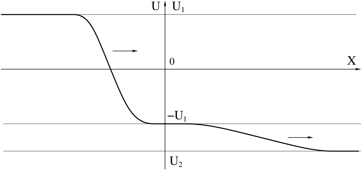
We have to say now that the step-like initial conditions of the second type (the bottom of Fig. 19) can be investigated just by the change .
Let us mention here also the very interesting solutions of (57) including the soliton part and solution (59). The soliton solutions coexist with solution (59) and the interaction of a soliton with (59) results in the phase shift and the soliton ”flip” (Fig. 22).

Finally, we point out again that while considerations above were given for the function , representing Riemann invariants , we can express the results in terms of physical variables and using equation (29) (we also remind the readers that our analysis assumes the limit and ). We find that for (Fig. 23) the case
corresponds to the case , . For we also have , (see Fig. 23). It is not difficult to see that conditions of this type can arise naturally after separating the right- and left-moving parts of initial conditions, as shown in Fig. 24 .


References
- [1] M.J. Ablowitz, H. Segur. Solitons and the Inverse Scattering Transform. Society for Industrial and Applied Mathematics (SIAM), Philadelphia, 1981.
- [2] Ahufinger, V. and Sanpera, A. and Pedri, P. and Santos, L. and Lewenstein, M., Creation and mobility of discrete solitons in Bose-Einstein condensates, Phys. Rev. A 69 : 5 (2004), 053604.
- [3] Ahufinger, V. and Sanpera, A., Lattice Solitons in Quasicondensates, Phys. Rev. Lett. 94 : 13 (2005), 130403.
- [4] Altman, E. and Polkovnikov, A. and Demler, E. and Halperin, B. I. and Lukin, M. D., Superfluid-Insulator Transition in a Moving System of Interacting Bosons, Phys. Rev. Lett. 95 : 2 (2005), 020402.
- [5] W. Bakr et al., Nature 462 (2009), 74.
- [6] Benjamin, T.B. and Feir, J.E., The disintegration of wave trains on deep water. Part 1. Theory. J. Fluid Mech. 27 (1967) 417-430. Feir, J.E. Discussion: Some results from wave pulse experiments, Proc. R. Soc. Lond. A 299 (1967) 54-58.
- [7] V. I. Bespalov and V. I. Talanov. JETP Letters. 3 (1966), 307.
- [8] E. Bettelheim, A. G. Abanov, P. Wiegmann. Orthogonality catastrophe and shock waves in a non-equilibrium Fermi gas. arXiv:cond-mat/0607453 , Phys. Rev. Lett. 97, 246402 (2006).
- [9] E. Bettelheim, A. G. Abanov, P. Wiegmann. Quantum Shock Waves - the case for non-linear effects in dynamics of electronic liquids. arXiv:cond-mat/0606778 , Phys.Rev.Lett. 97 (2006) 246401.
- [10] E. Bettelheim, A. G. Abanov, P. Wiegmann. Nonlinear Dynamics of Quantum Systems and Soliton Theory. arXiv:nlin/0605006 , J.Phys. A40 (2007) F193-F208 .
- [11] Borgad L.A., Its A.R., Matveev V.B., Manakov S.V., Zakharov V.E. Phys. Lett. bf 63 A, N 3 (1979) p. 205.
- [12] I. Bloch, Nature Physics 1 (2005), 23.
- [13] Bloch, Immanuel and Dalibard, Jean and Zwerger, Wilhelm, Many-body physics with ultracold gases, Rev. Mod. Phys. 80 : 3 (2008), 885–964.
- [14] I. Bloch, Science 319 (2008), 1202.
- [15] Burger, S. and Bongs, K. and Dettmer, S. and Ertmer, W. and Sengstock, K. and Sanpera, A. and Shlyapnikov, G. V. and Lewenstein, M., Dark Solitons in Bose-Einstein Condensates, Phys. Rev. Lett. 83 : 25 (1999), 5198–5201.
- [16] Y. Castin, Eur. Phys. Journal B 68 (2007), 556.
- [17] A. Daley et al., Journal of Statistical Mechanics: Theory and Experiment, 2004 : 4 (2004), 04005.
- [18] Damski, B. and Zakrzewski, J. and Santos, L. and Zoller, P. and Lewenstein, M., Atomic Bose and Anderson Glasses in Optical Lattices, Phys. Rev. Lett. 91 : 8 (2003), 080403.
- [19] J. Denschlag et al., Science 287 (2000), 97.
- [20] V.S. Druma, On analytic solution of the two-dimensional Korteweg-de Vries equation, JETP Lett., 19 : 12 (1974), 219-225.
- [21] Duan, L.-M. and Demler, E. and Lukin, M. D., Controlling Spin Exchange Interactions of Ultracold Atoms in Optical Lattices, Phys. Rev. Lett. 91 : 9 (2003), 090402.
- [22] Eiermann, B. and Anker, Th. and Albiez, M. and Taglieber, M. and Treutlein, P. and Marzlin, K.-P. and Oberthaler, M. K., Bright Bose-Einstein Gap Solitons of Atoms with Repulsive Interaction, Phys. Rev. Lett. 92 : 23 (2004), 230401.
- [23] Fallani, L. and De Sarlo, L. and Lye, J. E. and Modugno, M. and Saers, R. and Fort, C. and Inguscio, M., Observation of Dynamical Instability for a Bose-Einstein Condensate in a Moving 1D Optical Lattice, Phys. Rev. Lett. 93 : 14 (2004), 140406.
- [24] E. Fermi, J.R. Pasta, and S. Ulam. ”Studies of Nonlinear Problems I.”, Los Alamos Report No. LA-1940, 1955.
- [25] E. Fradkin, Field Theories of Condensed Matter Systems, Addison-Wesley Publishing Company (1991).
- [26] I.M. Gelfand, B.M. Levitan., Izvestia Akad. Nauk S.S.S.R., Ser. Math. 15 (1951), 309.
- [27] N. Gemelke et al., Nature 460 (2009), 995.
- [28] G.S. Gardner, J.M. Green, M.D. Kruskal, R.M. Miura. Phys. Rev. Lett. 19 , 1095 (1967).
- [29] T. Giamarchi, Quantum Physics in One dimension, Oxford Science Publishing (2004).
- [30] M. Greiner and S. Foelling, Nature 453 (2008), 736.
- [31] M. Greiter and F. Wilczek and E. Witten, Mod. Phys. Lett. 3 (1989), 405.
- [32] A.V. Gurevich, L.P. Pitaevskii., Decay of initial discontinuity in the Korteweg - de Vries equation, JETP Letters 17 (1973), 193-195.
- [33] A.V. Gurevich, L.P. Pitaevskii., Nonstationary structure of a collisionless shock waves, Sov. Phys. JETP 38 (1974), 291-297.
- [34] Haller et al., Science 325 (2009), 1224.
- [35] Halperin, B. I. and Hohenberg, P. C., Hydrodynamic Theory of Spin Waves, Phys. Rev. 188 (1969), 898–918.
- [36] Heine et al., New J. Phys. 12 (2010), 65036.
- [37] Hofferberth et al., Nature Physics 449 (2007), 324.
- [38] Hofferberth et al., Nature Physics 4 (2008), 489.
- [39] Huber, S. D. and Altman, E. and Büchler, H. P. and Blatter, G., Dynamical properties of ultracold bosons in an optical lattice, Phys. Rev. B 75 : 8 (2007), 085106.
- [40] Huber, S. D. and Theiler, B. and Altman, E. and Blatter, G., Amplitude Mode in the Quantum Phase Model, Phys. Rev. Lett. 100 : 5 (2008), 050404.
- [41] R. Jackiw and A. Kerman, Time-dependent variational principle and the effective action, Physics Letters A 71 : 2-3 (1979), 158 - 162.
- [42] D. Jaksch and P. Zoller, Annals of Physics 315 (2005), 52.
- [43] Johansson, Magnus and Kivshar, Yuri S., Discreteness-Induced Oscillatory Instabilities of Dark Solitons, Phys. Rev. Lett. 82 : 1 (1999), 85–88.
- [44] Kadomtsev, B. B., Petviashvili, V. I. ”On the stability of solitary waves in weakly dispersive media”. Sov. Phys. Dokl. 15 (1970), 539-541.
- [45] Karski, M. and Förster, L. and Choi, J. M. and Alt, W. and Widera, A. and Meschede, D., Nearest-Neighbor Detection of Atoms in a 1D Optical Lattice by Fluorescence Imaging, Phys. Rev. Lett. 102 : 5 (2009), 053001.
- [46] I. Kay, H.E. Moses, Nuovo Cimento 3 (1956), 276; J. Appl. Phys. 27 (1956), 1503.
- [47] Kevrekidis, P. G. and Carretero-González, R. and Theocharis, G. and Frantzeskakis, D. J. and Malomed, B. A., Stability of dark solitons in a Bose-Einstein condensate trapped in an optical lattice, Phys. Rev. A 68 : 3 (2003), 035602.
- [48] I. Khalatnikov and V.V. Lebedev, J. Low Temp. Phys. 32 (1978), 789.
- [49] L. Khaykovich et al., Science 287 (2002), 97.
- [50] T. Kinoshita et al., Nature 440 (2006), 900.
- [51] Kivshar, Yuri S. and Malomed, Boris A., Dynamics of solitons in nearly integrable systems, Rev. Mod. Phys. 61 : 4 (1989), 763–915.
- [52] Kuklov, A. B. and Svistunov, B. V., Counterflow Superfluidity of Two-Species Ultracold Atoms in a Commensurate Optical Lattice, Phys. Rev. Lett. 90 : 10 (2003), 100401.
- [53] Palzer, Stefan and Zipkes, Christoph and Sias, Carlo and Köhl, Michael, Quantum Transport through a Tonks-Girardeau Gas, Phys. Rev. Lett. bf 103 : 15 (2009), 150601.
- [54] M.D. Kruskal, N.J. Zabusky. Stroboscopic-Perturbation Procedure for Treating a Class of Nonlinear Wave Equations. Journ. of Math. Phys. 5 : 2 (1964), 231 - 244.
- [55] K. Krutitsky et al., arXiv:0907.0625 (2010).
- [56] T. Lahaye et al., Reports on Progress in Physics 72 (2007), 126401.
- [57] Lancaster, Jarrett and Mitra, Aditi, Quantum quenches in an spin chain from a spatially inhomogeneous initial state, Phys. Rev. E 81 : 6 (2010), 061134.
- [58] P.D. Lax. Comm. Pure Appl. Math. 21, 467 (1968).
- [59] P.D. Lax, C.D. Levermore., The small dispersion limit for the Korteweg - de Vries equation I, II, and III. Comm. Pure Appl. Math., 36 (1983), 253-290, 571-593, 809-830.
- [60] P.D. Lax, C.D. Levermore, S. Venakides., The generation and propagation of oscillations in dispersive IVPs and their limiting behavior, Important developments in soliton theory 1980-1990, 205-241, Springer Series in Nonlinear Dynamics. Springer, Berlin (1993).
- [61] M. Lewenstein et al., Advances in Physics 56 (2007), 243.
- [62] M.J. Lighthill, Proc. Roy. Soc. A299 (1967), 28.
- [63] V.A. Marchenko, Doklady. Akad. Nauk SSSR 104 (1955), 695.
- [64] T. Maxworthy, L.G. Redekopp., Icarus 29, 261 (1976).
- [65] Miles J.W. Resonantly interacting solitary waves. J. Fluid Mech. 79 (1977), 171-179.
- [66] R.M. Miura. Korteweg - de Vries equation and generalizations. I. A remarkable explicit nonlinear transformation. - J. Math. Phys. 9, 1202 -1204 (1968).
- [67] Mun, Jongchul and Medley, Patrick and Campbell, Gretchen K. and Marcassa, Luis G. and Pritchard, David E. and Ketterle, Wolfgang, Phase Diagram for a Bose-Einstein Condensate Moving in an Optical Lattice, Phys. Rev. Lett. 99 : 15 (2007), 150604.
- [68] Murg, V. and Verstraete, F. and Cirac, J. I., Variational study of hard-core bosons in a two-dimensional optical lattice using projected entangled pair states, Phys. Rev. A 75 : 3 (2007), 033605.
- [69] Naumkin and Shishmarev, The step-decay problem for the Korteweg-de Vries-Burgers equation, Functional Analysis and Its Applications 25 : 1 (1991), 16-25.
- [70] K. Nelson and X. Li and D. Weiss, Nature Phys. 3 (2007), 556.
- [71] A. C. Newell, Solitons in mathematics and physics. Society for Industrial and Applied Mathematics (1985).
- [72] S.P. Novikov, S.V. Manakov, L.P. Pitaevskii, and V.E. Zakharov., Theory of solitons. The inverse scattering method., Plemun, New York 1984.
- [73] L. Ostrovsky and A. Potapov, Modulated Waves. Theory and applications., The Johns Hopkins University Press (1999).
- [74] H. Ott et al., Nature Phys. 4 (2008), 949.
- [75] T.L. Perelman, A. Kh. Fridman, M.M. Yelyashevich. Modified Korteweq - de Vries equation in electrohydrodynamics. Sov. Phys. JETP. 39 (1974a), 643-646.
- [76] L. Pitaevskii and S. Stringari, Bose-Einstein Condensation, Oxford Science Publications (2002)
- [77] Polkovnikov, A. and Altman, E. and Demler, E. and Halperin, B. and Lukin, M. D., Decay of superfluid currents in a moving system of strongly interacting bosons, Phys. Rev. A 71 : 6 (2005), 063613.
- [78] Ritter, Stephan and Öttl, Anton and Donner, Tobias and Bourdel, Thomas and Köhl, Michael and Esslinger, Tilman, Observing the Formation of Long-Range Order during Bose-Einstein Condensation, Phys. Rev. Lett. 98 : 9 (2007), 090402.
- [79] N. N. Romanova. N-Soliton solution on a pedestal of the modified Korteweg-de Vries equation. - Theor. and Math. Phys. 39 : 2 (1979), 415-421.
- [80] Satsuma J. -soliton solution of the two-dimensional Korteweg - de Vries equation. J. Phys. Soc. Japan. 40 (1976), 286-290.
- [81] L. Sadler et al., Nature 443 (2006), 312.
- [82] Scalettar, R. T. and Batrouni, G. G. and Kampf, A. P. and Zimanyi, G. T., Simultaneous diagonal and off-diagonal order in the Bose-Hubbard Hamiltonian, Phys. Rev. B 51 : 13 (1995), 8467–8480.
- [83] Scarola, V. W. and Das Sarma, S., Quantum Phases of the Extended Bose-Hubbard Hamiltonian: Possibility of a Supersolid State of Cold Atoms in Optical Lattices, Phys. Rev. Lett. 95 : 3 (2005), 033003.
- [84] U. Schneider et al., Breakdown of diffusion: From collisional hydrodynamics to a continuous quantum walk in a homogeneous Hubbard model, arXiv:1005.3545, 2010.
- [85] Schmid, Guido and Todo, Synge and Troyer, Matthias and Dorneich, Ansgar, Finite-Temperature Phase Diagram of Hard-Core Bosons in Two Dimensions, Phys. Rev. Lett. 88 : 16 (2002), 167208.
- [86] Schollwöck, U., The density-matrix renormalization group, Rev. Mod. Phys. 77 : 1 (2005), 259–315.
- [87] Sherson et al., Nature 467 (2010), 68.
- [88] Strohmaier, Niels and Greif, Daniel and Jördens, Robert and Tarruell, Leticia and Moritz, Henning and Esslinger, Tilman and Sensarma, Rajdeep and Pekker, David and Altman, Ehud and Demler, Eugene., Phys. Rev. Lett. 104 : 8 (2010), 080401.
- [89] B. Sutherland, Beautiful Models, World Scientific (2004).
- [90] Trombettoni, Andrea and Smerzi, Augusto, Discrete Solitons and Breathers with Dilute Bose-Einstein Condensates, Phys. Rev. Lett. 86 : 11 (2001), 2353–2356.
- [91] S. Trotzky et al., Science 319 (2008), 295.
- [92] M. Wadati. J. Phys. Soc. Japan 34, 1289 (1973).
- [93] X.G. Wen, Advances in Physics 44 (1995), 405.
- [94] Wu, Biao and Niu, Qian, Landau and dynamical instabilities of the superflow of Bose-Einstein condensates in optical lattices, Phys. Rev. A 64 : 6 (2001), 061603.
- [95] Yulin, Alexey V. and Skryabin, Dmitry V., Out-of-gap Bose-Einstein solitons in optical lattices, Phys. Rev. A 67 : 2 (2003), 023611.
- [96] N.J. Zabusky. Phenomena Associated with the oscillations of a Nonlinear Model String. In Proceedings of the Conference on Mathematical Models in the Physical Sciences, edite by Stefan Drobot (Prentice - Hall, Inc. New York, 1963), p. 99.
- [97] N.J. Zabusky and M.D. Kruskal. Interaction of ”solitons” in a collisionless plasma and the recurrence of initial states. Phys. Rev. Lett. 15 : 6 (1965), 240-243.
- [98] V.E. Zakharov, S.V. Manakov., Asymptotic behavior of nonlinear wave systems integrated by the inverse scattering method., Sov. Phys. JETP 44 (1) (1976), 106-112.
- [99] V. E. Zakharov and A. B. Shabat, Interaction between solitons in a stable medium. Sov. Phys. JETP 37, 823-828 (1973).
- [100] V. E. Zakharov and A. B. Shabat, Integration method of nonlinear equations of mathematical physics with the help of the inverse scattering problem, Funk. Anal Pril., 8 : 3 (1974), 43-53.
- [101] Zakrzewski, Jakub, Mean-field dynamics of the superfluid-insulator phase transition in a gas of ultracold atoms, Phys. Rev. A 71 : 4 (2005), 043601.
- [102] Zimmermann et al., arXiv:1011.1004 (2010).