Thermodynamics of Trapped Imbalanced Fermi Gases at Unitarity
Abstract
We present a theory for the low-temperature properties of a resonantly interacting Fermi mixture in a trap, that goes beyond the local-density approximation. The theory corresponds essentially to a Landau-Ginzburg-like approach that includes self-energy effects to account for the strong interactions at unitarity. We show diagrammatically how these self-energy effects arise from fluctuations in the superfluid order parameter. Gradient terms of the order parameter are included to account for inhomogeneities. This approach incorporates the state-of-the-art knowledge of the homogeneous mixture with a population imbalance exactly and gives good agreement with the experimental density profiles of Shin et al. [Nature 451, 689 (2008)]. This allows us to calculate the universal surface tension of the interface between the equal-density superfluid and the partially polarized normal state of the mixture. We also discuss the possibility of a metastable state to explain the deformation of the superfluid core that is seen in the experiment of Partridge et al. [Science 311, 503 (2006)].
1 Introduction
Ultracold atom experiments are always performed in a trap to avoid contact of the atoms with the ‘hot’ material walls that would heat up the cloud. Due to this trapping potential the atomic cloud is never homogeneous. However, typically the energy splitting of the trap corresponds to a small energy scale, so that the inhomogeneity is not very severe. In this case, we may use the so-called local-density approximation (LDA). It physically implies that the gas is considered to be locally homogeneous everywhere in the trap. The density profile of the gas is then fully determined by the condition of chemical equilibrium, which causes the edge of the cloud to follow an equipotential surface of the trap.
But even if the trap frequency is small, the LDA may still break down. An important example occurs when an interface is present in the trap due to a first-order phase transition. For a resonantly interacting Fermi mixture with a population imbalance in its two spin states [1, 2], such interfaces were encountered in the experiments by Partridge et al. [2] and by Shin et al. [3] at sufficiently low temperatures. Here the LDA predicts the occurrence of a discontinuity in the density profiles of the two spin states, which cost an infinite amount of energy when gradient terms are taken into account. Experimental profiles are therefore never truly discontinuous, but are always smeared out. An important goal of this chapter is to address this interesting effect, which amounts to solving a strongly interacting many-body problem beyond the LDA. Due to the rich physics of the interface, new phases can be stabilized that are thermodynamically unstable in the bulk. This exciting aspect shares similarities with the physics of superfluid helium-3 in a confined geometry [4] and spin textures at the edge of a quantum Hall ferromagnet [5].
Note that the presence of an interface also can have further consequences. Namely, in a very elongated trap, Partridge et al. observed a strong deformation of the minority cloud at their lowest temperatures. At higher temperatures the shape of the atomic clouds still followed the equipotential surfaces of the trap [6]. A possible interpretation of these results is that only for temperatures sufficiently far below the tricritical point [3, 7, 8, 9, 10, 11], the gas shows a phase separation between a balanced superfluid in the center of the trap and a fully polarized normal shell around this core. The superfluid core is consequently deformed from the trap shape due to the surface tension of the interface between the two phases [6, 12, 13]. This causes an even more dramatic breakdown of the LDA. Although the above interpretation leads to a good agreement with the experiments of Partridge et al. [6], a microscopic understanding of the value of the surface tension required to explain the observed deformations has still not been obtained. Presumably closely related to this issue are a number of fundamental differences with the study by Shin et al. [3]. Most importantly, the latter observes no deformation and finds a substantially lower critical polarization, which agrees with Monte Carlo calculations combined with a LDA. It appears that the interfaces between the superfluid core and the normal state are fundamentally different for the two experiments, which might play an important role in resolving the remaining discrepancies. In order to investigate this interface we need to go beyond the local-density approximation.
To study the details of the superfluid-normal interface we need a theory that can describe the inhomogeneous and population imbalanced unitarity Fermi gas. For this, we first need a theory that includes in the homogeneous case both the normal state and the superfluid state in one quantitative correct description. Secondly, we need to incorporate the inhomogeneous effects of the trapping potential. The aim of this chapter is to give a simple and elegant way to achieve this. In the following two sections, we fist arrive at an accurate, and to a large extent analytical description of the thermodynamics of a population imbalanced unitarity Fermi gas. This is achieved by constructing an appropriate thermodynamic potential for the Fermi mixture at unitarity. All desired thermodynamic quantities can then be obtained by performing the appropriate differentiations of the thermodynamic potential that are well known from statistical physics. The inhomogeneity effects of the trapping potential are included by taking the energy penalty for large variations in the order parameter into account. These gradient terms smoothen the jump of the order parameter that is predicted by the LDA at the location of the first-order phase transition. We will see that this gives a more detailed explanation of the experimental data of Shin et al. [3]. In the last section we then show how the surface tension can be computed with this more detailed description of the interface. This surface tension turns out to be relatively small. This does, therefore, not explain the dramatic deformation seen in the experiment of Partridge et al. [6]. An alternative explanation may be that there exists a metastable state with a deformed superfluid core [14]. At the end of this chapter we briefly discuss this possibility. We find that the Landau-Ginzburg-like theory derived here does not appear to contain such a metastable state.
2 Ultracold Quantum Fields
In order to properly study the unitary Fermi mixture, we derive a single thermodynamic potential that in a quantitative correct manner describes both the normal and the superfluid phases. As we will see, the normal state of the unitarity Fermi mixture is straightforwardly incorporated by introducing two mean-field-like self-energies. In particular, it is possible in this manner to completely reproduce the equation of state known from Monte-Carlo calculations. However, including also the possibility of superfluidity at low temperatures and low polarizations turns out to be more difficult. To understand better how this can nevertheless be achieved, we first give an exact diagrammatic discussion of the superfluid state that is then in the next section used to arrive at the desired thermodynamic potential of the unitarity Fermi mixture.
2.1 Bardeen-Cooper-Schrieffer Theory
In this subsection we outline the basic ingredients of a field-theoretical description for the superfluid state of the imbalanced Fermi mixture [15]. We start with the essentially exact action for such an atomic two-component mixture,
| (1) | ||||
Here is the fermion field of the atomic species in the hyperfine state , is the associated chemical potential, is a Grassmann-valued current source that is convenient in the following, but which is put equal to zero at the end of the calculations, and is the strength of the unitarity-limited attractive interactions between the two species. The grand-canonical partition function is then given by
| (2) |
This represents a functional integral over all the fermion fields that are antiperiodic on the imaginary time interval , with the inverse thermal energy. The thermodynamic potential is ultimately given in terms of the partition function as
| (3) |
with the total volume of the system. To make the connection with thermodynamics explicit, we note that the thermodynamic potential is related to the pressure of the gas by means of .
In order to describe pairing of the fermions, we perform a Hubbard-Stratonovich transformation to the complex pairing field . For this field we have that
| (4) |
This transformation makes the action quadratic in the fermion fields. More precisely, we have that
| (5) | ||||
where we defined and , which are vectors in a two-dimensional space, known as Nambu space. In this space the Green’s function matrix is given by . The first term in the right-hand side represents the noninteracting part and is given by
| (6) | ||||
| with the noninteracting Green’s function of species . The second term corresponds to the BCS self-energy, which has only off-diagonal terms and reads | ||||
| (7) | ||||
The action now only contains quadratic terms in the fermion fields, which is something we can handle exactly. However, the tradeoff is an extra functional integral over the field. Starting with the easy part, we perform the functional integral over the fermion fields. Since this is a standard Gaussian integral, we immediately obtain
| (8) | ||||
where the trace implies a summation over the Nambu space indices as well as an integral over position and imaginary time. The second term in the action contains all orders in and as a result the theory is thus still very complex and impossible to solve completely. In BCS theory, we make a saddle-point approximation and replace the pairing field by its expectation value. In other words, we write , with the expectation value and representing the fluctuations, and subsequently neglect these fluctuations. The actual value of the BCS gap can then be determined by the gap equation in Eq. (4), which is equivalent to , and is to be solved selfconsistently. This procedure is of course only valid when the interaction strength is sufficiently small.
2.2 Fluctuations
But what happens when the interaction strength is not small, as is the case at unitarity? In that case we cannot neglect the fluctuations. To deal with that situation we use in Sec. 3.2 an approach inspired by Landau-Ginzburg theory, in which we try to find an accurate self-energy matrix for the fermions that effectively takes all fluctuation effects into account. In particular we need two self-energies that contribute to the diagonal part of the exact inverse Green’s function matrix , because otherwise the normal state would correspond to an ideal Fermi mixture, which at unitarity is not an accurate starting point for a discussion of the instability towards superfluidity. However, the effective interaction between the two atomic species is not the same in the normal and superfluid states of the gas. Therefore, also this diagonal part of the self-energy must sufficiently deep in the superfluid state depend on the expectation value of the pairing field or gap and it is important to understand how this dependence precisely comes about. In this section we show that in principle all interaction effects can indeed be included in a self-energy matrix, and that also the diagonal part of this self-energy depends explicitly on the gap. A nice and insightful way to achieve this is by considering the appropriate Feynman diagrams.
The diagonal parts of the Green’s function matrix, i.e., and , are dressed by the pairing field . This is described by the Dyson equation. This Dyson equation follows from inverting the relation and can be written as
| (9) |
Diagrammatically the diagonal part of this equation can be represented in the following way,
| (10) | ||||
Here the dashed line represents the pairing field and the direction of the arrow depicts the difference between and . The solid line represents the noninteracting fermionic propagators , where in this case the direction of the arrow depicts alternatingly the propagator of the two different fermion species. The first line of the equation shows the recurrence relation for the full diagonal propagator and the second line shows the first three elements originating from this Dyson equation by iteration.
In the superfluid state, the pairing field has a nonzero expectation value . In a mean-field approximation we neglect the fluctuations and replace by its expectation value . In this approximation the diagonal propagators reduces to the standard form known from BCS theory. However, when we take fluctuations into account we also get self-energy corrections on the noninteracting fermion propagators in the Dyson equation. This follows directly from the definition of the exact fermionic propagators,
| (11) | ||||
and similarly for . In BCS mean-field theory we thus have , but at unitarity we still have to perform a functional integral over the pairing field to obtain the exact results.
We can represent this functional integral over the fluctuations diagrammatically by connecting some of the fields with the pair propagator, which is determined by the effective action , put the other fields equal to the expectation value , and then sum over all possible diagrams. Because of the U(1) symmetry of the effective action, we can only draw a pair propagator between a and a , as suggested by the arrows. The fully dressed diagonal propagators now become,
| (12) | ||||
Here the connected dashed lines represent the pair propagator and the cross represents the expectation value. This series can be resummed such that we get the exact Dyson equation
| (13) |
but now with an exact self-energy matrix , which contains both diagonal (normal) and off-diagonal (anomalous) elements. For instance, the second and fifth terms drawn in the right-hand side of Eq. (12) contribute to the diagonal self-energy, whereas the last term leads to an additional contribution to the off-diagonal self-energy. These terms thus renormalize the BCS self-energy that is obtained from Eq. (7) by replacing by . From the expectation values of the gap inside the loops in Eq. (12), we explicitly see that the normal self-energies can be written as a series expansion in . The same is in fact also true for the first diagram in the right-hand side of Eq. (12), because the nonlinearities in the effective action make sure that the pair propagator already contains all orders of . These nonlinearities also lead to more complicated Feynman diagrams containing higher-order (connected) correlation functions of the pair field that are not shown here, but this does not affect our main conclusions.
We just showed that fluctuation effects of the pair field can be incorporated in an effective self-energy. The same discussion can be carried out for the gap equation. This can also be very nicely illustrated diagrammatically. The gap equation in Eq. (4) is an equation between the expectation value of the gap and the off-diagonal or anomalous propagator. We can again use the Dyson equation in Eq. (9) for the anomalous propagator to study the effects of the fluctuations on the gap equation,
|
(14) |
![[Uncaptioned image]](1102.3320v1/GapEq_open_00.png)
![[Uncaptioned image]](1102.3320v1/GapEq_open_01.png)
![[Uncaptioned image]](1102.3320v1/GapEq_open_02.png)
![[Uncaptioned image]](1102.3320v1/GapEq_open_03.png)
Here the small dot on the left of all diagrams represents the fact that the gap only depends on one space-time point, i.e., due to the point-like and instantaneous nature of the attractive interaction.
The fluctuation effects follow again from performing the functional integral over the field, since from Eq. (4) we have that
| (15) | ||||
The diagrammatic representation of this equation follows from connecting some of the pair lines in Eq. (14). Again also higher-order correlation functions of the pair field contribute, but for simplicity we do not consider these as they do not change our results. When we carry out this procedure we obtain
|
(16) |
![[Uncaptioned image]](1102.3320v1/GapEq_fluc_00.png)
![[Uncaptioned image]](1102.3320v1/GapEq_fluc_g_01.png)
![[Uncaptioned image]](1102.3320v1/GapEq_fluc_glp_02.png)
![[Uncaptioned image]](1102.3320v1/GapEq_fluc_lpglp_03.png)
![[Uncaptioned image]](1102.3320v1/GapEq_fluc_llgpp_03.png)
Notice that all terms are now proportional to instead of . The first three terms in the right-hand side can again be incorporated in a fully dressed fermion propagator by resumming this series. The last term, which for the gap equation behaves as a vertex correction, is then again incorporated into the anomalous self-energy.
In the unitarity limit, these vertex corrections are important to find the correct gap equation and, therefore, the expectation value for the gap. Also the diagonal part of the self-energy is important for a determination of the energy and the densities of the Fermi mixture. There is, however, no clear-cut way do derive these full self-energies from first principles for the unitarity case. In this chapter, we therefore use a more top-down approach. We will use the fact that these self-energies exist and can be expanded in powers of . Moreover, our previous renormalization group theory [11] has shown that for thermodynamic quantities the self-energies can in a good approximation be considered to be momentum and frequency independent. Combining these observations we are ultimately able to derive an accurate approximation to the thermodynamic potential of the unitarity Fermi mixture.
3 The Thermodynamic Potential
In the previous section we showed that interaction effects in the unitary Fermi gas can be described by including appropriate normal and anomalous self-energies into the theory. We also discussed that this, in principle well-known fact, can be understood as an effect of pair fluctuations. As a result the self-energies, and in particular the normal self-energies, depend on the gap . In addition, we showed also that the gap equation contains vertex corrections, which cannot be incorporated by dressing the diagonal propagators alone. This is one important reason for deriving also the gap equation from the thermodynamic potential, because the minimization condition then automatically generates the correct vertex corrections. For our purposes it is therefore crucial to realize that in principle there exists an exact thermodynamic potential that describes the full thermodynamics of the unitarity-limited Fermi gas. It is, however, impossible to derive this from first principles for this strongly interacting system, and we therefore have to find an appropriate approximation. In this section we will show how to arrive at such an accurate approximation to the exact thermodynamic potential.
3.1 Normal State
Despite the strong interaction, it is now rather well established that BCS mean-field theory gives the correct qualitative description of the unitarity limit, at least at the temperatures accessible to the state-of-the-art experiments. Therefore a reasonable starting point for the approximation of the thermodynamic potential is this mean-field theory. From experiments, renormalization group theory, and several Monte-Carlo calculations it is found that the phase diagram has the following features, as illustrated in Fig. 1. At zero temperature both experiments and theoretical calculations find a first-order phase transition at a local critical polarization . In the balanced situation both find a second-order transition at a critical temperature of about [16]. These second and first-order transition lines should then be connected by a tricritical point, which is confirmed in experiments and by renormalization group theory.

The thermodynamic potential in BCS theory leads to exactly the same qualitative behavior of the phase diagram, although the critical temperatures and critical polarizations are off by almost an order of magnitude and would not be visible in the window shown in Fig. 1. We therefore start with BCS theory, after which we systematically include the dominant interaction effects that are still missing. At unitarity the BCS energy functional is
| (17) | ||||
where , is the atomic mass, and the superfluid dispersion is given by the well-known BCS formula, . The second term in the right-hand side contains also a sum over the pseudospin projection , and represents the contribution due to an ideal gas of quasiparticles with the quasiparticle dispersion of the two spin states given by . Finally, we introduced the average chemical potential and half the chemical potential difference that acts as an effective magnetic field on the pseudospin as the quasiparticle dispersion clearly shows.
In BCS theory, the normal state is treated as an ideal Fermi gas, thus no interactions are taken into account. This is not correct in the unitarity limit. As discussed above, these interaction effects can be described by two self-energies. The imbalanced normal phase in the unitary limit, has been studied with Monte Carlo methods [17]. From this, the equation of state can be determined. If we can find the self-energies such that it reproduces the same equation of state for the theory, we have effectively taken all interaction effect in the normal phase into account.
For momentum and frequency independent self-energies, the self-energies can be incorporated in the theory of an ideal Fermi gas, by just changing the chemical potential. We thus replace the chemical potentials as
| (18) |
Here is the effective chemical potential and the self-energy for species . Inspired by Hartree-Fock theory we would write down an ansatz for the self-energy of species that is proportional to the density of species [10]. However, the densities are in a grand-canonical setting calculated by taking the derivative of with respect to the chemical potentials, i.e., . It is therefore preferable to write the self-energies as a function of the chemical potentials only. By considering terms with the correct units that incorporate the Hartree-Fock-like feature mentioned above, we find that the following self-energies gives rise to the correct equation of state of the strongly interacting normal phase,
| (19) |
The prefactor can be determined from the self-energy of a single minority atom in the presence of a Fermi sea of majority atoms and equals [17, 18, 19, 11]. Explicitly in terms of and , these relations imply that
| (20) | ||||
In Fig. 2 the resulting energy of the mixture determined from the thermodynamic potential at zero temperature is plotted as a function of the polarization. This figure shows the excellent agreement between the Monte-Carlo data and the ansatz from Eq. (20). In the next section we discuss how these self-energies can be further improved when we also consider the effects of pairing in the superfluid state.

3.2 Superfluid State
When the temperature is low enough and the imbalance not too large, the unitary Fermi gas becomes superfluid. In the unitarity limit, the scattering length goes to infinity and is no longer a relevant length scale. In fact, in the homogeneous situation, the (average) Fermi energy is the only energy scale in the problem. This makes the system universal and as a result, we can write most thermodynamic properties of the system in terms of this Fermi energy [18].
In Sec. 2 we showed that the self-energies can be explicitly written as a power series in . The straightforward first step to incorporate these superfluid gap corrections to the self-energy is to take the first term in into account [20]. We subtract this from the effective chemical potential in Eq. (20) as
| (21) |
and a constant to be determined next. For this we use one simple but important piece of information, namely the value of the thermodynamic potential in the balanced superfluid minimum. From experiments and Monte-Carlo calculations this minimum is known to be
| (22) |
with the volume and a universal number. Matching the energy in the minimum is important, because this ensures a correct energy balance between the (imbalanced) normal state and the superfluid state and therefore the correct location of the first-order phase transition at low temperature. From experiments and several theoretical calculations, it is now believed that at low temperatures the superfluid state is balanced. Thus, to find the transition we should compare the energy in the balanced superfluid with the normal state energy, for which we have already a description that agrees with the Monte-Carlo equation of state and thus has the correct energy. This condition fixes the unknown constant to , which follows directly from the zero-temperature minimum of in Eq. (17) with both self-energy corrections subtracted from the chemical potential.
At this point our construction, where everything is explicitly written in terms of the chemical potentials and , gives rise to a problem: The superfluid in the minimum of the thermodynamic potential turns out not to be balanced at low temperatures for . This problem originates from the normal self-energies in Eq. (20) which explicitly depends on the chemical potential difference . It is in particular the renormalization of the average chemical potential which depends on , thus . This problem could have been avoided by making an ansatz in terms of the densities instead of the chemical potentials, which would automatically have resulted in a balanced superfluid [21]. This follows directly from the fact that BCS theory already gives a balanced superfluid at low temperature and the dependence on imbalance in the self-energies is thus suppressed in the superfluid state. Physically, the problem is that the formation of a Bose-Einstein condensate of Cooper pairs gives the superfluid state a strong preference for equal densities of the two spin states, which is not present in the normal state. To incorporate this extra piece of physics into the theory, we need to add an extra dependence to the model to ensure a balanced superfluid in the minimum of the thermodynamic potential. There are several ways to achieve this, but an exponential suppression of the dependence in turns out to give the best interpolation between the various known regimes. Technically this is achieved, by replacing in by . The factor of in the exponent is somewhat arbitrary, but should be large enough to make the dependence in the ground-state superfluid minimum negligible.
We now have included the self-energy effects in both the normal state as well as in the superfluid state. This results in an approximation for the thermodynamic potential which has the correct equation of state in the normal phase, the correct energy minimum for the superfluid phase, and interpolates between these two in a manner that incorporates all the known physical properties of the system. In Fig. 3 the resulting thermodynamic potential is plotted for several values of and at zero temperature. As a check we can compute the critical polarization which gives about as desired. Also the universal number of the balanced superfluid ground state has a very reasonable value. Here we find while Monte Carlo gives [22, 23]. In principle, we can easily correct for this difference by including a small correction to the anomalous self-energy, but in view of the already rather good agreement with the Monte-Carlo results we refrain from doing so in the following.
t]

A large region of the trapped unitary Fermi gas can be well described using the local-density approximation. However, near the interface of a first-order phase transition, this approximation always breaks down, as it leads to an unphysical discontinuity in the density profiles. The thermodynamic potential we constructed so far also describes the system out of equilibrium, i.e., with not in a minimum of the thermodynamic potential, which is precisely what happens near the interface. But in order to describe the interface properly, we need to go beyond the LDA by including also a gradient term for in the thermodynamic potential,
| (23) |
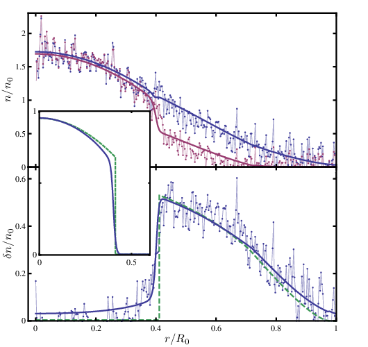
where denoted the homogeneous thermodynamic potential density and is a positive function of the ratio only, due to the universal nature of the Fermi mixture at unitarity. The functional minimum of this new thermodynamic potential gives a smooth transition at the interface, instead of the discontinuous step obtained within the LDA. A careful inspection of the interface in the data of Shin et al. [3], cf. Fig. 4, also reveals that the interface is not a sharp step. This is most clear in the data for the density difference, since the noise in the density difference is much smaller than in the total density. This has to do with the experimental procedure used, which only measures the density difference directly. Such a smooth transition arises also in the self-consistent Bogoliubov-de Gennes equations. But these lead then also to oscillations in the order parameter and the densities, due to the proximity effect [24]. This is not observed experimentally. Oscillations will also occur in our Landau-Ginzburg approach if . However, we have checked both with the above theory as well as with renormalization group calculations [11] that is positive. This agrees with the phase diagram of the imbalanced Fermi mixture containing a tricritical point and not a Lifshitz point in the unitarity limit [25].
We restrict ourselves here to a gradient term that is of second order in and also of second order in the gradients. There are of course higher-order gradient terms that may contribute quantitatively [26], but the leading-order physics is captured in this way due to the absence of a Lifshitz transition. One way to compute the coefficient is to use the fact that in equilibrium this coefficient can be exactly related to the superfluid stiffness, and therefore the superfluid mass density , by . At zero temperature it gives the simple result that , with and universal constants as defined earlier. With this result for our thermodynamic potential functional in Eq. (23) contains no longer any free parameters and can now be confronted with experiments. The result of this comparison, at a realistic temperature of about one third the tricritical temperature , is shown in Fig. 4 and turns out to be excellent.
4 Applications
We have thus constructed an accurate approximation to the exact thermodynamic potential of the imbalanced Fermi mixture at unitarity. With a simple ansatz for the self-energies we can describe both the homogeneous normal and superfluid phase at zero and nonzero temperatures. Moreover, the description is also valid out of equilibrium, i.e., when the value of the gap is not in a minimum of the thermodynamic potential. By including also the energy cost for gradients of the gap parameter we have a Landau-Ginzburg-like theory that can describe the inhomogeneous situation that is used in experiments [2, 3] in a manner that goes beyond the local-density approximation.
In this section we use the thermodynamic potential from Eq. (23) to investigate the properties of the superfluid-normal interface. First, we consider the trap to be spherically symmetric and in that case calculate the surface tension of the interface. This is an important quantity that has been put forward [12, 2] as a possible explanation for the deformations of the superfluid core observed by Partridge et al. [2]. Second, we then show how the anisotropy of the trap can be incorporated and study the effect of this anisotropy on the equilibrium gap profile . In this section we for simplicity always take the gap to be real, which does not lead to any loss of generality for the applications that we consider here.
4.1 Interface and Surface Tension
The fact that we are able to study the superfluid-normal interface beyond the LDA, makes it possible for us to also determine the surface tension. The surface tension is determined by the difference in thermodynamic potential between a one-dimensional LDA result with a discontinuous step in and our Landau-Ginzburg theory with a smooth profile for the order parameter . In actual experiments, however, the width of the interface is rather small compared to the size of the whole atomic cloud. This makes it possible to compute the surface tension by considering a flat interface in a homogeneous system rather than a curved interface in the trap. In the homogeneous case, such an interface occurs only when the imbalance is critical, i.e., when with another universal number, for which we have obtained . This means that the thermodynamic potential of the normal state minimum is exactly equal to the thermodynamic potential of the superfluid state minimum. The surface tension is then the difference in thermodynamic potential between a system that stays in one minimum and one that goes near the interface from one minimum to the other.
How the system achieves the latter is determined by minimizing the thermodynamic potential,
| (24) |
In principle, this highly nonlinear equation can be numerically solved, to get a hyperbolic tangent-like function for that on the normal side of the interface approaches zero and on the superfluid side approaches the equilibrium position of the superfluid minimum that we simply denote by . Fortunately, however, this solution is not needed to compute the surface tension, because the surface tension can be conveniently written as
| (25) |
where is the thermodynamic potential density. This equation can be rewritten as an integral over , knowing that is a monotonically increasing function between zero and . Using also the first integral of Eq. (24), we end up with
| (26) |
This is clearly independent of the actual shape of the interface. The surface tension thus only depends directly on and on the shape of the barrier in between the two minima of the thermodynamic potential. It is useful to write the surface tension in a dimensionless form. We define this as , with a dimensionless number. This number depends only on the temperature. In a trap, the relevant chemical potential is the one at the position of the interface. This location is also dependent on the polarization of the mixture and in that manner also the surface tension will inherit in a trap a dependence on the polarization [13].
The surface tension of this model is plotted in Fig. 5 as a function of the temperature. Here the surface tension is plotted in its dimensionless form. In this form it was previously found that for the experiment of Partridge et al. [6]. This was extracted from the large deformations of the superfluid core observed in that experiment. The experiment of Shin et al. does not show any deformation, which puts an upper bound on of about [13, 27]. At the tricritical point the surface tension vanishes and at zero temperature it is about . For a more realistic temperature of about we find which is significantly smaller than the surface tension that would cause a substantial deformation. This is thus in agreement with the experiment of Shin et al. [3].
We now give a more detailed discussion of our analysis of the density profiles observed by Shin et al. In experiments the cloud is trapped in an anisotropic harmonic potential, which is cigar shaped, and in the axial direction less steep than in the radial direction. However, since the atomic cloud shows no deformations in this case we can in a good approximation take the trap to be spherically symmetric. The order parameter then depends only on the radius, and the total thermodynamic potential is given by integrating our Landau-Ginzburg-like thermodynamic potential density over the trap volume. To account for the trap potential in the energy functional we let the average chemical potential depend on the radius, such that we have , with the effectively isotropic harmonic potential.

To find the order parameter as a function of the radius we have to minimize the energy functional with respect to the order parameter, or . This gives a second-order differential equation for as we have seen. Solving this Euler-Lagrange equation, with the proper boundary conditions in the center of the trap, gives a profile for that is shown in the inset of Fig. 4. This profile of the order parameter is much smoother than the discontinuous step one obtains within the LDA that is also shown in Fig. 4. Besides this, there are two more aspects that deserve some attention. First, we notice that the value of the gap at the original LDA-interface is decreased by almost a factor of three and, second, the gap penetrates into the area originally seen as the normal phase. This behavior makes the gap for a small region smaller than , giving locally rise to a gapless superfluid, which implies a stabilization of the Sarma phase.
Before discussing this particular physics, we focus first on the density difference. To obtain the density profiles within our theory, the thermodynamic relation is used, where is the density of particles in state and the associated local chemical potential. It is important that, because of the self-energy effects, we cannot use the standard BCS formulas for the density, but really have to differentiate the thermodynamic potential. In BCS theory this would of course be equivalent. Given the density profiles, the comparison between theory and experiment can be made and is ultimately shown in Fig. 4. Overall the agreement is very good. Theoretically the interface appears to be somewhat sharper than observed. This can be due to higher-order gradient terms, that are neglected in the calculation and that would give an additional energy penalty for a spatial variation of the order parameter. There are also experimental effects that could make the interface appear broader, for instance, the spatial resolution of the tomographic reconstruction or the accuracy of the elliptical averaging [28].
The Landau-Ginzburg-like approach presented here, shows some new features compared to the LDA. One interesting feature is the kink, that is visible in the majority density profile shown in Fig. 4. Notice that this kink appears before the original (LDA) phase transition from the superfluid to the normal phase. This kink signals a crossover to a new exotic phase, namely the gapless Sarma phase. Note that at zero temperature this crossover becomes a true quantum phase transition. At the crossover, the order parameter becomes smaller than the renormalized chemical potential difference and the unitarity limited attraction is no longer able to fully overcome the frustration induced by the imbalance. As a result the gas becomes a polarized superfluid. Because the gap is smaller than this corresponds to a gapless superconductor. In a homogeneous situation this can, far below the tricritical temperature, never be a stable state as shown in Fig. 1. However, because of the inhomogeneity induced by the confinement of the gas, the gap is at the interface forced to move away from the local minimum of the thermodynamic potential and ultimately becomes smaller than . The Sarma state is now locally stabilized even at these low temperatures. Notice that this is a feature of the smooth behavior of the gap and that the presence of the Sarma phase thus does not depend on the quantitative details of the energy functional .
4.2 Deformation
When the surface tension is sufficiently small or when the aspect ratio of the external potential of the system is close to one, the gap profile will closely follow the equipotential surfaces of the external trap and can be reasonably well approximated by a function of a single variable only. This can be achieved by scaling away the anisotropy of the external potential and introducing the effective radius
| (27) |
with the aspect ratio of the trap. However, when the aspect ratio is large, this might not always be valid. In the experiment of Partridge et al. [6], an aspect ratio of about 45 is used, and dramatic deviations between the equipotential surfaces and the shape of the superfluid core are observed. This can be explained by a large surface tension [13], but as we have just seen the required large value of cannot yet be understood from a microscopic theory. Another possibility is that the gas has ended up in a metastable state in which the shape of the gap parameter differs from the equipotential surfaces of the external potential [14].
The latter possibility is something that can also be investigated using the thermodynamic potential that we have just derived. To do so, we first study the linear response of the system when we also allow the gap profile to depend on more (angular) variables then the effective radius . After that we also look at gap profiles with a different aspect ratio than the external potential. It appears from our analysis that our present Landau-Ginzburg-like approach gives indeed rise to small deviations in the gap shape. However, it does not exhibit a metastable state with a deviation that is as large as seen in the experiment of Partridge et al.
Linear Response
The harmonic potential used in the experiments has an elliptical symmetry, which means that it can be written as a function of a single coordinate as defined in Eq. (27). As a consequence, the local thermodynamic potential also only depends explicitly on this . Therefore, in the local-density approximation, the gap parameter can only depend on as well. When we go beyond the LDA, by including gradient terms in the theory, this symmetry is explicitly broken.
In this section we first perform the above-mentioned scaling of the axial coordinate. After that we can treat the beyond-LDA corrections of the gap profile as perturbations on the symmetric solution that can be expanded in the form of spherical harmonics as
| (28) |
Since the trap is rotationally symmetric around the z-axis, the gap profile does not depend on the azimuthal angle and we are allowed to take in the expansion in Eq. (28). Also the mirror symmetry in the - plane causes all coefficients with odd to be zero. We will now assume that the elliptically symmetric part is much larger than the part with coefficients and for simplicity only look at the first anisotropic perturbation .
To describe the deformations we have thus chosen spherical coordinates, but with the -coordinate defined as . This coordinate system is not orthogonal and gives rise to a coupling between the spherical harmonics due to the gradient terms. The Jacobian is given by . The gradient terms in the thermodynamic potential can be written in these coordinates as
| (29) | ||||
Here we suppressed for convenience the dependence on the chemical potentials and approximated the stiffness by its value at the location of the interface, that we from now on denote simply by . The latter is a very good approximation in practice, because for the traps of interest the width of the superfluid-normal interface is much smaller that the typical length scale on which the trapping potential varies. Furthermore, we defined the various different effective stiffnesses as
| (30) |
This can naturally be extended to general , where every is coupled to , but we do not need that extension here.
As indicated above, we want to treat as a small perturbation in linear-response theory. To achieve this we need to expand the local part of the thermodynamic potential in terms of . This is straightforward and is given by,
| (31) |
We find the elliptical symmetric part of the gap by neglecting the contribution and minimizing the thermodynamic potential with respect to . This gives a spherical symmetric equation similar to Eq. (24), but now with a slightly smaller gradient coefficient, given by in Eq. (30). When we have obtained a solution for we can minimize the thermodynamic potential with respect to , which gives the following linear-response equation
| (32) |
with the linear operator
| (33) |
and the inhomogeneous term that acts as a source for the quadrupole deformations
| (34) |
In Dirac notation the solution of this equation is formally given by . Inverting the operator can be accomplished by first diagonalizing this operator, which we can do by finding all its eigenfunctions and eigenvalues. Interestingly, these are determined by a Schrödinger equation
| (35) |
with an effective mass given by and an effective potential
| (36) |
A typical example of this effective potential with its eigenstates and energies is shown in Fig. 6. Given these eigenfunctions the solution for can in Dirac notation finally be written as , which amounts to
| (37) |
In Fig. 6 also the corresponding solution for is shown. This solution is centered around the interface and is also roughly of the same width as the interface. This is as expected, since the terms in the thermodynamic potential that do not obey the elliptical symmetry and are the source for the quadrupole deformations, are most significant near the interface. Formally, this comes about because the sum in the right-hand side of Eq. (37) is, due to the energy denominator, dominated by the eigenstates with low energies that are localized in the dimple of the effective potential .


The outcome of our linear-response analysis gives only rise to small deformations from the elliptical symmetry. In fact, this a posteriori makes this approach self-consistent and confirms the assumption that the gap can be well described with a solution that has the same symmetry as the trap. While this symmetric solution gives roughly speaking the average shape of the interface, the small quadrupole deformations correct for this and widen the interface in the radial direction and shrink it in axial direction. This effect becomes bigger for larger aspect ratios, but never gives rise to such large deformations as is seen in the experiments of Partridge et al. For an aspect ratio of one, the deformation disappears, because the source term is proportional to , which becomes zero at . In principle, a deformation could then occur spontaneously, if one or more eigenvalues become negative. However, for typical experimental parameters, this never happens.
In this subsection we discussed the linear response of the superfluid-normal interface shape. This is a nice application for our Landau-Ginzburg-like thermodynamic potential functional that can be used to study in detail the effect of the aspect ratio of the trap on the experiment of Shin et al. However, we cannot use it to describe the large deformations observed by Partridge et al. A possible way to handle this situation requires beyond linear-response methods that are covered in the next section.
Metastable States
In the previous section we assumed that the deviations from the elliptically symmetric solution for the gap are small and therefore validates the use of linear response. But since we have the full thermodynamic potential at our disposal we can also consider large deviations by using a variational approach. In the experiment of Partridge et al. the observed deformation of the superfluid core is indeed large. This deformation can be modelled by giving the superfluid core a different aspect ratio than that of the trap [13] and by letting the polarized normal shell follow the shape of the trap. It is still unclear whether this represents the true energy minimum of the system or corresponds to a metastable state [14]. We can use our thermodynamic potential to investigate this, and we will see that there appears to be no metastable state in the Landau-Ginzburg-like theory presented in this chapter.
The superfluid core is described by a nonzero gap function, which is determined by minimizing the thermodynamic potential. The case of a metastable state then corresponds to a local, but not a global minimum of the thermodynamic potential. We want to find such minima by using a variational approach. This implies that we somehow have to parameterize a likely functional form of the gap, and then vary the thermodynamic potential with respect to these parameters. To find a appropriate trial function that describes the gap well, let us start with the following function that very accurately describes the gap in the elliptically symmetric case
| (38) |
Here , and are variational parameters. These parameters can be understood as follows. In the homogeneous theory the gap is proportional to the chemical potential , as discussed before, and in the trap the chemical potential is given by . This explains the first factor in the right-hand side of Eq. (38), where the parameter is needed to incorporate beyond-LDA effects. The function with center and width describes the interface profile, since this is approximately equal to the usual soliton solution for an interface in Landau-Ginzburg theory. For specific temperatures and polarizations a minimum of the thermodynamic potential with respect to these variational parameters can easily be found numerically.
Let us now also include the aspect ratio in this variational approach. We want to see how the thermodynamic potential changes when the superfluid core has a smaller aspect ratio than the normal shell. Since we consider this in a variational manner, we need a proper function with a parameter to describe this. Let us first simply vary the aspect ratio of the gap profile. This can be achieved by performing in Eq. (38) the substitution , with the scaled coordinate of Eq. (27) with aspect ratio . This then results in
| (39) |
In Fig.7 the solid line (curve A) shows the total thermodynamic potential as a function of . For this plot, we choose the trap aspect ratio to be , because this is a typical value for the experiments of Partridge et al. where deformation is clearly visible. Also a polarization should be taken and we choose in the elliptically symmetric case for these figures. The thermodynamic potential, however, does not show any signs of a dramatic metastable deformation. Yet the energy minimum is at a slightly smaller aspect ratio for the superfluid core then the trap. We find that for these parameters we have . This very small deformation is consistent with the linear-response result from the previous subsection.

In the experiment of Partridge et al., not only the superfluid-normal interface deforms, but also the partially polarized shell appears to be absent. To some extent, this can be reproduced with a gap parameter that is nonzero further to the outside of the trap in a region where the LDA would predict it to be zero. Since a nonzero gap forces the system to be balanced, the majority species will be forced to the outside, and the gas resembles what is seen in the experiment. In order to look for a metastable state that does exactly this, we can parameterize a gap function in different ways. One possibility (option B) is to change the aspect ratio of the gap, not by shrinking it in the axial direction, but by enlarging it in the radial direction. This means we replace the radius in Eq. (39) by
| (40) |
with again the variational parameter that we can change. An even better option (option C) is to actually shift the location of the interface while changing the aspect ratio simultaneously. This can be done by using again as in Eq. (39) and substituting in Eq. (38).
The thermodynamic potential for both options is again plotted in Fig. 7, with the same aspect ratio and polarization as for option A. The thermodynamic potential for option B has clearly no features and only one minimum near the elliptically symmetric solution. The result for option C, however, seems to have a feature that looks like a metastable point near . A closer look reveals that it is not a local minimum but a saddle point. This point is a result of our choice of parametrization, since this is exactly the point where the center of the interface in Eq. (38) is equal to the point where the factor becomes zero. At this value of the interface thus disappears.
For the different trial functions of the gap that we considered here, we can conclude that there is no metastable solution with a dramatic deformation in this system. There are of course many more possible trial functions conceivable, but at present it appears unlikely that any of these contain a clear and deep enough metastable solution that can explain the dramatic deformation of Partridge et al. [2]. Because of the large deformations that we are looking for, higher-order gradient effects in the gap, or even density gradient effects, may be very important. We can therefore not conclude that we should reject metastability as the solution to this outstanding problem, but it remains a challenge to find such metastable solutions in a theory that is simultaneously also able to accurately describe the experiments of Shin et al.
5 Conclusions
In this chapter we discussed a Landau-Ginzburg-like approach to the unitarity Fermi gas problem, that we believe is both simple and elegant. This approach is based on the existence of an exact thermodynamic potential functional. By taking the most important interaction contributions into account, we showed that in this way all known thermodynamic properties of the homogeneous imbalanced Fermi mixture can be accounted for. When also the gradient energy of the gap is incorporated, the theory can be extended to describe inhomogeneity effects of a Fermi mixture trapped in an external potential in a manner that goes beyond the usual local-density approximation.
We showed in the first part of this chapter that the interactions can be incorporated in two frequency and momentum independent self-energies. We showed that these self-energies naturally depend on the superfluid gap. The topology of the phase diagram of the unitary Fermi mixture is correctly captured by the mean-field BCS-theory. The self-energy corrections do not change this topology, but change the critical lines in the phase diagram quantitatively. The results from experiments and various Monte-Carlo calculations uniquely determine the two parameters in the self-energy. This results in a parameter free thermodynamic potential that contains all known features and has the correct energies and equation of state for the homogeneous Fermi mixture.
The homogeneous result can be used in a local-density approximation. To go beyond this approximation, the energy cost of gradients in the gap needs to be taken into account. With this additional contribution to the thermodynamic potential we can describe the superfluid-normal interface in more detail. The experimental data from Shin et al. [3], which shows a rather smooth interface, is very well explained in this way. The smooth interface leads also to a local stabilization of a gapless superfluid, the Sarma phase. This interesting prediction of the theory, however, still needs to be corroborated by further experiments. The surface tension of the interface can be calculated and turns out to be rather small. This is consistent with the observation of Shin et al., who see experimentally no deformation of the superfluid core, but it is in sharp contrast with the observations of Partridge et al. [6], who see a dramatic deformation. This deformation actually suggests a much larger surface tension, but another explanation may be that in their case the system is in a metastable minimum of the thermodynamic potential. In a variational approach we showed, however, that the Landau-Ginzburg-like model derived in this chapter, most likely does not contains such a local minimum. Because the deformation is large, higher-order gradient effects in the gap, or even density gradient effects, may be very important. These effects are more complicated to include in the thermodynamic potential, and are beyond the scope of this chapter.
References
- (1) M.W. Zwierlein, A. Schirotzek, C.H. Schunck, W. Ketterle, Science 311, 492 (2006)
- (2) G.B. Partridge, W. Li, R.I. Kamar, Y.a. Liao, R.G. Hulet, Science 311, 503 (2006)
- (3) Y. Shin, C. Schunck, A. Schirotzek, W. Ketterle, Nature 451, 689 (2008)
- (4) A.L. Fetter, Phys. Rev. B 14, 2801 (1976)
- (5) A. Karlhede, S.A. Kivelson, K. Lejnell, S.L. Sondhi, Phys. Rev. Lett. 77, 2061 (1996)
- (6) G.B. Partridge, W. Li, Y.A. Liao, R.G. Hulet, M. Haque, H.T.C. Stoof, Phys. Rev. Lett. 97, 190407 (2006)
- (7) G. Sarma, J. Phys. Chem. Solids 24, 1029 (1963)
- (8) R. Combescot, C. Mora, Europhys. Lett. 68, 79 (2004)
- (9) M.M. Parish, F.M. Marchetti, A. Lamacraft, B.D. Simons, Nature Physics 3, 124 (2007)
- (10) K.B. Gubbels, M.W.J. Romans, H.T.C. Stoof, Phys. Rev. Lett. 97, 210402 (2006)
- (11) K.B. Gubbels, H.T.C. Stoof, Phys. Rev. Lett. 100, 140407 (2008)
- (12) T.N. De Silva, E.J. Mueller, Phys. Rev. Lett. 97, 070402 (2006)
- (13) M. Haque, H.T.C. Stoof, Phys. Rev. Lett. 98, 260406 (2007)
- (14) L.O. Baksmaty, H.P. Hong Lu, C. J. Bolech, arXiv:1003.4488 (2010)
- (15) H.T.C. Stoof, K.B. Gubbels, D.B.M. Dickerscheid, Ultracold Quantum Fields. Theoretical and Mathematical Physics (Springer, 2009)
- (16) E. Burovski, N. Prokof’ev, B. Svistunov, M. Troyer, Phys. Rev. Lett. 96, 160402 (2006)
- (17) C. Lobo, A. Recati, S. Giorgini, S. Stringari, Phys. Rev. Lett. 97, 200403 (2006)
- (18) F. Chevy, Phys. Rev. A 74, 063628 (2006)
- (19) R. Combescot, A. Recati, C. Lobo, F. Chevy, Phys. Rev. Lett. 98, 180402 (2007)
- (20) A. Bulgac, M. Forbes, Phys. Rev. Lett. 101, 215301 (2008)
- (21) J.M. Diederix, K.B. Gubbels, H.T.C. Stoof, arXiv:0907.0127 (2009)
- (22) J. Carlson, S. Reddy, Phys. Rev. Lett. 100, 150403 (2008)
- (23) J. Carlson, S. Reddy, Phys. Rev. Lett. 95, 060401 (2005)
- (24) W.L. McMillan, Phys. Rev. 175, 559 (1968)
- (25) K.B. Gubbels, J.E. Baarsma, H.T.C. Stoof, Phys. Rev. Lett. 103, 195301 (2009)
- (26) H.T.C. Stoof, Phys. Rev. B 47, 7979 (1993)
- (27) S.K. Baur, S. Basu, T.N. De Silva, E.J. Mueller, Phys. Rev. A 79, 063628 (2009)
- (28) W. Ketterle, Y. Shin. private communication