Robust optical delay lines via topological protection
Abstract
Phenomena associated with topological properties of physical systems are naturally robust against perturbations. This robustness is exemplified by quantized conductance and edge state transport in the quantum Hall and quantum spin Hall effects. Here we show how exploiting topological properties of optical systems can be used to implement robust photonic devices. We demonstrate how quantum spin Hall Hamiltonians can be created with linear optical elements using a network of coupled resonator optical waveguides (CROW) in two dimensions. We find that key features of quantum Hall systems, including the characteristic Hofstadter butterfly and robust edge state transport, can be obtained in such systems. As a specific application, we show that the topological protection can be used to dramatically improve the performance of optical delay lines and to overcome limitations related to disorder in photonic technologies.
Particles in two-dimensional structures with a magnetic field exhibit a remarkable variety of macroscopic quantum phenomena, including integer [1] and fractional [2] quantum Hall and quantum spin Hall effects [3], and predicted regimes of fractional or non-abelian statistics [4, 5]. A hallmark of these systems is the presence of edge states, whose transport properties are robust against disorder and scattering, leading to quantized conductance sufficient to provide a resistance standard [6, 7]. Natural robustness of topological states is actively explored in quantum computation [8, 9]. Recently, approaches to observing similar quantum Hall behavior in bosonic systems including ultra-cold gases (for a review see Ref.[10]) and photons [11, 12, 13, 14, 15, 16] have been suggested.
Our method for realization of topological protected photonic devices makes use of two dimensional arrays of coupled resonator optical waveguides (CROW) to simulate a 2D magnetic tight-binding Hamiltonian with degenerate clockwise and counter-clockwise modes. This approach does not require explicit time-reversal symmetry breaking [11, 12, 13, 14, 15], but the degenerate modes —time-reversed pairs— behave analogously to spins with spin-orbit coupling in the electronic quantum spin Hall effect (QSHE) [17, 18, 19], and experience a spin-dependent magnetic field (Fig. 1). When the clockwise and counter-clockwise modes are decoupled, we can selectively drive each mode and observe quantum Hall behaviors without breaking the time-reversal symmetry in the tight binding Hamiltonian. In a direct analogy to the electronic integer quantum Hall effect, we show that photonic edge states carry light at the perimeter of the system, while being insensitive to disorder, and therefore forms a basis for robust photonic devices. In particular, in comparison to state-of-the-art 1-D CROW systems, our approach can be dramatically more resistant to scattering disorders and fabrication errors.
2D Photonic System and Quantum Spin Hall Hamiltonian
As illustrated in Fig. 1, our system comprises optical ring microresonators that support degenerate clockwise and counter-clockwise modes, restricted to one pair per resonator. We consider these modes as two components of a pseudo-spin, i.e., clockwise (, or psuedo-spin down) and counter-clockwise (, pseudo-spin up) circulation. Resonators are evanescently coupled to each other and have been studied in the context of 1D CROW [20], where the coupling leads to a tight-binding model for photons and the corresponding photonic band structure. By coupling these modes in a two-dimensional arrangement, as we show below under appropriate conditions, the dynamics of such photonic system is described by a Hamiltonian for charged bosons on a square lattice (tight-binding), but with the addition of a perpendicular, spin-dependent effective magnetic field:
| (1) | |||||
where is the tunneling rate of optical modes and is the photon creation operator at resonator at site (x,y) with different spin componenets (). Specifically, photons acquire a phase when they go around a plaquette–equivalent to having quanta of magnetic flux penetrating each unit plaquette [21, 22].

First, we show how the description of our system using such a Hamiltonian is derived. We start by considering two coupled resonators (Fig. 1(a)), focusing only on the counter-clockwise modes inside each resonator. The length of connecting waveguides is chosen such that photons destructively (constructively) interfere inside the waveguide loop (resonator), respectively, and therefore, they will be confined in the resonators rather than waveguides. Moreover, the lengths of the upper and lower branches of the waveguide differ from each other, so when a photon hops from the left to the right resonator, it acquires a different phase than when it hops in the opposite direction. This can be formally verified using the standard input-output formalism [23]. In particular, the boundary condition at the left resonator can be written as
| (2) |
where ’s are waveguide field operators at the vicinity of the -th resonator and is the resonator field operator, as shown in Fig. 1(a). The resonator field equation of motion is: , and similarly for the right resonator. Photons propagate freely between the resonators, so for the upper branch we have , and similarly for the lower branch. By eliminating the waveguide fields, the left and right resonator fields dynamics will be given by , consistent with tunneling between resonators. Therefore, the effective Hamiltonian of the two resonators takes the form:
| (3) |
The above analysis for counter-clockwise modes (pseudo-spin up ) in the resonators shows that, in the absence of backscattering, they are decoupled from their time-reversed counterpart, i.e., the clockwise mode of the resonator (pseudo-spin down ). At the same time, the pseudo-spin down component will experience a magnetic field similar to the pseudo-spin up component, where only the sign of magnetic field is changed (. Now, by connecting resonators in a lattice structure and tuning the phase of the connecting waveguides, we can arrange the acquired phase around each plaquette to be uniform and equal to . The phase can be tuned either by changing the length (or the index of refraction) of the connecting waveguides or by coupling ring resonators to the sides of the waveguides (similar to a Mach-Zender configuration [24, 25]). The implementation of a Landau-type gauge is shown in Fig. 1(b) where the corresponding Hamiltonian is the form of equation (1). Indeed, this is the trivial form of Hamiltonians with QSHE in an analogy to time-reversal invariant spin-orbit interactions in solid state systems [17, 18, 19], where the magnetic field has opposite orientations for the two pseudo-spin components. Furthermore, one can control the coupling between different pseudo-spin component and exploit a wider class of QSHE Hamiltonians on a square lattice. In particular, semi-transparent scatterers inside the resonators or the connecting waveguides can be engineered to mix different pseudo-spin components with each other.
Generalized pseudo-spin-orbit interaction
To illustrate this mixing, we consider the addition of a pair of scatterers in every vertical connecting waveguide as shown in Fig. 1(c). For simplicity, we assume the scatterer is weak and loss-less. We characterize the strength of the scatterer by a parameter , where the transmission coefficient is near unity and the reflection coefficient is . As shown in the Supplementary Information (SI), the corresponding Hamiltonian of a single vertical array of resonators will be:
| (4) |
The diagonal terms are identical to the tight-biding terms of equation (1) and the off-diagonal terms represent hopping between two adjacent sites while undergoing a spin-flip, i.e., the scatterers couple clockwise to counter-clockwise photons (Fig. 1(c)). This spin-flip hopping is similar to the Rashba term in the context of spin-orbit interaction[26, 18].
Similarly, if we consider a pair of weak scatterers inside the resonators, then corresponding Hamiltonian takes the form:
The first term is the usual tight-binding form and the second term represents the in-plane magnetic field which is enhanced by the finesse of the resonators (i.e., number of photon round trips ). If these vertical arrays replace the vertical arrays of Fig. 1(b), then the overall Hamiltonian of the system encompasses both an in-plane Zeeman term, perpendicular to the synthetic magnetic field (due to on-site scatters) and a hopping-spin flip term (similar to Rashba interaction).
Probing the photonic system
We now show how optical spectroscopy measurements can be harnessed to analyze the transport properties of our photonic system. In particular, as shown in Fig. 1(b), by coupling two waveguides to the lattice edges, we evaluate the transmission and the reflection of an input light field and study their properties in connection with the magnetic states of the system (localized states and edge states).
We first consider a trivial case of quantum spin Hall effect where pseudo-spin-flip terms are absent. In this regime, we have two decoupled copies of regular quantum Hall states for opposite pseudo-spin components. We restrict our analysis to a single spin component, and for brevity, we drop the spin index. This choice enables us to examine in detail methods for probing the system and determining its response to errors and disorders, without the additional complexity of spin Hall physics.
Using a formalism similar to the quantum scattering theory, we investigate the problem of scattering of light field in optical waveguides connected to our photonic system and evaluate transmission and reflection coefficient under various conditions. The waveguides only couple to co-propagating modes in the resonators (counter-clockwise in Fig. 1(b)), and thus under our assumption, the reflection in the input channel and also transmission in the output channel is zero (i.e., shown in Fig. 1(b)). The input-output probing waveguides are coupled to two resonators in the systems denoted by and , respectively. As shown in SI, the self-energy of these resonators can be written as , where the coupling strength is defined as . Using Lippman-Schwinger equation, one can deduce different reflection/transmission coefficients [27, 28]. In particular, the reflection coefficient is given by
| (17) |
which means an appreciable reflection should be observed when the frequency of an incoming photon becomes resonant with the energy of a photonic state inside the system. Note that if the photonic system is a single resonator, equation (6) reduces to the familiar form of: .
The energy spectrum of the Hamiltonian of equation (1) for an infinite lattice is the well-known Hofstadter butterfly [22]. We consider a lattice with torus boundary condition (i.e., coupling top-bottom and left-right edge together) to simulate the effect of an infinite lattice. According to Hofstadter spectrum, for rational magnetic fluxes (), each magnetic band has many states (-fold), which is the reminiscent of the Landau degeneracy in the continuum. The result of our numerical solution is shown in Fig. 2 where the reflectivity is evaluated for different frequencies and magnetic field (), by the formalism described above. High reflectivity occurs when the lower waveguide light is coupled to the system and completely transferred to the reflection output channel (the second waveguide), similar to a channel drop filter. We can readily see that the energy spectrum of the uncoupled system (Hofstadter butterfly) can be obtained by measuring the system reflectivity. We note that in order to to resolve different energy levels in the spectrum, should be chosen to be sufficiently narrow ().

Photonic edge states
In a direct analogy to 2D electrons in a magnetic field (quantum Hall physics) [29, 30, 31], we recognize quasi-one dimensional states that are localized at the perimeter of the system which carry current and are immune to disorders in form of random potential. In contrast to toroidal boundary conditions where only magnetic bands are present, in a finite square lattice, there exist states between magnetic bands which are known as “edge states”. These edge states carry a chiral current around the system perimeter, as shown in Fig. 3(a). For each edge state, there is a similar edge state with an opposite chirality which has the same energy magnitude but with the opposite sign.
So far we have considered a perfect system. To illustrate the robustness of the system to disorder, we consider a resonator that is detuned from its neighbors provides a model for “non-magnetic” disorder. This disorder can be readily characterized by an on-site potential at that site (). The main source of such frequency mismatch is small variations of the waveguide widths and the perimeters of the microrings during the fabrication process. Such imperfections are a common problem in photonics and prevents coupling large number of resonators [32, 33].
In electronic quantum Hall systems, the edge states are immune to disorder [5]. We find that such robustness applies to our photonics system. In particular, when such a disorder is located ‘inside’ the edge state, the edge state is obviously not affected. However, when the disorder is located on the edge, the edge state routes around it, as shown in Fig. 3(b). More precisely, scattering which would reverse the current is prevented due to the lack of additional states with appropriate energy and momentum.

Application to delay lines
The transport properties of edge states provide a robust alternative to conventional CROW in photonic delay lines. In particular, we compare the transport properties of our photonic quantum Hall system to CROW, as illustrated in Fig. 4. In the quantum Hall system, there is a robust transfer band provided by edge states which carry photons from the input waveguide to the output waveguide (Fig. 4 inset), in a direct analogy to electronic edge state in the context of the integer quantum Hall effect [29].
In both systems, the operational bandwidth is given by smooth, linear part of the dispersion relation. In the quantum Hall system, the edge state band (Fig. 3), is located between two Hofstadter bands (Fig. 2), while in the CROW configuration, the operational bandwidth is in the middle of the tight-binding dispersion to avoid the group velocity dispersion [20]. Moreover, in both systems, the delay time is proportional to the number of resonators involved in the transport. In the quantum Hall system, the transport can be either performed along the long or short edge of the system, depending on the input frequency, as shown schematically in Fig. 4 inset. Therefore, in both systems in the absence of disorder, the bandwidth-delay product increases by the length (perimeter) of the system. However, in the presence of disorder, CROW and edge state behave differently as the system size increases. In particular, in 1D systems (e.g. CROW) the disorder leads to localization [34, 35, 36] and therefore, the transmission is impeded. In contrast, the transport of edge states is topologically protected against disorder [37, 5] and the transmission is not affected (as discussed above for Fig. 3).


To confirm that our edge states provide a robust transport, we numerically study the effect of disorder, by assigning a random frequency mismatch to the resonators. Taking average over many different disorder realizations, we observe that by increasing the size of the system and consequently the bandwidth-delay product, the transmission in CROW decreases while the transmission with edge states is unaffected, as shown in Fig. 5. Furthermore, we observe that while magnetic band states and CROW depend sensitively on the disorder (position/strength), from one realization to another, the edge states are insensitive to the specific parameters, as shown in the standard deviation of the reflectivity and delay time in Fig. 4(a,b). The effect of the disorder on edge states is simply a shift of energies, which is manifested in a frequency shift in the edge states transfer band.
We note that as time-reversal symmetry is not broken in our system, we can not utilize such edge states as a one-way waveguide similar to Ref.[38]. More precisely, when we input a light field in the backward direction into the system (by swapping the input and output channel), the waveguides couple to the opposite rotating field in the resonators (opposite pseudo-spin) and experience a magnetic field with an opposite sign. Therefore, the system is reciprocal and the transport properties of the forward and backward feed are identical to each other.
Finally, we investigate the effect of loss in the resonators and other imperfections. Loss can be represented by a non-hermitian term in the Hamiltonian: where the dissipation rate is given as the product of loss per roundtrip, number of roundtrips per decay time and the photon decay rate () (see SI). The photonic loss can attenuate the reflection in the edge state transfer band due to the propagation around perimeter (Fig. 4(c)). Silicon-on-insulator technology, where up to 100 micro-ring resonators have been successfully coupled to each other [33], is a promising candidate for implementation of our scheme (see SI for experimental relevant parameters).
Other types of imperfection such as surface roughness can cause undesired backscattering which mixes pseudo-spin up and down, acting as “magnetic disorder”. As show in the SI, these imperfections can be modeled by a magnetic disorder Hamiltonian. The backscattering effect manifests in the reduction of signal in channels and some leakage in channels. Fig. 4(c) shows different transport coefficients. We observe that although the transport properties of magnetic bands states are affected by such magnetic disorder, edge state transport is robust, which is due the suppression of backscattering events. In particular, the scattering of a forward-going spin-up into forward (backward) -going spin-down is inhibited due to energy (momentum) mismatch.
Outlook
Optical signals might be a promising alternative to electronic signals in the future circuits [39]. One of the key requirements is the ability to filter and slow down light on-chip over a large bandwidth (several Gbps) for various time-domain processing such as optical buffering and multiplexing [40]. However, the effect of disorder in the millimeter size footprint is detrimental, e.g. unwanted signal modulation in transmission spectrum [33]. Our system provides a platform to realize photonic system immune to disorder. Potentially, one can envisage using other types of topological properties to improve photonic technologies.
In addition, our photonic system enables a new approach for exploration of various fundamental quantum Hall phenomena. This photonic system not only enables investigations of quantum Hall physics by simulating different types of Hamiltonians at room temperature, but it also taps into topological features to provide robust devices for photonics. In the non-interacting regime (which was the topic of this article), one can explore the Hofstadter butterfly of photons, and photonic edge states as delay lines immune to disorders and also localization in 2D for non-interacting particles [41]. Furthermore, with the addition of interaction between photons, this system opens up exciting prospects for exploring many-body topological state of light. Although the ground state properties of such systems have been extensively studied, the suitable characterization and measurement of strongly interacting photons is still an open question. In particular, the chemical energy is absent for photons and the relevant conditions to study photons involves an externally driven system which leads to non-equilibrium situations [42]. Another advantage of photons is their flexibility to form various system topologies (torus with different genera) by simply connecting waveguides to each other and manipulate such states for topological quantum computation. Intriguing additional applications of these ideas await further exploration.
References
- [1] K. V. Klitzing and M. Pepper, Physical Review Letters 45, 494 (1980).
- [2] D. C. Tsui, H. L. Stormer, and A. C. Gossard, Phys. Rev. Lett. 48, 1559 (1982).
- [3] M. Konig, S. Wiedmann, C. Brune, A. Roth, H. Buhmann, L. Molenkamp, X. Qi, and S. Zhang, Science 318, 766 (2007).
- [4] A. Comtet, T. Jolicoeur, S. Ouvry, and F. David, eds., The Quantum Hall Effect: Novel Excitations and Broken Symmetries (Spinger-Verlag, 2000).
- [5] R. E. Prange, S. M. Girvin, and M. E. Cage, The Quantum Hall Effect (Springer-Verlag, 1986).
- [6] B. Jeckelmann and B. Jeanneret, Reports on Progress in Physics 64, 1603 (2001).
- [7] K. Novoselov, Z. Jiang, Y. Zhang, S. Morozov, H. Stormer, U. Zeitler, J. Maan, G. Boebinger, P. Kim, and A. Geim, Science 315, 1379 (2007).
- [8] A. Kitaev, Annals of Physics 303, 2 (2003).
- [9] C. Nayak, S. H. Simon, A. Stern, M. Freedman, and S. D. Sarma, Reviews of Modern Physics Accepted, (Arxiv:0707.1889) (2007).
- [10] N. Cooper, Advances in Physics (2008).
- [11] F. Haldane and S. Raghu, Physical Review Letters 100, 13904 (2008).
- [12] J. Cho, D. Angelakis, and S. Bose, Physical Review Letters (2008).
- [13] Z. Wang, Y. Chong, J. Joannopoulos, and M. Soljačić, Physical Review Letters 100, 13905 (2008).
- [14] J. Otterbach, J. Ruseckas, R. G. Unanyan, G. Juzeliūnas, and M. Fleischhauer, Physical Review Letters 104, 033903 (2010).
- [15] J. Koch, A. A. Houck, K. L. Hur, and S. M. Girvin, Physical Review A 82, 043811 (2010).
- [16] T. Kitagawa, M. Rudner, E. Berg, and E. Demler, Phys. Rev. A 82, 033429 (2010).
- [17] F. Haldane, Physical Review Letters 61, 2015 (1988).
- [18] C. Kane and E. Mele, Physical Review Letters 95, 226801 (2005).
- [19] B. Bernevig and S.-C. Zhang, Physical Review Letters 96, 106802 (2006).
- [20] A. Yariv, Y. Xu, R. Lee, and A. Scherer, Optics Letters 24, 711 (1999).
- [21] D. Langbein, Physical Review 180, 633 (1969).
- [22] D. Hofstadter, Phys. Rev. B 14, 2239 (1976).
- [23] C. W. Gardiner and M. J. Collett, Phys. Rev. A 31, 3761 (1985).
- [24] J. Heebner, N. N. Lepeshkin, A. Schweinsberg, G. W. Wicks, and R. W. Boyd, Optics Letters 29, 769 (2004).
- [25] F. Xia, L. Sekaric, and Y. Vlasov, Optics express 14, 3872 (2006a).
- [26] Y. Bychkov and E. Rashba, Journal of Physics C: Solid State Physics 17, 6039 (1984).
- [27] S. Fan, P. Villeneuve, J. Joannopoulos, M. Khan, C. Manolatou, and H. Haus, Phys. Rev. B 59, 15882 (1999).
- [28] Y. Xu, Y. Li, R. Lee, and A. Yariv, Physical Review E 62, 7389 (2000).
- [29] B. Halperin, Phys. Rev. B 25, 2185 (1982).
- [30] R. Rammal, G. Toulouse, M. Jaekel, and B. Halperin, Phys. Rev. B 27, 5142 (1983).
- [31] Y. Hatsugai, Phys. Rev. B 48, 11851 (1993).
- [32] T. Barwicz, M. A. Popović, M. R. Watts, P. T. Rakich, E. P. Ippen, and H. I. Smith, Journal of Lightwave Technology, Vol. 24, Issue 5, pp. 2207- 24, 2207 (5).
- [33] F. Xia, L. Sekaric, and Y. Vlasov, Nature Photonics 1, 65 (2007).
- [34] P. W. Anderson, Physical Review 109, 1492 (1958).
- [35] B. Kramer and A. Mackinnon, Reports on Progress in Physics 56, 1469 (1993).
- [36] S. Mookherjea, J. S. Park, S.-H. Yang, and P. R. Bandaru, Nature Photonics 2, 90 (2008).
- [37] D. J. Thouless, M. Kohmoto, M. P. Nightingale, and M. den Nijs, Phys. Rev. Lett. 49, 405 (1982).
- [38] Z. Wang, Y. Chong, J. D. Joannopoulos, and M. Soljacic, Nature 461, 772 (2009).
- [39] Interational Technology Roadmap for Semiconductors (Semiconductor Industry Association, 2010), chap. Interconnect, http://www.itrs.net.
- [40] T. Baba, Nature Photonics 2, 465 (2008).
- [41] B. Huckestein, Reviews of Modern Physics 67, 357 (1995).
- [42] M. Hafezi, D. E. Chang, V. Gritsev, E. A. Demler, and M. D. Lukin, Arxiv.0907.5206 (2009).
- [43] J. Poon, J. Scheuer, Y. Xu, and A. Yariv, Journal of the Optical Society of America B 21, 1665 (2004).
- [44] A. Yariv and P. Yeh, Photonics: Optical Electronics in Modern Communicationsptical electronics in modern communications (Oxford University Press, 2007).
- [45] V. Almeida, C. Barrios, R. Panepucci, and M. Lipson, Nature 431, 1081 (2004).
- [46] J. Poon, L. Zhu, G. DeRose, and A. Yariv, Optics letters 31, 456 (2006).
- [47] W. Liang, L. Yang, J. Poon, Y. Huang, K. Vahala, and A. Yariv, Optics letters 31, 510 (2006).
- [48] F. Xia, L. Sekaric, M. O’Boyle, and Y. Vlasov, Applied Physics Letters 89, 041122 (2006b).
- [49] T. Kippenberg, S. Spillane, and K. Vahala, Optics letters 27, 1669 (2002).
- [50] M. Borselli, T. Johnson, and O. Painter, Optics Express 13, 1515 (2005).
- [51] Y. Vlasov and S. McNab, Opt. Quantum Electron 26, 977 (1994).
Acknowledgements
The authors wish to thank Glenn Solomon, Edo Waks and Shanhui Fan for helpful discussions. This research was supported by the U.S. Army Research Office MURI award W911NF0910406, NSF, AFOSR Quantum Simulation MURI, ARO-MURI on Atomtronics, Packard, DARPA QUEST, DARPA OLE and Harvard-MIT CUA.
Supplementary Information
I Transfer matrix formalism and tight-binding model
Here we derive the magnetic tight-biding model which is presented in the main text as equation (1). In contrast to the toy model of two coupled resonators, presented in the main text, we consider an infinite array of coupled resonators similar to CROW [20]. Our system consists of an array of coupled resonator and waveguides which is periodic and linear. Therefore, the transfer matrix formalism and Bloch’s theorem are suitable to treat the system dynamics [20, 43, 44], in contrast to the input-output formalism presented in the main text.
We use the transfer matrix formalism for a 1D array of coupled resonators. As shown in Fig.6, the fields at the right edge of the -th resonator and the -th waveguide are respectively characterized by:
| (18) |
such that the electric field inside the resonators is:
| for | (19) | ||||
| for | (20) |
where is the radial coordinate, is the azimuthal angle relative to the counter-clockwise propagation direction and is the radial dependence of the electric field.
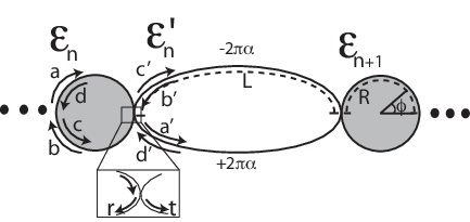
We assume the resonators have length and the total length of the connecting waveguides is , as shown in Fig.6. Therefore, transfer matrices corresponding to free propagation inside resonators and waveguides are:
respectively, where the wave number is and is the light frequency. We assume that the clockwise and counter-clockwise modes, i.e., forward and backward fields, are decoupled from each other, which sets the off-diagonal elements in and to be zero. The regime where this coupling between forward and backward fields becomes important is discussed in the main text and also in Sec.IV of this supplemental information (SI). We further assume that the coupling regions are long enough (compared to the wavelength of light) so that the coupling between clockwise and counter-clockwise photons (e.g. the coupling between and fields) can be ignored. In other words, a single coupling region couples only to and to . Therefore, a loss-less coupling region can be characterized by two parameters and , which represent the amount of transmission into and reflection off of the adjacent element, respectively, as shown in Fig.6. Note that these coefficients obeys the conditions: and . One can easily find the transfer matrix elements of such coupling regions for and , by setting and , and similarly for coupling between and . Therefore, the transfer matrix of a single coupling region which couples to and to can be written as:
In this notation, the field amplitudes in the right edge of the waveguide can be obtained from that of the adjacent resonator: .
The transfer matrix of the building block of such system () is a product of the above matrices . Using Bloch’s theorem, the dispersion relation is written as:
| (37) |
where is the Bloch quasi-momentum and is the unit spacing. First we solve the case where the phase imbalance between waveguide arms is zero (). We define the detuning from the resonator frequency as . We consider a configuration where resonators are separated by where is a non-zero integer and is the resonant wavelength. In this configuration, photon reflections off the resonators interfere destructively with each other, and therefore, photons spends most of their time in the resonators rather than the waveguides. We are primarily interested in relatively high quality factor resonators. Therefore, we evaluate the above expression to the first order in , which is proportional to the inverse of the resonators finesse . By assuming to be real and for resonators length, Eq.(37) gives a dispersion relation: , where characterizes the cavity field decay rate from on side of the resonator into the waveguides, i.e., the photon decay is . This decay is the extrinsic desirable decay, in contrast to intrinsic loss () which we discuss in Sec.V. Note that the sign of the tunneling amplitude depends on the parity of , which we assume to be odd ( in Fig.1a of the main text), so that we get the conventional minus sign in the tight-binding Hamiltonian.
Alternatively, one can also diagonalize the transfer matrix of a cell and study its eigenvalues as propagating waves. Under the above assumption, the diagonalized form of the transfer matrix of a unit cell will be of the following form:
| (38) |
We can infer: , which is equivalent to the aforementioned dispersion relation. Again, this shows that the propagating wave only exists when . Note that in this situation, we have two modes with the same dispersion relation, which corresponds to clockwise and counter-clockwise photons inside the resonators.
Furthermore, we consider the situation where there is a phase imbalance between waveguide arms. In this case, the diagonalized form of the transfer matrix takes the form:
| (39) |
From Eq.(37) one can easily see that the above transfer matrix corresponds to two dispersion relations: , which is the same dispersion of the tight-binding Hamiltonian in 1D with a magnetic field:
| (40) |
In particular, the mode corresponding to (c,d) fields in the resonators (pseudo-spin up) experiences a magnetic field () , while the mode corresponding to (a,d) field (pseudo-spin down) experiences an opposite magnetic field . In a 2D arrangement, by choosing these imbalances to be a function of rows , spin-up (spin-down) photons experience a uniform magnetic field corresponding to flux per plaquette, respectively.
II Derivation of the Hamiltonian with scatterers
In this section, we show that by implanting a scatterer in the system, one can achieve a photonic version of different quantum spin Hall Hamiltonians. In particular, the presence of a scatterer in each resonator leads to an effective “in-plane magnetic field” and the presence of scatterer in each connecting waveguides leads to a “spin-flip hopping” term. Below, we consider these effects.
II.1 Spin-flip hopping
Here, we study of the effect of scatterers in the connecting waveguides. In particular, we position two scatterers symmetrically in the middle of each waveguide, as shown in Fig.1(c) of the the main text. Therefore, the transfer matrix of the scatterer which couples (a,d) and (b,c) field together (as defined in Eq.18), is given by:
| (41) |
In this situation, the transfer matrix of the unit cell is given by:
| (42) |
We assume the scatterer is weak so we can write the transmission/reflection coefficients in the following form:
| (43) | |||||
| (44) |
In the absence of the scatterer, (a,b) and (c,d) modes couple to each other independently, i.e. couples to and couples to . As we discussed, these decoupled manifolds form an identical tight-biding Hamiltonian for two pseudo-spin components which we call (). However, the scatterer couples these two manifolds to each other. It turns out that a proper basis in the presence of the scatterer is a Hadamard rotated basis, i.e. and . This can be verified by using a degenerate perturbative method to find eigenvalues of the transfer matrix. Therefore, one finds out that the basis which diagonalizes M in the subspace of (a,c) or (b,d) is the x-basis –i.e. . The eigenvalues of the system to the zeroth order in inverse of resonator finesse ) are:
| (45) | |||||
| (46) |
These eigenstates have magnitude equal to one. Since each pair of eigenvalues are complex conjugate of each other, the four eigenvalues of system can be written in form of Bloch waves:
This leads to two dispersion relations to the first order in :
which can be simply written as:
Now, we want to write this Hamiltonian in the second quantized form using the original pseudo-spin components in z-basis (). Note that the above dispersion relation is written in the Hadamard rotated basis where . Therefore, we have:
| (47) |
The Hamiltonian in the original basis takes the conventional hopping flip term:
| (48) |
While the direct hopping amplitude is , the spin-flip hopping amplitude is . We note the above Hamiltonian is only valid when the scatters are positioned symmetrically in the middle of waveguides. If we move the scatterers symmetrically along the waveguides, we arrive at the same form of Hamiltonian with a modified strength of spin-flip term.
II.2 In-plane magnetic field
We now evaluate the effect of having a scatterer in every resonator rather than the waveguides. As we show, this model results in an in-plane magnetic field term in the Hamiltonian.
In this case the transfer matrix of the unit cell is: . Writing again the transfer matrix in the x-basis, we perturbatively find the eigenvalues to the zeroth order in and the first order in :
Therefore, the dispersion relations will be
The corresponding Hamiltonian in the x-basis is:
| (49) |
where the finesse of the resonators , characterizes the average number of photon round trip before leaving the resonator. The above Hamiltonian show that the scatterer inside the resonator lifts degeneracy and splits the modes. The splitting is proportional the strength of the scatterer and the number of photon round trips inside the resonator. In the original z-basis , the Hamiltonian takes the form:
| (50) |
This means that the presence of the scatterer inside the resonators result in an in-plane magnetic field. The amplitude of this in-plane magnetic field is given by the strength of the scatterer and the number of photon round trips inside the resonator. Similar to the spin-flip term, the strength of this terms can modified by symmetrically moving the scatterers long the resonators.
In the end, we note that the backscattering can also occur in the waveguides. However, in contrast to the resonator case, where the scattering was enhanced by the finesse of the resonators, the backscattering effect in the waveguides is not enhanced due the off-resonant nature of the waveguide loops.
III Input-Output formalism for probing the photonic system
We now consider the effects of coupling “probe” waveguides to the system. When the system and probe waveguides are not coupled to each other the Hamiltonian is given by The first term corresponds to the system which we want to probe and the the second term corresponds to free propagating light in the probing waveguide, i.e., where represents the state of one photon in the waveguide with wave number k. We note that since the system is linear and we are interested in the linear response, we treat the system in the first quantized representation and do not use creation and annihilation operators. On the other hand, the resonator fields are coupled to the forward- and backward-going field of the probing waveguides represented by the following coupling to the tight-binding Hamiltonian:
| (51) | |||||
() represents the photonic state of the resonator which is coupled to the input- (or output-) waveguide. We assume that resonators to be large enough so that each resonator mode couples to single running wave in the probing waveguides. For instance, CCW mode of the resonators is coupled to forward- (backward-) going light field at the input (output) probing waveguides, respectively (Fig.1(b) of the main text). Therefore, only positive (negative) momentum terms have non-zero coefficient in input (output) Hamiltonian terms. is the length of the waveguides which enters as a normalization factor.
Now, we want to study the scattering of an incoming plane wave which is sent into the probing waveguide. The effect of system-probe coupling is manifested in the output light field () which leaves the system in the probing waveguides. Since the system is linear, one can also look at this process from a single-photon picture: a photon comes from the input waveguide, while the system is initially in the vacuum state. Then, the photon interacts with system and eventually gets scattered into different output channels. The photon leaves through the probing waveguides and the system returns to original vacuum state.
In order to study such transport effects, we follow the formalism introduced in Refs.[27, 28] to investigate our system. We start by Lippmann-Schwinger equation:
| (52) |
which can be solved through iteration:
| (53) |
In other words, the T-matrix which characterizes the scattering amplitudes into different output channels can be written as:
| (54) |
Since the total system is linear, each photon should be exchanged an even number of times between the waveguide and the system to have a non-zero contribution in the output field. Therefore, only even powers in the above expression have non-zero contribution to the T-Matrix. In other words,
| (55) |
where the Green’s function is defined as: and is the uncoupled Green’s function of the system (probe), respectively. Indices (m,n) sums over different system eigenmodes, i.e., without the probing waveguides. The perturbative series can be summed to yield the exact Green’s function in the form:
| (56) |
where the self-energy of the coupled system is given by: We assume that the group velocity of the waveguide (in the absence of the coupling to the system) is smooth around the resonators frequency. In this limit, the interaction coefficient can be written as:
| (57) |
where is the coupling coefficient at the wave vector corresponding to the resonant frequency of the ring resonators (i.e. ). We transform the momentum sum of the self-energy expression into an integral. The real part of the integral corresponds to a constant energy shift which can be absorbed in the energy definition. The imaginary part of the self-energy corresponding to input channel is: , which shows that the field inside the input resonator will decay into the input waveguide at a rate , where is the group velocity at the resonator frequency. Similarly, one can evaluate the output self-energy terms. The self-energy for the total system can be written as
| (58) |
Note that the Green’s function in Eq.(56), can be also written as , which can be represented as a matrix and easily evaluated numerically.
Now, having the Green’s function of the coupled system, we return to the evaluation of the scattered field. We start by evaluating the wavefunction of the transmitted field in the same input channel (as shown in Fig.(1)b in the main text), which can be defined as and the input field is with . One can write the transmission coefficient in terms of the T-matrix: By using the T-matrix expression in Eq.(55), and the Green’s function, we can formally write the wavefunction of the transmitted field. The first term in the T-matrix gives the trivial unperturbed wavefunction . The second term can be written as:
Again by transforming the momentum sum into an integral and performing the contour integral, the pre-factor before the resonator summation simply reduces to . Therefore, the transmission coefficient for a given frequency will become:
| (59) |
Similarly, one can obtain the other transport coefficients:
IV Back-scattering disorders
The presence of scatterers in the system leads to mixing of pseudo-spin up and spin down, acting as a “magnetic disorder”. If this coupling is done in a controllable fashion, we arrive at the spin coupling Hamiltonians discussed earlier. However, in a experimental realization undesired backscatterings (e.g., due to surface roughness) lead to a similar coupling between spin-up and -down components. In most cases, this coupling is negligible. This has been the case for coupled resonators system [45, 46, 47, 48, 33]. However, in very high-Q resonators, the mode coupling (e.g., due to surface roughness) is usually greater than the resonator decay rate. In this case, the resonator enhances of the backscattering effect, and a mode splitting occurs [49, 50]. We note that as long as the interest is in the linear regime (as in this article), very high-Q resonators are not required. Nevertheless for completeness, we study the backscattering effect by first characterizing it and then evaluating its effects. As we show below, the effect of backscattering is more pronounced in the resonators and can be modeled by a magnetic disorder Hamiltonian. Before showing the derivation of the magnetic disorder Hamiltonian, we present the result of such model. In particular, we consider a case where at the resonator (), a scatterer is present and characterized by transmission (reflection) coefficient as (), respectively. The corresponding perturbation will be:
| (60) |
where depends on the position of the scatterer inside the resonator. The effect of such term can be understood in the following way: If we consider a forward-going spin-up wave, the disorder (to the first order in ) scatters the photon current into forward- and backward-going spin-down wave. Similar effects occur for other spin currents. This is in direct analogy to a “magnetic disorder” in the context of electronic QSHE, where electronic spin currents are not immune to magnetic impurities. Since our system is bosonic such impurities does not break the time reversal symmetry. However, their presence has a similar effect to magnetic impurities in fermionic QSHE. In particular, if we excite the system in spin-up modes, due to backscattering, spin-down modes will be also populated. However, since spin-up and -down are coupled to different output channels (i.e., and , respectively), the backscattering effect will be manifested in the reduction of signal in channels and some leakage in channels. Fig.4 in the main text shows different transport coefficients where we have assumed the backscattering is as strong as the dissipative loss. We observe that although the transport properties of magnetic bands states are affected by such magnetic impurities, edge state transport is robust, which is due the suppression of backscattering events. In particular, the scattering of a forward-going spin-up into forward (backward) -going spin-down is inhibited due to energy (momentum) mismatch.
Here we show that the effect of having an scatterer in a resonator can be modeled by a simple perturbation in our Hamiltonian formalism. The scatterer inside the resonator back-scatters the photon in the opposite mode, which in our spin language means that the spin-up photons can be scattered into spin down photons, vice verse. In particular, we consider the following scenario: a spin-up forward propagating photon current, in the presence of a back-scatterer in a resonator on its way, can get back-scattered into forward- and backward-going spin-down current (Fig.7). We first study this scenario in the physical system of a 1D array of resonators by transfer matrix formalism to evaluate the forward- and backward-going spin-down field amplitudes. Then, we study a model Hamiltonian and evaluate the scattered field amplitudes. By comparing the physical system and the model Hamiltonian, we argue that the physical system can be faithfully modeled by our proposed Hamiltonian.

First, we consider a 1D array of resonators and locate a disorder inside a single resonator and evaluate the transport properties of the a traveling spin wave off that disorder. In the absence of disorder the system possesses four modes, corresponding to clockwise and counter-clockwise modes of the resonators where each can propagate forwards or backwards. Therefore, at each site the photonic field can be represented by a 4 dimensional vector. We work in the basis of this four modes: so for example represents the forward spin-up photons and similarly for the three other modes.
In this basis, as discussed in the Sec.I of this SI, the transfer matrix of each cell is diagonalized in the following form:
| (61) |
where and . Now, we consider that there is a cell with a disorder located at site zero (). The propagation of a free travelling spin wave can be deduced by application of the transfer matrix ). In particular, we are interested in the reflected () and the transmitted field . However, these output field are not readily available in the transfer matrix, and we have to use the S-matrix. More precisely, , while for S-matrix: . In our case, we deal with two forward- and two backward-modes, so the M-matrix is characterized by 2x2 blocks as: , therefore, the corresponding S-matrix will be given by .
We consider a situation where the disorder is in the middle of the resonator in the upper arm. Therefore, the transfer matrix of two cells with a disorder in between will be . The corresponding S-matrix to the first order in the disorder strength () and the zeroth order in the inverse of the finesse (), will be:
| (62) |
where the first part simply represents the free propagation over two cells, and the second part represents the scattering into the other modes due backscattering. Note that as the scatterer is in the resonator, its strength is enhanced by the finesses of the resonator. Now, we consider a travelling spin-up wave which goes forward. For convenience, we assume the phase of this wave is such that it is zero at the site with the disorder. Therefore, our input will be: Since we are considering the propagation over two cells, in the absence of the scatterer, the output field should be: However, in the presence of the scatterer, we will have: The second (forth) row terms correspond to spin-down forward- (backward-) going amplitudes.
Now, we consider a tight-binding model with a disorder and show that it has the same behavior as our photonic system. In particular, we assume that the Hamiltonian of the system to be:
| (63) |
where the first term corresponds to a simple spin-conserving hopping Hamiltonian and the second terms corresponds to a magnetic disorder at site zero which rotates the pseudo-spin along the x-axis at the specific site. We assume the disorder to be weak (). Since the system is linear, the dynamics of the system can be studied by considering a single excitation. Therefore, a general state of the system can be captured in a two-component wavefunction as a function of sites: In particular, since we are interested in the scattering of a forward-going spin-up excitation off a disorder positioned at site m=0, the wavefunction of the entire system can be described as:
| (64) | |||||
| (65) | |||||
| (66) |
| (67) | |||||
| (68) | |||||
| (69) |
where (), corresponds to the transmitted amplitude of the spin-up (-down) component. Similarly, (), corresponds to the reflected amplitude of the spin-up (-down) component. Now, using the above ansatz, we solve the Schrodinger equation: , for and , which leads to seven independent equations:
| (70) | |||||
| (71) | |||||
| (72) | |||||
| (73) | |||||
| (74) | |||||
| (75) | |||||
| (76) |
We can solve the above equations for an arbitrary value of . However, since we are only interested in weak impurities, we present the solutions to the first order in :
| , | (77) | ||||
| (78) |
These results mean that a forward-going spin-up wave scatters into forward- and backward-going spin-down wave. This is identical to the perturbative result of our physical system (i.e. resonators and waveguides). In particular, if we set and , then the model Hamiltonian in Eq.60 and Eq. 63 are equivalent to each other and they describe the scattering inside the resonator. We note the the above derivations can be also reproduced for scattering of a spin-down wave propagating in the forward or backward direction.
Moreover, we note that where the scatterer is not positioned in the middle of the resonator the effective Hamiltonian is no longer an in-plane magnetic field in the x-direction. For a general position, the model Hamiltonian takes the form:
| (79) |
where the scattering terms corresponds to a magnetic field pointing in a random direction in the system plane.
Furthermore, we note that one might be tempted to try an educated guess based on the spin Hall Hamiltonian presented in Sec.II, without performing the above calculations. However, due the high symmetry of the system considered in Sec.II (symmetric positioning of the scatterers), we can not arrive at a rigorous approach to find the exact form and the coefficients of Eq.(63). In particular, varying the position of the scatterer in the single disorder case leads to a magnetic field pointing in any direction in the plane, while in the spin Hall model of Sec.II, symmetrically varying the position of the scatterers leads to only a strength modification of the in-plane magnetic field.
V Effect of loss
Here we discuss the effect of photonic loss which leads to leakage of photons out of the system. The loss can occur both in resonators and in the connecting waveguides. In most system, propagation and bending losses dominate the light attenuation and one can ignore losses due to coupling regions [51, 33]. We characterize the propagation loss and the bending loss at turns by a single quantity which is the field attenuation in a roundtrip inside the resonator. By assuming moderate quality factor for resonators and using transfer matrix formalism, one can easily show that the dispersion relation of a 1D array of resonators takes the form:
| (80) |
This loss can be also represented by a non-hermitian term in the Hamiltonian:
| (81) |
where the dissipation rate is given as the product of loss per roundtrip, number of roundtrips per decay time and the photon decay rate ().
Fig.4(c) of the main text shows the reflection spectrum in the presence of such loss. In the edge state transfer band, the reflection is slightly attenuated due to the attenuation of the light field during the propagation around the system perimeter . We note that the numerical results corroborate with this estimate.
VI Experimental considerations
We next consider experimental issues involving the realization and detection of the magnetic photonic states. Although our formalism is general and can be applied to various photonic systems, here, we focus on silicon-on-insulator (SOI) technology where it has been shown that up to 100 micro-ring resonators can be successfully coupled to each other operating at 1.5 [33]. We consider a 10x10 lattice and take the unit cell as 20. Since for a typical ring of a few microns, bending losses (dB/turn) are typically larger than propagation losses over a wavelength (dB/cm)[51, 33], using waveguides with different lengths to connect the resonators might be experimentally more accessible than coupling rings as in a Mach-Zender configuration [24, 25]. Using the experimental parameter in Ref. [33], we find that the extrinsic decay is , which is half of the bandwidth of the tight-binding model. The intrinsic loss is and the standard deviation of individual resonances is . In numerical simulations for Fig.4 and 5 of the main text, we use these parameters and assume that the backscattering strength is .