How to transform and filter images using iterated function systems.

Michael F. Barnsley ^†^†thanks: Department of Mathematics Australian National University Canberra, ACT, Australia (michael.barnsley@math.anu.edu.au). Brendan Harding ^†^†thanks: Department of Mathematics, Australian National University (brendan.harding@anu.edu.au). Konstantin Igudesman ^†^†thanks: Faculty of Mechanics and Mathematics Kazan State University Kazan, Russian Federation (kigudesm@yandex.ru).

Abstract

We present a general theory of fractal transformations and show how it leads to new type of method for filtering and transforming digital images. This work substantially generalizes earlier work on fractal tops. The approach involves fractal geometry, chaotic dynamics, and an interplay between discrete and continuous representations. The underlying mathematics is established and applications to digital imaging are described and exemplified.

keywords

Iterated function systems, dynamical systems, fractal transformations.

AMS

37B10, 54H20, 68U10

1 Introduction

Fractal transformations are mappings between pairs of attractors of iterated function systems. They are defined with the aid of code space structures, and can be quite simple to handle and compute. They can be applied to digital images when the attractors are rectangular subsets of $\mathbb{R}^{2}$ . They are termed ”fractal” because they can change the box-counting, Hausdorff, and other dimensions of sets and measures upon which they act. In this paper we substantially generalize and develop the theory and we illustrate how it may be applied to digital imaging. Previous work was restricted to fractal transformations defined using fractal tops.

Fractal tops were introduced in [2] and further developed in [5, 6, 7, 11]. The main idea is this: given an iterated function system with a coding map and an attractor, a section of the coding map, called a tops function, can be defined using the ”top” addresses of points on the attractor. Given two iterated function systems each with an attractor, a coding map, and a common code space, a mapping from one attractor to the other can be constructed by composing the tops function, for the first iterated function system, with the coding map for the second system. Under various conditions the composed map, from one attractor to the other, is continuous or a homeomorphism. In the cases of affine and projective iterated function systems, practical methods based on the chaos game algorithm [8] are feasible for the approximate digital computation of such transformations. Fractal tops have applications to information theory and to computer graphics. They have been applied to the production of artwork, as discussed for example in [4], and to real-time image synthesis [18]. In the present paper we extend the theory and applications.

Much of the material in this paper is new. The underlying new idea is that diverse sections of a coding map may be defined quite generally, but specifically enough to be useful, by associating certain dynamical systems with the iterated function system. These sections provide novel collections of fractal transformations; by their means we generalize the theory and applications of fractal tops. We establish properties of fractal transformations, including conditions under which they are continuous. The properties are illustrated by examples related to digital imaging.

A notable result, Theorem 21, states the existence of nontrivial fractal homeomorphisms between attractors of some affine overlapping iterated function systems. The proof explains how to construct them. An example of one of these new homeomorphisms, applied to a picture of Lena, is illustrated in Figure 1.

Refer to caption — Fig. 1: Lena after application of a fractal homeomorphism. See Example 23.

In Section 2 we review briefly the key definitions and results concerning point-fibred iterated function systems on compact Hausdorff spaces. Since this material is not well-known, it is of independent interest. The main result is Theorem 4. This can be viewed as a restatement of some ideas in [13]; it describes the relationship between the coding map and the attractor of a point-fibred iterated function system.

In Section 3 we define, and establish some general properties of, fractal transformations constructed using sections of coding maps. In Theorem 8 we present some general properties of coding maps. Then we use coding maps to define fractal transformations and, in Theorem 10, we provide sufficient conditions for a fractal transformation to be continuous or homeomorphic.

In Section 4 we define two different types of section of a coding map: (i) with the aid of a masked dynamical system; and (ii) with the aid of fractal tops. Theorem 14 establishes the connection between the masked dynamical system and a masked section of the coding map. Theorem 16 includes a statement concerning the relationship between the masked section to the coding map and the shift map. Here we also establish the relationship between fractal tops and masked systems. A key result, Theorem 18, gives a condition under which the ranges of different masked sections intersect in a set of measure zero. This enables the approximate storage of multiple images in a single image, as illustrated in Figure 9.

In Section 5 we apply and illustrate the theoretical structures of Sections 2,3, and 4, in the context of digital imaging. Our goal is to illustate the diversity of imaging techniques that are made feasible by our techniques, and to suggest that fractal transformations have a potentially valuable role to play in digital imaging. In Section 5.1 we illustrate how fractal transformations may be applied to image synthesis, that is to making artificial interesting and even beautiful pictures. Specifically we explain how the technique of color-stealing [2] extends to masked systems. In Section 5.2 we apply fractal homeomorphisms, using Theorem 10, to transform digital images, for image beautification, roughening, and special effects; in particular, we present and illustrate Theorem 21 which extends the set of known affine fractal homeomophisms. In Section 5.3 we consider the idea of composing a fractal transformation, discretization, and the inverse of the transformation to make idempotent image filters. In Section 5.4 we apply Theorem 18 to the approximate storage or encryption of multiple images in a single image. In Section 5.5 we provide a second technique for combining several images in one: it combines invariant measures of a single iterated function system with several sets of probabilities, to make a single ”encoded” image: approximations to the original images are revealed by the application of several fractal homeomorphisms.

2 Point-fibred iterated function systems

Let $X$ be a nonempty compact Hausdorff space, and let $K(X)$ be the set of nonempty compact subsets of $X$ . It is known that $K(X)$ endowed with the Vietoris topology is a compact Hausdorff space, see for example [14, Theorem 2.3.5, p.17]. This encompasses the well-known fact that if $X$ is a compact metric space then $K(X)$ endowed with the Hausdorff metric is a compact metric space. Let $I=\left\{1,2,...N\right\}$ be a finite index set with the discrete topology. Let $\left\{f_{i}:X\rightarrow X|i\in I\right\}$ be a sequence of continuous functions. Following [2],

\mathcal{F}:=(X;f_{1},\ldots f_{N})

is called an iterated function system over $X$ .

Following [13, Definition 4.1.4, p.84] we define a map

\Pi:I^{\infty}\rightarrow K(X),\text{ }\sigma\mapsto\bigcap\limits_{k=1}^{\infty}f_{\sigma_{1}}\circ f_{\sigma_{2}}\circ\cdots\circ f_{\sigma_{k}}(X)

(1)

for all sequences $\sigma=\sigma_{1}\sigma_{2}\sigma_{3}...$ belonging to $I^{\infty}$ . The map is well-defined because $\Pi(\sigma)$ is the intersection of a nested sequence of nonempty compact sets. The following definition is based on [13, Definition 4.3.6, p.97].

Definition 1.

Let $\mathcal{F}:=(X;f_{1},\ldots f_{N})$ be an iterated function system over a compact Hausdorff space $X$ . If $\Pi(\sigma)$ is a singleton for all $\sigma\in I^{\infty}$ then $\mathcal{F}$ is said to be point-fibred, and the coding map of $\mathcal{F}$ is defined by

\pi:I^{\infty}\rightarrow A\text{, }\left\{\pi(\sigma)\right\}=\Pi(\sigma),

where $A\subset X$ denotes the range of $\pi$ .

Theorem 2, due to Kieninger, plays a central role in this paper. It generalizes a classical result of Hutchinson [10] that applies when $X$ is a compact metric space and each $f\in\mathcal{F}$ is a contraction.

Theorem 2.

Let $I^{\infty}$ have the product topology. If $\mathcal{F}$ is a point-fibred iterated function system on a compact Hausdorff space $X$ then the coding map $\pi:I^{\infty}\rightarrow A$ is continuous.

Proof.

This follows from [13, Proposition 4.3.22, p.105]. ∎

We define

\mathcal{F}:K(X)\rightarrow K(X)\text{, }B\mapsto\bigcup_{f\in\mathcal{F}}f(B)\text{.}

By slight abuse of notation we use the same symbol $\mathcal{F}$ for the iterated function system, the maps that it comprises, and the latter function. We define $\mathcal{F}^{0}=i_{X}$ , the identity map on $X$ , and $\mathcal{F}^{k}=\mathcal{F}\circ\mathcal{F}^{k-1}$ for $k=1,2,...$ . The following definition is a natural generalization of the notion of an attractor of a contractive iterated function system, see for example [15, definition on p.1193 and Theorem 11.1, p.1206], [13, p.107], and also [8].

Definition 3.

Let $\mathcal{F}$ be an iterated function system on a compact Hausdorff space $X$ . An attractor of $\mathcal{F}$ is $A\in$ $K(X)$ with these properties: (i) $\mathcal{F}(A)=A$ ; (ii) there exists an open set $U\subset X$ such that $A\subset U$ and

\lim_{k\rightarrow\infty}\mathcal{F}^{k}(B)=A

(2)

for all $B\subset U$ with $B\in K(X)$ . (The limit is with respect to the Vietoris topology on $K(X)$ .) The largest open set $\mathcal{B}\subset X$ such that equation 2 holds for all $B\subset\mathcal{B}$ with $B\in K(X)$ is called the basin of $A$ .

The relationship between coding maps and attractors is provided by noting that

\pi(\sigma)=\lim_{k\rightarrow\infty}f_{\sigma|k}(a)\text{ where }f_{\sigma|k}:=f_{\sigma_{1}}\circ f_{\sigma_{2}}\circ\cdots\circ f_{\sigma_{k}}

for $a\in X$ . This leads to the following theorem.

Theorem 4.

If $\mathcal{F}$ is a point-fibred iterated function system on a compact Hausdorff space $X$ then

(i) $\mathcal{F}:K(X)\rightarrow K(X)$ has a unique fixed-point $A\in K(X),$ i.e. $\mathcal{F}\left(A\right)=A$ ;

(ii) $A$ is the unique attractor of $\mathcal{F}$ ;

(iii) $A$ is equal to the range of the coding map $\pi$ , namely

A=\pi(I^{\infty})\text{;}

(iv) the basin of $A$ is $X;$

(v) if $B\in K(X)$ then $\left\{\pi(\sigma)\right\}=\lim_{k\rightarrow\infty}f_{\sigma|k}(B)$ for all $\sigma\in I^{\infty}.$

Proof.

This follows from [13, Proposition 4.4.2, p.107, see also Proposition 3.4.4, p.77]. ∎

The following remark tells us that if an iterated function system possesses an attractor then it is point-fibred when restricted to a certain neighborhood of the attractor. Necessary and sufficient conditions for an iterated function system of projective transformations to possess an attractor are given in [9].

Remark 5.

Let $A$ be an attractor of an iterated function system $\mathcal{F}$ on a compact Hausdorff space $X$ , and let $\mathcal{B}$ be the basin of $A.$ Then, following [15], $\mathcal{F}$ defines an iterated closed relation $r:=\{(x,f(x)):x\in X,f\in\mathcal{F}\}\subset X\times X$ , and $A$ is an attractor of $r$ . By [15, Theorem 7.2, p.1193] there exists a compact neighborhood $V$ of $A$ such that $A\subset Int_{X}(V)$ and $\mathcal{F}\left(V\right)\subset Int_{X}(V).$ ( $Int_{X}(S)$ denotes the interior of the set $S\subset X$ in the subspace topology induced on $S$ by $X$ .) It follows that $\mathcal{F}|_{V}:=(V;f_{1}|_{V},f_{2}|_{V},...f_{N}|_{V})$ is a point-fibred iterated function system on a compact Hausdorff space. The attractor of $\mathcal{F}|_{V}$ is $A.$

Definition 6.

Let $\mathcal{F}$ be a point-fibred iterated function system on a compact Hausdorff space. The set $I^{\infty}$ is called the code space of $\mathcal{F}$ . A point $\sigma\in I^{\infty}$ is called an address of $\pi(\sigma)\in A$ .

In the rest of this paper the underlying space $X$ is a compact Hausdorff space. Also in the rest of this paper the symbols $\mathcal{F},\mathcal{G},\mathcal{H}$ denote point-fibred iterated function systems on compact Hausdorff spaces. We will say that an iterated function system is injective when all of the maps that it comprises are injective. We will say that an iterated function system is open when all of the maps that it comprises are open.

3 Fractal transformations

Here we present a generalized theory of fractal transformations and establish some continuity properties. Fractal transformations are defined using sections of coding maps. We are concerned with continuity properties; for example, Theorem 10 (i) provides a sufficient condition for a fractal transformation to be continuous.

Definition 7.

Let $\pi:I^{\infty}\rightarrow A$ be the coding map of $\mathcal{F}$ . A subset $\Omega\subset I^{\infty}$ is called an address space for $\mathcal{F}$ if $\pi(\Omega)=A$ and $\pi|_{\Omega}:\Omega\rightarrow A\subset X$ is one-to-one. The corresponding map

\tau:A\rightarrow\Omega,x\mapsto(\pi|_{\Omega})^{-1}(x)\text{,}

is called a section of $\pi$ .

Theorem 8 summarises the properties of sections of $\pi.$

Theorem 8.

Let $\mathcal{F}=(X;f_{1},f_{2},...,f_{N})$ be a point-fibred iterated function system on a compact Hausdorff space, with attractor $A$ , code space $I^{\infty}$ , and coding map $\pi:I^{\infty}\rightarrow A.$ If $\tau:A\rightarrow\Omega$ is a section of $\pi$ then

(i) $\tau:A\rightarrow\Omega$ is bijective;

(ii) $\tau^{-1}:\Omega\rightarrow$ $A$ is continuous;

(iii) $\pi\circ\tau=\iota_{A}$ , the identity map on $A,$ and $\tau\circ\left(\pi|_{\Omega}\right)=\iota_{\Omega}$ , the identity map on $\Omega$ ;

(iv) if $\mathcal{F}$ is injective and $f_{i}(A)\cap f_{j}(A)=\emptyset$ for all $\ i,j\in I$ with $i\neq j$ , then $\Omega=I^{\infty}$ ;

(v) if $\Omega$ is closed then $\tau:A\rightarrow\Omega$ is a homeomorphism;

(vi) if $A$ is connected and $A$ is not a singleton, then $\tau:A\rightarrow\Omega$ is not continuous.

Proof.

(i) By Definition 7 $\pi|_{\Omega}:\Omega\rightarrow A$ is bijective, so $\tau=$ $(\pi|_{\Omega})^{-1}:A\rightarrow\Omega$ is bijective.

(ii) By Theorem 2 $\pi:I^{\infty}\rightarrow A$ is continuous. It follows that $\tau^{-1}=\pi|_{\Omega}:\Omega\rightarrow A$ is continuous.

(iii) If $x\in A$ then $\pi\circ\tau(x)=\pi\circ\left(\pi|_{\Omega}\right)^{-1}(x)\subset\pi\circ\pi^{-1}(x)=x=i_{A}(x).$ Also $\tau\circ\pi|_{\Omega}=\tau\circ\tau^{-1}=\iota_{\Omega}$ .

(iv) Suppose $\Omega\neq I^{\infty}$ . Then there are $\sigma,\omega\in I^{\infty}$ , $\sigma\neq\omega$ , such that $\pi(\sigma)=\pi(\omega)$ . We show that this is impossible. If $\pi(\sigma)=\pi(\omega)$ then Theorem 4 (v) implies $\left\{\pi(\sigma)\right\}=\lim_{k\rightarrow\infty}f_{\sigma|k}(A)=\lim_{k\rightarrow\infty}f_{\omega|k}(A)=\left\{\pi(\omega)\right\}$ . Let $K$ be the least integer such that $\omega_{K+1}\neq\sigma_{K+1}$ . Then $f_{\omega|K}=f_{\sigma|K}$ and $f_{\omega_{K+1}}(A)\cap f_{\sigma_{K+1}}(A)=\emptyset$ . Since $\mathcal{F}$ is injective, each $f\in\mathcal{F}$ is injective, which implies that $f_{\omega|K}:X\rightarrow X$ is injective. Since $f_{\omega|K}=f_{\sigma|K}$ , it now follows that $f_{\omega|K+1}(A)\cap f_{\sigma|K+1}(A)=f_{\omega|K}(f_{\omega_{K+1}}\left(A\right))\cap f_{\sigma|K}(f_{\sigma_{K+1}}\left(A\right))=f_{\omega|K}(f_{\sigma_{K+1}}\left(A\right))\cap f_{\omega|K}(f_{\omega_{K+1}}\left(A\right))=\emptyset$ . Since $\left\{\pi(\sigma)\right\}\subset f_{\sigma|K+1}(A)$ and $\left\{\pi(\omega)\right\}\subset f_{\omega|K+1}(A)$ it now follows that $\left\{\pi(\sigma)\right\}\cap\left\{\pi(\omega)\right\}=\emptyset$ .

(v) If $\Omega\subset I^{\infty}$ is closed then it is compact, because $I^{\infty}$ is compact. It follows that $\tau^{-1}=\pi|_{\Omega}:\Omega\rightarrow A$ is a continuous bijective mapping from a compact space $\Omega$ onto a Hausdorff space $A$ . By [17, Theorem 5.6, p.167] it follows that $\tau^{-1}:\Omega\rightarrow A$ is a homeomorphism. It follows that $\tau:A\rightarrow\Omega$ is a homeomorphism.

(vi) Suppose that $A$ is connected and $A$ is not a singleton. It follows that $\Omega$ is not a singleton. It follows that $\Omega$ is not connected. (Since $\Omega$ contains more than one point and is a subset of $I^{\infty},$ which is totally disconnected when it contains more than one point, it follows that $\Omega$ is not connected.)

Now suppose $\tau:A\rightarrow\Omega$ is continuous. Then $\tau$ is a homeomorphism. It follows that $A$ is not connected. But $A$ is connected. So $\tau:A\rightarrow\Omega$ is not continuous. ∎

In Definition 9 we define a type of transformation between attractors of iterated function systems by composing sections of coding maps with coding maps. We call these transformations ”fractal” because they can be very rough; specific examples demonstrate that the graphs of these transformations, between compact manifolds, can possess a non-integer Hausdorff-Besicovitch dimension.

Definition 9.

Let $\mathcal{F}=(X;f_{1},f_{2},...,f_{N})$ be a point-fibred iterated function system over a compact Hausdorff space $X$ . Let $A_{\mathcal{F}}\subset X$ be the attractor of $\mathcal{F}$ . Let $\pi_{\mathcal{F}}:I^{\infty}\rightarrow A_{\mathcal{F}}$ be the coding map of $\mathcal{F}$ . Let $\tau_{\mathcal{F}}:A_{\mathcal{F}}\rightarrow\Omega_{\mathcal{F}}\subset I^{\infty}$ be a branch of $\pi_{\mathcal{F}}$ . Let $\mathcal{G}=(Y;g_{1},g_{2},...,g_{N})$ be a point-fibred iterated function system over a compact Hausdorff space $Y.$ Let $A_{\mathcal{G}}$ be the attractor of $\mathcal{G}$ . Let $\pi_{\mathcal{G}}:I^{\infty}\rightarrow A_{\mathcal{G}}$ be the coding map of $\mathcal{G}$ . The corresponding fractal transformation is defined to be

T_{\mathcal{FG}}:A_{\mathcal{F}}\rightarrow A_{\mathcal{G}}\text{, }x\longmapsto\pi_{\mathcal{G}}\circ\tau_{\mathcal{F}}(x)\text{.}

In Theorem 10 we describe some continuity properties of fractal transformations. These properties make fractal transformations interesting for applications to digital imaging.

Theorem 10.

Let $\mathcal{F}$ and $\mathcal{G}$ be point-fibred iterated function systems as in Definition 9. Let $T_{\mathcal{FG}}=\pi_{\mathcal{G}}\circ\tau_{\mathcal{F}}:A_{\mathcal{F}}\rightarrow A_{\mathcal{G}}$ be the corresponding fractal transformation.

(i) If, whenever $\sigma,\omega\in\overline{\Omega_{\mathcal{F}}}$ , $\pi_{\mathcal{F}}(\sigma)=\pi_{\mathcal{F}}(\omega)$ $\Rightarrow$ $\pi_{\mathcal{G}}(\sigma)=\pi_{\mathcal{G}}(\omega),$ then $T_{\mathcal{FG}}:A_{\mathcal{F}}\rightarrow A_{\mathcal{G}}$ is continuous.

(ii) If $\Omega_{\mathcal{G}}:=\Omega_{\mathcal{F}}$ is an address space for $\mathcal{G}$ , and if, whenever $\sigma,\omega\in\overline{\Omega_{\mathcal{F}}}$ , $\pi_{\mathcal{F}}(\sigma)=\pi_{\mathcal{F}}(\omega)$ $\Longleftrightarrow$ $\pi_{\mathcal{G}}(\sigma)=\pi_{\mathcal{G}}(\omega),$ then $T_{\mathcal{FG}}$ is a homeomorphism and $T_{\mathcal{FG}}^{-1}=T_{\mathcal{GF}}$ .

Proof.

(i) Assume that, whenever $\sigma,\omega\in\overline{\Omega_{\mathcal{F}}}$ , $\pi_{\mathcal{F}}(\sigma)=\pi_{\mathcal{F}}(\omega)$ $\Rightarrow$ $\pi_{\mathcal{G}}(\sigma)=\pi_{\mathcal{G}}(\omega)$ . We begin by showing that $\pi_{\mathcal{G}}\circ\tau_{\mathcal{F}}\circ\pi_{\mathcal{F}}|_{\overline{\Omega_{\mathcal{F}}}}:\overline{\Omega_{\mathcal{F}}}\rightarrow A_{\mathcal{G}}$ is the same as $\pi_{\mathcal{G}}|_{\overline{\Omega_{\mathcal{F}}}}:\overline{\Omega_{\mathcal{F}}}\rightarrow A_{\mathcal{G}}.$ Let $\sigma\in\overline{\Omega_{\mathcal{F}}}$ . Then there is $\omega\in\Omega_{\mathcal{F}}$ such that $\pi_{\mathcal{F}}(\sigma)=\pi_{\mathcal{F}}(\omega)$ because $\Omega_{\mathcal{F}}$ is a code space for $\mathcal{F}.$ Hence $\tau_{\mathcal{F}}\circ\pi_{\mathcal{F}}|_{\overline{\Omega_{\mathcal{F}}}}(\sigma)=\tau_{\mathcal{F}}\circ\pi_{\mathcal{F}}|_{\Omega_{\mathcal{F}}}(\omega)=\omega$ (using Theorem 8 (iii)). Hence $\pi_{\mathcal{G}}\circ\tau_{\mathcal{F}}\circ\pi_{\mathcal{F}}|_{\overline{\Omega_{\mathcal{F}}}}(\sigma)=\pi_{\mathcal{G}}(\omega)=\pi_{\mathcal{G}}(\sigma)$ , where we have used our initial assumption. It follows that $\pi_{\mathcal{G}}\circ\tau_{\mathcal{F}}\circ\pi_{\mathcal{F}}|_{\overline{\Omega_{\mathcal{F}}}}=\pi_{\mathcal{G}}|_{\overline{\Omega_{\mathcal{F}}}}$ . It follows that $\pi_{\mathcal{G}}\circ\tau_{\mathcal{F}}\circ\pi_{\mathcal{F}}|_{\overline{\Omega_{\mathcal{F}}}}$ is a continuous map from a compact space $\overline{\Omega_{\mathcal{F}}}$ to a compact Hausdorff space $A_{\mathcal{G}}.$ But $\pi_{\mathcal{G}}\circ\tau_{\mathcal{F}}\circ\pi_{\mathcal{F}}|_{\overline{\Omega_{\mathcal{F}}}}=\left(\pi_{\mathcal{G}}\circ\tau_{\mathcal{F}}\right)\circ\pi_{\mathcal{F}}|_{\overline{\Omega_{\mathcal{F}}}}$ is the composition of a continuous mapping $\pi_{\mathcal{F}}|_{\overline{\Omega_{\mathcal{F}}}}:\overline{\Omega_{\mathcal{F}}}\rightarrow A_{\mathcal{F}},$ from a compact Hausdorff space $\overline{\Omega_{\mathcal{F}}}$ onto a Hausdorff space $A_{\mathcal{F}}$ , with a mapping $\pi_{\mathcal{G}}\circ\tau_{\mathcal{F}}:A_{\mathcal{F}}\rightarrow A_{\mathcal{G}}$ from $A_{\mathcal{F}}$ into a Hausdorff space $A_{\mathcal{G}}$ . It follows by a well-known theorem in topology, see for example [16, Proposition 7.4, p. 195], that $T_{\mathcal{FG}}=$ $\pi_{\mathcal{G}}\circ\tau_{\mathcal{F}}:A_{\mathcal{F}}\rightarrow A_{\mathcal{G}}$ is continuous.

(ii) Assume that $\Omega_{\mathcal{G}}=\Omega_{\mathcal{F}}$ is an address space for $\mathcal{G}$ , and that, whenever $\sigma,\omega\in\overline{\Omega_{\mathcal{F}}}$ , $\pi_{\mathcal{F}}(\sigma)=\pi_{\mathcal{F}}(\omega)$ $\Longleftrightarrow$ $\pi_{\mathcal{G}}(\sigma)=\pi_{\mathcal{G}}(\omega)$ . Then by (i) both of the mappings $T_{\mathcal{FG}}=\pi_{\mathcal{G}}\circ\tau_{\mathcal{F}}:A_{\mathcal{F}}\rightarrow A_{\mathcal{G}}$ and $T_{\mathcal{GF}}=\pi_{\mathcal{F}}\circ\tau_{\mathcal{G}}:A_{\mathcal{G}}\rightarrow A_{\mathcal{F}}$ are continuous. Using the fact that the range of $\tau_{\mathcal{G}}$ is $\Omega_{\mathcal{F}}$ it is readily checked that $T_{\mathcal{FG}}\circ T_{\mathcal{GF}}=\pi_{\mathcal{G}}\circ\tau_{\mathcal{F}}\circ$ $\pi_{\mathcal{F}}\circ\tau_{\mathcal{G}}=i_{A_{\mathcal{G}}}$ and $T_{\mathcal{GF}}\circ T_{\mathcal{FG}}=\pi_{\mathcal{F}}\circ\tau_{\mathcal{G}}\circ$ $\pi_{\mathcal{G}}\circ\tau_{\mathcal{F}}=i_{A_{\mathcal{F}}}.$ Hence $T_{\mathcal{FG}}$ is a homeomorphism and $T_{\mathcal{GF}}=\left(T_{\mathcal{FG}}\right)^{-1}$ . ∎

Remark 11.

Suppose that the equivalence relations $\sim_{\mathcal{F}}$ and $\sim_{\mathcal{G}}$ on $I^{\infty}$ , induced by $\pi_{\mathcal{F}}:I^{\infty}\rightarrow A_{\mathcal{G}}$ and $\pi_{\mathcal{G}}:I^{\infty}\rightarrow A_{\mathcal{G}}$ respectively, are the same. Then it is well known that, using compactness, the quotient topological space $I^{\infty}/\sim_{\mathcal{F}}=I^{\infty}/\sim_{\mathcal{G}}$ is homeomorphic to both $A_{\mathcal{F}}$ and $A_{\mathcal{G}}$ .

See [1] for discussion of relationships between the topology of an attractor and the equivalence class structure induced by a coding map.

4 Construction of sections of $\pi$

In order to construct a fractal transformation we need to specify a section of $\pi$ . In order to construct a section of $\pi$ we have to construct an address space $\Omega$ ; that is, we need to specify one element from each of the sets in the collection $\{\pi^{-1}(x):x\in A\}$ . To do this in a general way seems to be difficult; for example, if $f_{1}(A)\cap f_{2}(A)$ contains a nonempty open set $O$ , then $\pi^{-1}(x)$ is non-denumerable for all $x\in O$ . However there are two particular related methods. These methods yield interesting structure; for example, in both cases the resulting address space $\Omega\subset I^{\infty}$ is mapped into itself by the shift operator, see Theorem 16 (ii). They are as follows.

(a) (Masked iterated function system method.) This method requires that $\mathcal{F}$ is injective. Define a dynamical system on $T:A_{\mathcal{F}}\rightarrow A_{\mathcal{F}}$ with the aid of inverses of the functions in $\mathcal{F}$ . Follow orbits of $T$ to define $\tau_{\mathcal{F}}:A_{\mathcal{F}}\rightarrow\Omega_{\mathcal{F}}$ ; in effect one uses a Markov partition associated with $T$ to define $\Omega_{\mathcal{F}}$ .

(b) (Fractal tops method.) Use the dictionary order relation on $I^{\infty}$ to select a unique element of $\pi^{-1}(x)$ for each $x\in A_{\mathcal{F}}$ . This method applies when $\mathcal{F}$ is not required to be injective. When $\mathcal{F}$ is injective, it is a special case of (a). To date, the fractal tops method seems to be the easiest to convert to computational algorithms and applications.

4.1 (a) The masked iterated function system method

Definition 12 introduces a special partition of an attractor.

Definition 12.

Let $\mathcal{F}$ be a point-fibred iterated function system on a compact Hausdorff space. Let $A$ be the attractor of $\mathcal{F}$ . A finite sequence of sets $\mathcal{M}:=\{M_{i}\subset A|i\in I\}$ is called a mask for $\mathcal{F}$ if

1.

$M_{i}\subseteq f_{i}(A)$ , $i\in I$ ;
2.

$M_{i}\cap M_{j}=\emptyset$ , $i,j\in I$ , $i\neq j$ ;
3.

$\cup_{i\in I}M_{i}=A$ .

Note that for any $x\in A$ there exists a unique $i\in I$ such that $x\in M_{i}\subseteq f_{i}(A)$ . This enable us, in Definition 13, to define an associated dynamical system on the attractor.

Definition 13.

Let $\left\{M_{i}:i\in I\right\}$ be a mask for an injective point-fibred iterated function system $\mathcal{F}$ with attractor $A.$ The associated masked dynamical system for $\mathcal{F}$ is

T:A\rightarrow A,\quad x\mapsto\begin{cases}f_{1}^{-1}(x),&x\in M_{1},\\ f_{2}^{-1}(x),&x\in M_{2},\\ \qquad\vdots&\\ f_{N}^{-1}(x),&x\in M_{N}.\end{cases}

Theorem 14 associates a unique section of $\pi$ with a masked dynamical system.

Theorem 14.

Let $\mathcal{F}$ be an injective point-fibred iterated function system with attractor $A.$ Let $T:A\rightarrow A$ be a masked dynamical system for $\mathcal{F}$ , associated with mask $\mathcal{M}=\left\{M_{i}:i\in I\right\}$ . Let $x\in A$ and let $\left\{x_{n}\right\}_{n=0}^{\infty}$ be the orbit of $x$ under $T$ ; that is, $x_{0}=x$ and $x_{n}=T^{n}(x_{0})$ for $n=1,2,...$ . Let $\sigma_{k}(x)\in I$ be the unique symbol such that $x_{k-1}\in M_{\sigma_{k}}$ , for $k=1,2,3,...$ . Then

\Omega_{\mathcal{M}}=\{\sigma\in I^{\infty}|\sigma:=\sigma(x)=\sigma_{1}(x)\sigma_{2}(x)\sigma_{3}(x)...\in I^{\infty},x\in A\}

is an address space for $\mathcal{F}$ .

Proof.

Let $x\in A$ . We begin by proving that, for all $K\geq 1$ and $j=1,2,...,K-1,$ we have

x_{K-j}\in f_{\sigma_{K-j+1}(x)}f_{\sigma_{K-j+1}(x)}\circ...\circ f_{\sigma_{K}(x)}(A).

(3)

Fix $K.$ We use induction on $j.$ Since $x_{K-1}\in M_{\sigma_{K}}$ it follows that $x_{K}=f_{\sigma_{K}}^{-1}(x_{K-1})$ so $x_{K-1}=f_{\sigma_{K}(x)}(x_{K})\in f_{\sigma_{K}}(A)$ . It follows that equation 3 is true for $j=1$ . Suppose that equation 3 is true for $j=1,2,...,J\leq K-2$ . It follows that $x_{K-J}\in f_{\sigma_{K-J+1}(x)}\circ f_{\sigma_{K-J+1}(x)}\circ...\circ f_{\sigma_{K}(x)}(A)$ . We also have $x_{K-J}\in M_{\sigma_{K-J+1}}$ so $x_{K-J}=f_{\sigma_{K-J}}^{-1}(x_{K-J-1})$ which implies $x_{K-J-1}=f_{\sigma_{K-J}}(x_{K-J})\in f_{\sigma_{K-J(x)}}\left(f_{\sigma_{K-J+1}(x)}\circ f_{\sigma_{K-J+1}(x)}\circ...\circ f_{\sigma_{K}(x)}(A)\right).$ Hence equation 3 is true for $j=J+1$ . This completes the induction on $j$ .

It follows that

x=x_{0}\in f_{\sigma_{1}(x)}\circ f_{\sigma_{2}(x)}\circ...\circ f_{\sigma_{K}(x)}(A)

for all $K.$ It follows that $x\in\cap_{k=1}^{\infty}f_{\sigma_{1}(x)}\circ f_{\sigma_{2}(x)}\circ...\circ f_{\sigma_{k}(x)}(A)=\pi(\sigma(x))$ . It follows that $x=\pi(\sigma(x))$ for all $x\in A.$ It follows that $\pi|_{\Omega_{\mathcal{M}}}(\Omega_{\mathcal{M}})=A$ ; that is, $\pi|_{\Omega_{\mathcal{M}}}:\Omega_{\mathcal{M}}\rightarrow A$ is surjective.

To show that $\pi|_{\Omega_{\mathcal{M}}}:\Omega_{\mathcal{M}}\rightarrow A$ is injective, suppose $\sigma(x)\neq\sigma(y)\in\Omega_{\mathcal{M}}$ for some $x,y\in A.$ Then for some $k$ we have $\sigma(x)_{k}\neq\sigma(y)_{k}$ which implies $M_{\sigma(x)_{k}}\cap M_{\sigma(y)_{k}}=\emptyset$ . Hence $T^{k}(x)\neq T^{k}(y).$ It follows that $x\neq y$ . ∎

Definition 15.

Let $\mathcal{F}$ be an injective point-fibred iterated function system. The address space $\Omega_{\mathcal{M}}\subset I^{\infty}$ provided by Theorem 14 is called a masked address space for $\mathcal{F}$ . The corresponding section of $\pi$ , say $\tau:A\rightarrow\Omega_{\mathcal{M}}$ , is called a masked section of $\pi.$

Masked address spaces and masked sections have all of the properies of address spaces and sections, such as those in Theorem 8, and associated fractal transformations have the properties in Theorem 10. But these objects have additional properties that derive from the existence and structure of the masked dynamical system. Some of these additional properties are described in Theorem 16.

Theorem 16.

If $\mathcal{F}=(X;f_{1},f_{2},...,f_{N})$ is an injective point-fibred iterated function system, with attractor $A$ , code space $I^{\infty}$ , coding map $\pi:I^{\infty}\rightarrow A$ , mask $\mathcal{M}=\{M_{i}:i\in I\}$ , masked address space $\Omega_{\mathcal{M}}$ and masked section $\tau:A\rightarrow\Omega_{\mathcal{M}}$ , then

(i) if $\mathcal{F}$ is open then $\tau:A\rightarrow\Omega_{\mathcal{M}}$ is continuous at $x\in A$ if and only if $T^{k-1}(x)\in Int_{A}(M_{\tau(x)_{k}})$ for all $k=1,2,...$ ;

(ii) the shift map

S:\Omega_{\mathcal{M}}\rightarrow\Omega_{\mathcal{M}},\sigma_{1}\sigma_{2}\sigma_{3}...\mapsto\sigma_{2}\sigma_{3}\sigma_{4}...

is well-defined, with $S(\Omega_{\mathcal{M}})\subset\Omega_{\mathcal{M}}$ ;

(iii) the following diagram commutes

\begin{array}[c]{ccc}A&\overset{T}{\rightarrow}&A\\ \tau\downarrow\text{\ \ \ \ }&&\text{ \ \ \ }\downarrow\tau\\ \Omega_{\mathcal{M}}&\overset{S}{\rightarrow}&\Omega_{\mathcal{M}}\end{array}

(4)

(iv) if there is $i\in I$ such that $M_{i}=f_{i}(A)$ then $S(\Omega_{\mathcal{M}})=\Omega_{\mathcal{M}}.$

Proof.

(i) Suppose that $T^{k-1}(x)\in Int_{A}(M_{\tau(x)_{k}})$ for all $k=1,2,...$ . Let $\left\{x^{(n)}\right\}$ converge to $x.$ Let $\tau(x)=\sigma=\sigma_{1}\sigma_{2}\sigma_{3}...$ and let $\tau\left(x^{(n)}\right)=\sigma^{\left(n\right)}=\sigma_{1}^{\left(n\right)}\sigma_{2}^{\left(n\right)}\sigma_{3}^{\left(n\right)}...$ . Since $x\in Int_{A}(M_{\sigma_{1}})$ there is an integer $n_{1}$ such that $x^{(n)}\in M_{\sigma_{1}}$ for all $n\geq n_{1}$ . Since, for all $i\in I$ , $f_{i}^{-1}$ is continuous (because $\mathcal{F}$ is invertible and open) we have $\left\{T(x^{(n)})=f_{\sigma_{1}}(x^{\left(n\right)})\right\}_{n=n_{1}}^{\infty}$ converges to $T(x)=f_{\sigma_{1}}(x)$ as $n\rightarrow\infty$ . Similarly, for any given $K$ , there is $n_{K}$ such that $T^{p}(x^{(n)})\in M_{\sigma_{p}}$ for all $p\leq K$ and all $n\geq n_{K}$ . It follows that, for any given $K$ , $\sigma_{p}^{(n)}=\sigma_{p}$ for all $p\leq K$ and all $n\geq n_{K}$ . It follows that $\left\{\sigma^{\left(n\right)}\right\}_{n=1}^{\infty}$ converges to $\sigma$ , i.e. $\left\{\tau\left(x^{(n)}\right)\right\}_{n=1}^{\infty}$ converges to $\tau(x).$ It follows that $\tau:A\rightarrow\Omega_{\mathcal{M}}$ is continuous at $x$ .

To prove the converse we assume that it is not true that $T^{k-1}(x)\in Int_{A}(M_{\tau(x)_{k}})$ for all $k=1,2,...$ . It follows that there is some $K\geq 0$ such that $T^{K}(x)\in M_{\sigma_{K+1}}\backslash Int_{A}(M_{\sigma_{K+1}}).$ Here as in the first part of the proof, we write $\tau(x)=\sigma=\sigma_{1}\sigma_{2}\sigma_{3}...$ . It follows that there is a sequence $\left\{y_{j}\right\}_{j=1}^{\infty}$ that converges to $T^{K}(x)$ with $y_{j}\notin M_{\sigma_{K+1}}$ for all $j$ . (Any neighborhood of $T^{K}(x)$ must contain a point that is in $A\backslash M_{\sigma_{K+1}}$ .) It follows that $\left\{f_{\sigma_{1}}\circ f_{\sigma_{2}}\circ...\circ f_{\sigma_{K}}(y_{j})\right\}_{j=1}^{\infty}$ converges to $f_{\sigma_{1}}\circ f_{\sigma_{2}}\circ...\circ f_{\sigma_{K}}(T^{K}(x))$ since $f_{\sigma_{1}}\circ f_{\sigma_{2}}\circ...\circ f_{\sigma_{K}}:A\rightarrow A$ is continuous. (We define $f_{\sigma_{1}}\circ f_{\sigma_{2}}\circ...\circ f_{\sigma_{0}}=i_{A}$ .) But $f_{\sigma_{1}}\circ f_{\sigma_{2}}\circ...\circ f_{\sigma_{K}}(T^{K}(x))=x,$ while $\tau(f_{\sigma_{1}}\circ f_{\sigma_{2}}\circ...\circ f_{\sigma_{K}}(y_{j}))_{K+1}\neq\sigma_{K+1}$ because $T^{K}(f_{\sigma_{1}}\circ f_{\sigma_{2}}\circ...\circ f_{\sigma_{K}}(y_{j}))=y_{j}\notin M_{\sigma_{K+1}}$ . It follows that $\tau:A\rightarrow\Omega_{\mathcal{M}}$ is not continuous. The desired conclusion follows at once.

(ii)&(iii) Let $\sigma_{1}\sigma_{2}\sigma_{3}...\in\Omega_{\mathcal{M}}.$ Let $x=\tau^{-1}\left(\sigma_{1}\sigma_{2}\sigma_{3}...\right)$ . Then $\tau\circ T\circ\tau^{-1}\left(\sigma_{1}\sigma_{2}\sigma_{3}...\right)=\sigma_{2}\sigma_{3}\sigma_{4}...$ , whence $\sigma_{2}\sigma_{3}\sigma_{4}...\in\Omega_{\mathcal{M}}$ . It follows that the shift map

S:\Omega_{\mathcal{M}}\rightarrow\Omega_{\mathcal{M}},\sigma_{1}\sigma_{2}\sigma_{3}...\mapsto\sigma_{2}\sigma_{3}\sigma_{4}...

is well-defined, with $S(\Omega_{\mathcal{M}})\subset\Omega_{\mathcal{M}}$ .

(iv) Let $\sigma_{1}\sigma_{2}\sigma_{3}...\in\Omega_{\mathcal{M}}$ and let $i\in I$ be such that $M_{i}=f_{i}(A)$ . Then $A\supset T(A)\supset T(M_{i})=A$ whence $A=T(A)$ . By (iii) we have $S\circ\tau(A)=\tau\circ T(A)$ so $S\left(\Omega_{\mathcal{M}}\right)=\tau(A)=\Omega_{\mathcal{M}}$ . ∎

We remark that masked dynamical systems are related to Markov partitions in the theory of dynamical systems. See for example [12, Proposition 18.7.8, p.595].

In general a masked dynamical system $T:A\rightarrow A$ depends on the mask $\mathcal{M}$ . By suitable choice of mask we can sometimes obtain a dynamical system with a desired feature such as continuity, or which relates the iterated function system to a known dynamical system, as illustrated in the following example.

Example 17.

Consider the IFS

\mathcal{F}=\{\mathbb{R},\ f_{0}(x)=tx,\ f_{1}(x)=-tx+1\}

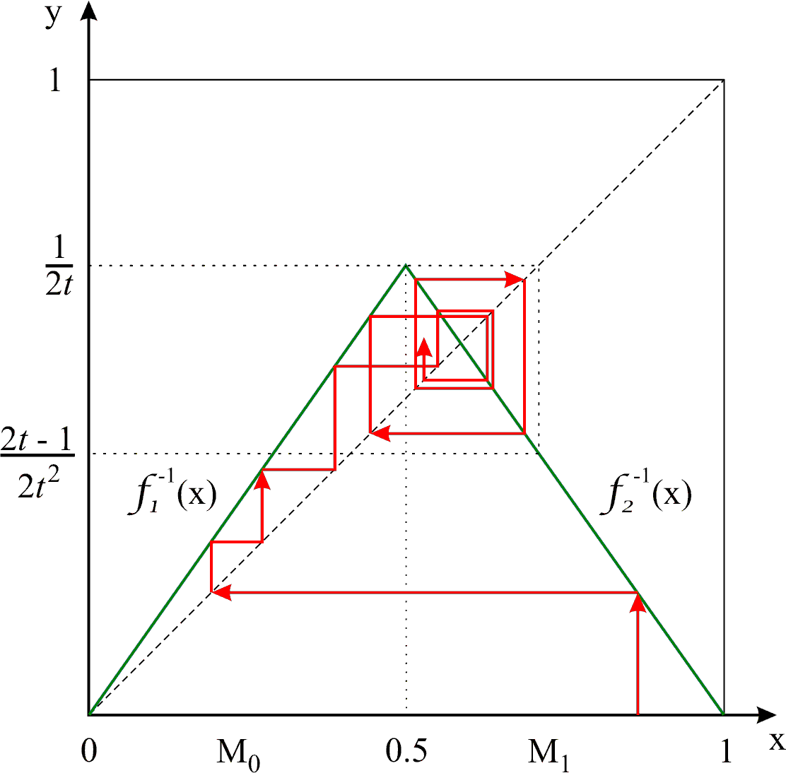
where $t\in[{\frac{1}{2},1)}$ is a parameter. The attractor of $A=[0,1].$ Let $M_{1}=[0,\frac{1}{2}],\ M_{2}=(\frac{1}{2},1]$ . Then the masked transformation

T(x)=\begin{cases}\frac{x}{t},&x\in M_{1},\\ \frac{1-x}{t},&x\in M_{2}\end{cases}

is continuous. This is the well-known one-parameter tent map dynamical system, see for example [12, Exercise 2.4.1, p.78]. We note that, for any $x\in(0,1)$ there exist a positive integer $n$ such that $T^{k}(x)\in\left[\frac{2t-1}{2t^{2}},\frac{1}{2t}\right]$ for all $k\geq n$ (see Fig. 2). As a consequence, if $\Lambda$ denotes the set of masked addresses of points in $\left[\frac{2t-1}{2t^{2}},\frac{1}{2t}\right]$ then the masked address space for $\mathcal{F}$ is

\underset{\text{n times}}{\{\underbrace{111...1}}\sigma|\sigma\in\Lambda,n=0,1,2,...\}\cup\underset{\text{n times}}{\{2\underbrace{111...1}}\sigma|\sigma\in\Lambda,n=0,1,2,...\}\text{.}

Theorem 18 concerns the relationship between masked address spaces corresponding to distinct masks. It has an application to packing multiple images into a single image, as illustrated in Example 25.

Theorem 18.

Let $\mathcal{F}$ be a point-fibred iterated function system with attractor $A$ . Let $T:A\rightarrow A$ be a masked dynamical system for $\mathcal{F}$ corresponding to mask $\mathcal{M}$ . Let $\mu$ be a measure on $A$ . Let $\mathcal{M}^{\prime}$ be a mask for $\mathcal{F}$ such that

\mu\left\{x\in A:\left\{T^{k}(x)\right\}_{k=0}^{\infty}\bigcap\left(\bigcup_{i\in I}\left(M_{i}\triangle M_{i}^{\prime}\right)\right)=\emptyset\right\}=0.

Let $\tau_{\mathcal{M}}$ and $\tau_{\mathcal{M}^{\prime}}$ be the masked sections of $\pi$ corresponding to $\mathcal{M}$ and $\mathcal{M}^{\prime}$ . Then $\tau_{\mathcal{M}}(x)\neq\tau_{\mathcal{M}^{\prime}}(x)$ for $\mu-$ almost all $x\in A$ .

Proof.

If $\tau_{\mathcal{M}}(x)=\tau_{\mathcal{M}^{\prime}}(x)$ it follows that $T^{k}(x)=T_{\mathcal{M}^{\prime}}^{k}(x)$ for all $k$ , where $T_{\mathcal{M}^{\prime}}:A\rightarrow A$ is the masked dynamical system corresponding to $\mathcal{M}^{\prime}$ . Then $T_{\mathcal{M}^{\prime}}^{k}(x)\notin\cup_{i\in I}\left(M_{i}\triangle M_{i}^{\prime}\right)$ for all $k$ . But this is impossible for $\mu-$ almost all $x\in A$ . ∎

4.2 (b) The fractal tops method

”Fractal tops” is the name we use to refer to the mathematics of tops functions, tops code spaces, tops dynamical systems, and associated fractal transformations; see for example [6, 7]. Here we show that, in the case where $\mathcal{F}$ is injective, fractal tops arise as a special case of masked iterated function systems. Specifically, a tops code space is a special case of masked address space, a tops function is a special case of a section of $\pi,$ and a tops dynamical system is a special case of a masked dynamical system. The computations associated with fractal tops tend to be less complicated than those for masked systems.

Define a dictionary ordering (see for example [17, p.26]) on $I^{\infty}$ as follows: if $\sigma,\omega\in I^{\infty}$ , $\sigma\neq\omega,$ then

\sigma<\omega\text{ iff }\sigma_{k}>\omega_{k},

where $k$ is the least index for which $\sigma_{k}\neq\omega_{k}$ , for all $\sigma,\omega\in I^{\infty}$ . With this ordering, every subset of $I^{\infty}$ possesses a greatest lower bound and a least upper bound. Since $\pi:I^{\infty}\rightarrow A\subset X$ is continuous and $I^{\infty}$ is compact, $\pi^{-1}(x)=\{\sigma\in I^{\infty}:\pi(\sigma)=x\}$ possesses a unique largest element, $\max\pi^{-1}(x)$ , for each $x\in A$ . This allows us to define an address space $\Omega\subset I^{\infty}$ for $\mathcal{F}$ by

\Omega=\{\max\pi^{-1}(x)|x\in A\}\text{.}

The corresponding section of $\pi$ is

\tau:A\rightarrow\Omega,\text{ }x\mapsto\max\pi^{-1}(x)\text{.}

If $\mathcal{F}$ is injective then the tops dynamical system is a masked dynamical system, corresponding to the mask defined by

M_{i}=f_{i}(A)\backslash\bigcup_{j=1}^{i-1}f_{j}(A),\ i\in I.

The fact that $\tau\left(x\right)$ can be computed from the set $\pi^{-1}(x)$ without reference to other points on the orbit of $x$ simplifies the computation of $\tau\left(x\right)$ in applications, see for example [5, 6]. Note that we can use the orbits of a tops dynamical system to calculate the top address of any point $x\in A$ according to $\tau(x)=\sigma_{1}\sigma_{2}...$ where

\sigma_{k}=\min\{n\in\{1,2,...,N\}:T^{\circ(k-1)}(x)\in f_{n}(A)\}.

5 Applications and examples

5.1 Application to image synthesis

Here we generalize the technique of color-stealing, introduced in [2] and implemented for example in [18, p.65-66].

Define a picture to be a function of the form

\mathfrak{P}:D\subset\mathbb{R}^{2}\rightarrow\mathfrak{C}

where $\mathfrak{C}$ is a color space. The set $D$ is the domain of the picture. We are concerned with situations where $D$ is a subset of an attractor of an iterated function system.

Let $\mathcal{F}$ be an injective iterated function system with attractor $A\subset\mathbb{R}^{2}$ . Let $\mathcal{F}^{\prime}$ be an iterated function system with attractor $A^{\prime}\subset\mathbb{R}^{2}$ and the same code space $I^{\infty}$ as for $\mathcal{F}$ . Let $\mathcal{M}$ be a mask for $\mathcal{F}$ and let $\tau_{\mathcal{M}}$ be the corresponding section of $\pi^{-1}.$ Let $\pi^{\prime}$ be the coding map for $\mathcal{F}^{\prime}$ . Then we can define a mapping $\Phi$ from the space of pictures on $A^{\prime}$ into the space of pictures on $A$ according to

\Phi_{\mathcal{M}}(\mathfrak{P}^{\prime})=\mathfrak{P}^{\prime}\circ\pi^{\prime}\circ\tau_{\mathcal{M}}.

We refer to this procedure as color-stealing because colors from the picture $\mathfrak{P}^{\prime}$ are mapped onto the attractor $A$ to define the new picture $\mathfrak{P}=\Phi_{\mathcal{M}}(\mathfrak{P}^{\prime})$ .

It follows from Theorem 16 (i) that the transformation $\pi^{\prime}\circ\tau_{\mathcal{M}}$ is continuous at all points $x\in A$ whose orbits lie in $A\backslash$ $\cup_{k=0}^{\infty}\mathcal{F}^{k}(\cup_{i\in I}\partial M_{i}),$ where $\partial M_{i}$ denotes the boundary of $M_{i}$ . In some cases, such as those in Example 19, $\cup_{k=0}^{\infty}\mathcal{F}^{k}(\cup_{i\in I}\partial M_{i})$ is a set of Lebesgue measure zero, so the transformation is continuous almost everywhere. This explains patches of similar colors tends to exist in pictures that are obtained by color-stealing from real world photos, where patches of similar colors occur for physical reasons.

Example 19.

Figure 3 illustrates color-stealing using (i) fractal tops (left), and (ii) a masked iterated function system (right) that is not a tops system. The picture $\mathfrak{B}^{\prime}$ from which colors are stolen is Lena embedded in a black surround, shown in the middle panel. In (i) $\mathcal{F}^{\prime}$ is an affine iterated function system whose attractor $A^{\prime}$ is a filled square, the domain of $\mathfrak{B}^{\prime}$ , such that $\{f_{i}^{\prime}(A^{\prime})\}_{i=1}^{4}$ is a set of tiles that tile $A^{\prime}$ by rectangles. In (i) $\mathcal{F}$ is the projective iterated function system $(\mathbb{RP}^{2};f_{1},f_{2},f_{3},f_{4})$ , where

f_{n}(x,y)=(\frac{a_{n}x+b_{n}y+c_{n}}{g_{n}x+h_{n}y+j_{n}},\frac{d_{n}x+e_{n}y+k_{n}}{g_{n}x+h_{n}y+j_{n}})\text{ for }n=1,2,3,4\text{;}

119.050.721.86−0.1516.9−0.285.632.0120.020.24.47.5−0.3−4.4−10.40.28.815.4396.535.25.8−131.4−6.519.1134.830.77.54−32.55.81−2.9122.9−0.1−19.9−128.1−24.3−5.8.\begin{tabular}[c]{|c|c|c|c|c|c|c|c|c|c|}\hline\cr$n$&$a_{n}$&$b_{n}$&$c_{n}$&$d_{n}$&$e_{n}$&$k_{n}$&$g_{n}$&$h_{n}$&$j_{n}$\\ \hline\cr$1$&$19.05$&$0.72$&$1.86$&$-0.15$&$16.9$&$-0.28$&$5.63$&$2.01$&$20.0$\\ $2$&$0.2$&$4.4$&$7.5$&$-0.3$&$-4.4$&$-10.4$&$0.2$&$8.8$&$15.4$\\ $3$&$96.5$&$35.2$&$5.8$&$-131.4$&$-6.5$&$19.1$&$134.8$&$30.7$&$7.5$\\ $4$&$-32.5$&$5.81$&$-2.9$&$122.9$&$-0.1$&$-19.9$&$-128.1$&$-24.3$&$-5.8$\\ \hline\cr\end{tabular}.

	$\begin{tabular}[c]{\|c\|c\|c\|c\|c\|c\|c\|c\|c\|c\|}\hline\cr$n$&$a_{n}$&$b_{n}$&$c_{n}$&$d_{n}$&$e_{n}$&$k_{n}$&$g_{n}$&$h_{n}$&$j_{n}$\\ \hline\cr$1$&$19.05$&$0.72$&$1.86$&$-0.15$&$16.9$&$-0.28$&$5.63$&$2.01$&$20.0$\\ $2$&$0.2$&$4.4$&$7.5$&$-0.3$&$-4.4$&$-10.4$&$0.2$&$8.8$&$15.4$\\ $3$&$96.5$&$35.2$&$5.8$&$-131.4$&$-6.5$&$19.1$&$134.8$&$30.7$&$7.5$\\ $4$&$-32.5$&$5.81$&$-2.9$&$122.9$&$-0.1$&$-19.9$&$-128.1$&$-24.3$&$-5.8$\\ \hline\cr\end{tabular}.$	$n$	$a_{n}$	$b_{n}$	$c_{n}$	$d_{n}$	$e_{n}$	$k_{n}$	$g_{n}$	$h_{n}$	$j_{n}$

and $\mathcal{F}^{\prime}$ is an affine IFS whose attractor is a filled square; see also [5, p.2]. In (ii) the iterated function system $\mathcal{F}$ and mask $\mathcal{M}$ are the same as in Example 23, while $\mathcal{F}^{\prime}$ is a perturbed version of $\mathcal{G}$ in Example 23.

5.2 Fractal homeomorphisms for image beautification, roughening, and special effects

Under the conditions of Theorem 10 (ii) the fractal transformation $T_{\mathcal{FG}}$ is a homeomorphism. Such homeomorphisms can be applied to pictures to yield new pictures that have the same topological properties as the original. For example the connectivity properties of the set defined by a particular color will be preserved, as will be the property that certain colors lie in an arbitrary neighborhood of a point. But geometrical properties, such as Hausdorff dimension and collinearity, may not be preserved and, indeed, may be significantly changed.

Techniques for constructing and computing fractal homeomorphisms using fractal tops, with projective, affine, and bilinear IFSs, have been discussed in [2, 5, 6, 7, 18]. Families of fractal homeomorphisms, built from such transformations in $\mathbb{R}^{2}$ , may be established by using code space arguments. Typically, the attractors of the iterated function systems in question are non-overlapping, which simplifies the proofs: in some situations one only needs to show that the equivalence classes of addresses agree on certain straight line segments. The resulting families of transformations are described by a finite sets of real parameters. These parameters may be adjusted to achieve desired effects such as increased roughness, or continuous (but non-differentiable) transformation from a meaningless picture into a meaningful one. Both of these effects are illustrated in Example 20.

Example 20.

Figure 5 illustrates three fractal homeomorphisms of the unit square applied to Lena. All the iterated function systems involved are constructed using bilinear functions defined as follows. Let $\square=[0,1]^{2}\subset\mathbb{R}^{2}$ denote the unit square, with vertices $A=(0,0),B=(1,0),C=(1,1),D=(0,1).$ Let $P,Q,R,S$ denote, in cyclic order, the successive vertices of a possibly degenerate quadrilateral. We uniquely define a bilinear function $\mathcal{B}:\mathcal{R}\rightarrow\mathcal{R}$ such that $\mathcal{B}(ABCD)=PQRS$ by

\mathcal{B}(x,y)=P+x(Q-P)+y(S-P)+xy(R+P-Q-S).

This transformation acts affinely on any straight line that is parallel to either the $x$ -axis or the $y$ -axis. For example, if $\mathcal{B}|_{AB}:AB\rightarrow PQ$ is the restriction to $AB$ of $\mathcal{B}$ and if $\mathcal{Q}:\mathbb{R}^{2}\rightarrow\mathbb{R}^{2}$ is the affine function defined by $\mathcal{Q}(x,y)=P+x(Q-P)+y(S-P),$ then $\mathcal{Q}|_{AB}=\mathcal{B}|_{AB}$ . Sufficient conditions for a bilinear iterated function system to be point-fibred are given in [7]. Each homeomorphism in Figure 5 is generated using a pair of iterated function systems of the form in Figure 4; each such pair has the same address structure.

The following theorem provides practical sufficient conditions for a bilinear IFS to be hyperbolic.

It is more difficult to establish conditions under which pairs of masked overlapping iterated function systems, built from geometrical functions such as affines on $\mathbb{R}^{2},$ yield homeomorphisms. In order to establish that a pair of masked iterated function systems provides a fractal transformation that is a homeomorphism, it is necessary to establish that the two masked address spaces agree. Interesting non-trivial cases involve overlapping iterated function systems, and cannot be reformulated as fractal tops. A beautiful family of such examples is provided by Theorem 21.

Theorem 21.

Let $\mathcal{F}=([0,1],f_{1}(x)=ax,f_{2}(x)=by+(1-b)),$ where $a\geq b>0,$ and $a+b\geq 1,$ have mask $M^{(p)}=\{M_{1},M_{2}\}$ where $M_{1}=[0,p]$ , $M_{2}=(p,1],$ and $p\in[1-b,a]$ . Let $\mathcal{G}=([0,1],g_{1}(x)=bx,g_{2}(x)=ay+(1-a))$ have mask $M^{(1-p)}$ . Then there exists $p^{\ast}\in[1-b,a]$ such that the corresponding fractal transformation $T_{\mathcal{FG}}:[0,1]\rightarrow[0,1]$ is a homeomorphism when $p=p^{\ast}.$ The inverse of this homeomorphism is $T_{\mathcal{GF}}:[0,1]\rightarrow[0,1]$ defined by associating the mask $M^{(1-p^{\ast})}$ with $\mathcal{G}$ .

Proof.

This is an outline. Let $\square=[0,1]^{2}\subset\mathbb{R}^{2}$ . Define affine transformations by

	$\displaystyle W_{-}$	$\displaystyle:\mathbb{R}^{2}\rightarrow\mathbb{R}^{2},(x,y)\mapsto(ax,by),$
	$\displaystyle W_{+}$	$\displaystyle:\mathbb{R}^{2}\rightarrow\mathbb{R}^{2},(x,y)\mapsto(bx+1-b,ay+1-y).$

Let $S_{-}=\{(x,y)\in\mathbb{R}^{2}:x+y\leq 1\}$ and $S_{+}=\mathbb{R}^{2}\backslash S_{-}$ . We consider the dynamical system

Q:\mathbb{R}^{2}\rightarrow\mathbb{R}^{2},(x,y)\mapsto\left\{\begin{array}[c]{c}W_{-}^{-1}(x,y)\text{ if }(x,y)\in S_{-},\\ W_{+}^{-1}(x,y)\text{ if }(x,y)\in S_{+}.\end{array}\right.

This possesses a ”repeller”, a compact set $\mathcal{R}\subset\square,$ such that

\mathcal{R}=Q(\mathcal{R})\text{.}

In order to define $\mathcal{R}$ , we define

W:K\left(\square\right)\rightarrow K\left(\square\right),C\mapsto(S_{-}\cap W_{-}(C))\cup(\overline{S_{+}}\cap W_{+}(C)),

and

\mathcal{R}=\lim_{k\rightarrow\infty}W^{k}(\square).

$\mathcal{R}$ is well-defined because it is the intersection of a decreasing sequence of nonempty compact sets. (It is quite easy to see that $\mathcal{R}$ is the graph of a monotone function from $[0,1]$ onto $[0,1].$ ) Using symmetry about the line $x+y=1$ and the contractivity of $W_{-}$ and $W_{+}$ in both the $x$ and $y$ directions it can be proved that $\mathcal{R}$ has the following properties.

(i) $Q(\mathcal{R})=\mathcal{R};$

(ii) $\mathcal{R}$ is symmetrical about the line $x+y=1;$

(iii) $P_{-}(\mathcal{R})=P_{+}(\mathcal{R})=[0,1],$ where $P_{-}:\mathbb{R}^{2}\rightarrow\mathbb{R}$ denotes the projection in the $x$ direction and $P_{+}:\mathbb{R}^{2}\rightarrow\mathbb{R}$ denotes projection in the $y$ direction;

(iv) there is a continuous, monotone strictly increasing function $\Phi:[0,1]\rightarrow[0,1],$ such that $\Phi(0)=0$ , $\Phi(1)=1$ , $\Phi(1-\Phi(x))=1-x$ for all $x\in[0,1],$ and $\mathcal{R}=\{(x,\Phi(x)):x\in[0,1]\}$ ;

(v) there is a unique $p^{\ast}\in[1-b,a]$ such that $\Phi(p^{\ast})=1-p^{\ast};$

(vi) there is a continuous, monotone strictly increasing function, $\Psi:[0,1]\rightarrow[0,1],$ such that $\Psi(0)=0$ , $\Psi(1)=1$ , $\Psi(1-\Psi(y))=1$ for all $y\in[0,1]$ , and $\mathcal{R}=\{(y,1-\Psi(1-y)):y\in[0,1]\}$ ;

(vii) $\Psi(1-p^{\ast})=p^{\ast};$

(viii) $\Psi(y)=\Phi^{-1}(y)$ for all $y\in[0,1]$ ;

(ix) if $p=p^{\ast}$ , then the masked dynamical system $T_{\mathcal{F}}:[0,1]\rightarrow[0,1]$ obeys

T_{\mathcal{F}}(x)=P_{-}(Q(x,\Phi(x)))\text{ for all }x\in[0,1];

(x) if $p=p^{\ast}$ , then the masked dynamical system $T_{\mathcal{G}}:[0,1]\rightarrow[0,1]$ obeys

T_{\mathcal{G}}(y)=P_{+}(Q(\Psi(y),y))\text{ for all }y\in[0,1].

These statements imply the theorem. ∎

Remark 22.

Clearly essentially the same result and proof applies for any analogous pair of overlapping strictly increasing functions on $[0,1]$ .

Figure 6 illustrates the ”repeller”. It is a subset of the attractor of the iterated function system $(\square;(ax,by),(bx+1-b,ay+1-a)),$ and may be used to compute $p^{\ast}$ as illustrated in Figure 7.

An example of a fractal transformation, arising from a masked pair of overlapping affine iterated function systems, is given in Example 23. The resulting homeomorphism with $a=\frac{2}{3}$ and $b=\frac{1}{2}$ yields a picture of Lena with extra large eyes, Figure 1.

Example 23.

Let $\mathcal{H}_{p,q}:=(X;h_{1},h_{2},h_{3},h_{4})$ be the family of affine iterated function systems defined by $X\mathbb{=\{}(x,y)\in\mathbb{R}^{2}|0\leq x,y\leq 1\},$ $r,s\in(0,1),$

	$\displaystyle h_{1}(x,y)$	$\displaystyle=(rx,ry),h_{2}(x,y)=(sx+1-s,ry),$
	$\displaystyle h_{3}(x,y)$	$\displaystyle=(sx+1-s,sy+1-s),h_{4}(x,y)=(rx,sy+1-s).$

Let $\mathcal{F}=\mathcal{H}_{\frac{2}{3},\frac{1}{2}}$ and, for $p\in[\frac{1}{2},\frac{2}{3}],$ let $M_{p}$ be the mask $\{M_{1},M_{2},M_{3},M_{4}\}$ where

	$\displaystyle M_{1}$	$\displaystyle=\{(x,y)\in X:x\leq p,y\leq p\},M_{2}=\{(x,y)\in X:x>p,y\leq p\},$
	$\displaystyle M_{3}$	$\displaystyle=\{(x,y)\in X:x>p,y>p\},M_{4}=\{(x,y)\in X:x\leq p,y>p\}.$

Let $\mathcal{G}=\mathcal{H}_{\frac{1}{2},\frac{2}{3}}.$ Then, by Theorem 21, there is a value of $p=$ $p^{\ast}\in(\frac{1}{2},\frac{2}{3}),$ such that the condition in Theorem 10 (ii) holds, and if $p=p^{\ast}$ then $T_{\mathcal{FG}}:X\rightarrow X$ then is a homeomorphism. The value of $p^{\ast}$ is

p^{\ast}=\max\{p\in(\frac{1}{2},\frac{2}{3}):(p,1-p)\in A^{\ast}\}

where $A^{\ast}\subset X$ is the attractor of $\mathcal{H}:=(X;(\frac{2}{3}x,\frac{1}{2}y),(\frac{1}{2}x+\frac{1}{2},\frac{2}{3}y+\frac{1}{3}))$ illustrated in Figure 7. Experimentally we find $p^{\ast}\doteq 0.618$ which is used to compute Figure 1. The original Lena was overlayed on a black background, as in Figure 3. The transformed picture also had a black background that has been omitted here.

5.3 Application to image filtering

Here we restrict attention to iterated function systems defined on $X=[0,1]^{2}\subset$ $\mathbb{R}^{2}$ . We are concerned with fractal transformations from $[0,1]^{2}$ to itself, associated with a pair of iterated function systems of the form

\mathcal{F}=([0,1]^{2},f_{1},f_{2},...,f_{N})\text{, }\mathcal{G}=([0,1]^{2},g_{1},g_{2},...,g_{N}).

We suppose that $A_{\mathcal{F}}=A_{\mathcal{G}}=[0,1]^{2}$ . In applications to digital imaging, $[0,1]^{2}$ is discretized. Here we refer to the the locations of pixels as discretized coordinates. We suppose that discretized versions of $A_{\mathcal{F}}$ and $A_{\mathcal{G}}$ have resolutions $r_{\mathcal{F}}$ and $r_{\mathcal{G}}$ respectively.

Let $P_{\mathcal{F}}:A_{\mathcal{F}}\rightarrow A_{\mathcal{F}}$ be a projection operator, namely a function with the property $P_{\mathcal{F}}\circ P_{\mathcal{F}}(x)=P_{\mathcal{F}}(x)$ for all $x\in A_{\mathcal{F}}$ . For example,

P_{\mathcal{F}}(x)=x\text{ discretized to resolution }r_{\mathcal{F}},\text{ for all }x\in[0,1]^{2}\text{.}

If $T_{\mathcal{FG}}:A_{\mathcal{F}}\rightarrow A_{\mathcal{G}}$ is a homeomorphism between the non-discretized spaces then

P_{\mathcal{G}}:=T_{\mathcal{FG}}\circ P_{\mathcal{F}}\circ T_{\mathcal{GF}}:A_{\mathcal{G}}\rightarrow A_{\mathcal{G}}

is also a projection operator because $T_{\mathcal{FG}}\circ T_{\mathcal{GF}}=i_{\mathcal{G}},$ the identity on $A_{\mathcal{G}},$ whence $P_{\mathcal{G}}\circ P_{\mathcal{G}}=T_{\mathcal{FG}}\circ P_{\mathcal{F}}\circ T_{\mathcal{GF}}\circ T_{\mathcal{FG}}\circ P_{\mathcal{F}}\circ T_{\mathcal{GF}}=T_{\mathcal{FG}}\circ P_{\mathcal{F}}\circ i_{\mathcal{F}}\circ P_{\mathcal{F}}\circ T_{\mathcal{GF}}=i_{\mathcal{G}}$ .

A trivial but instructive example is provided by choosing $\mathcal{F}$ and $\mathcal{G}$ to be the same, with $N=4$ and

	$\displaystyle f_{1}(x,y)$	$\displaystyle=(0.5x,0.5y),f_{2}(x,y)=(0.5x+0.5,0.5y),$
	$\displaystyle f_{3}(x,y)$	$\displaystyle=(0.5x+0.5,0.5y+0.5),f_{4}(x,y)=(0.5x,0.5y+0.5).$

If $r_{\mathcal{F}}=r_{\mathcal{G}}/2$ then $P_{\mathcal{G}}$ is the filter that corresponds to downsampling followed by doubling the width and height of each pixel.

Example 24.

Let $X\mathbb{=\{}(x,y)\in\mathbb{R}^{2}|0\leq x,y\leq 1\},$ $p\in(0,1)$ , $q=1-p,$ and

	$\displaystyle h_{1}(x,y)$	$\displaystyle=(px,py),h_{2}(x,y)=(qx+p,py),$
	$\displaystyle h_{3}(x,y)$	$\displaystyle=(qx+p,qy+p),h_{4}(x,y)=(px,qy+p).$

The family of IFSs $\mathcal{H}_{p}:=(X;h_{1},h_{2},h_{3},h_{4})$ has attractor $X$ and address structure that is independent of $p\in(0,1).$ If we set $\mathcal{F}=\mathcal{H}_{0.5}$ and $\mathcal{G}=\mathcal{H}_{0.6}$ then $T_{\mathcal{FG}}:X\mathbb{\rightarrow}X$ is a homeomorphism. The result of applying the fractal homeomorphism $T_{\mathcal{FG}}$ to a digital ( $512\times 512$ ) picture of Lena (left) is illustrated in the middle panel of Figure 8. In effect the middle image is obtained by composing a projection $P_{\mathcal{F}}$ , onto a $512\times 512$ pixel grid, with $T_{\mathcal{FG}}$ . The image on the right is the result of applying $T_{\mathcal{GF}}$ to the middle image. that is, the right-hand image is the result of applying the projection operator, that we may refer to as a ”fractal filter”, $T_{\mathcal{GF}}\circ P_{\mathcal{F}}\circ$ $T_{\mathcal{FG}}$ to the original Lena.

5.4 Application to packing multiple images into a single image

Suppose we have a collection of masks $\{\mathcal{M}_{j}\}$ on $A$ such that the conditions of Lemma 18 are holds true for any pair of masks. Let the second iterated function system $\mathcal{F}^{\prime}$ be such that almost all points of the attractor $A^{\prime}$ have a unique address. Thus by Lemma 18

\pi^{\prime}\circ\tau_{\mathcal{M}_{j}}(x)\neq\pi^{\prime}\circ\tau_{\mathcal{M}_{k}}(x)

for almost all $x\in A$ and $j\neq k$ . Therefore we can consider the collection of pictures $\Phi_{\mathcal{M}_{j}}(\mathfrak{B}^{\prime})$ as an almost disjoint fractal decomposition of the picture $\mathfrak{B}^{\prime}$ .

This leads us to the following trick. By means of fractal transformations we map different pictures to different almost disjoint components of $\mathfrak{B}^{\prime}$ . By inverting the transformations we retrieve (approximations to) the original pictures, as illustrated in the following example.

Example 25.

See Figure 9. Let

\mathcal{F}=(\square,f_{1}(x,y)=(y,0.6(1-x)),f_{2}(x,y)=(y,0.4+0.6x))

and

\mathcal{G}=(\square,f_{1}(x,y)=(y,0.5(1-x)),f_{2}(x,y)=(y,0.5+0.5x)).

We define a family of masks for $\mathcal{F}$ by

\mathcal{M}_{p}=\{M_{1}=\{(x,y)\in\square:x\leq p\},M_{2}=\{(x,y)\in\square:x>p\}\},p\in[0.4,0.6].

$\square$ is the attractor of both systems. We denote the corresponding masked fractal transformation $T_{\mathcal{FG}}:\square\rightarrow\square$ by $T_{\mathcal{FG}}^{(p)}:\square\rightarrow\square,$ for $p\in[0.4,0.6]$ . Then $T_{\mathcal{FG}}^{(p)}$ is injective and invertible on its range, $T_{\mathcal{FG}}^{(p)}(\square)$ . Moreover, from Theorem 18 it follows that $\lambda(T_{\mathcal{FG}}^{(p)}(\square)\cap T_{\mathcal{FG}}^{(q)}(\square))=0$ for all $p\neq q$ , where $\lambda$ is Lebesgue measure. Let $\mathfrak{P}$ and $\mathfrak{Q}$ be two pictures, each supported on $\square$ . Then $T_{\mathcal{FG}}^{(p)}(\mathfrak{P)}=\mathfrak{P}\circ(T_{\mathcal{FG}}^{(p)})^{-1}$ is a picture supported on $T_{\mathcal{FG}}^{(p)}(\square)$ and $T_{\mathcal{FG}}^{(q)}(\mathfrak{Q)}=\mathfrak{Q}\circ(T_{\mathcal{FG}}^{(p)})^{-1}$ is a picture supported on $T_{\mathcal{FG}}^{(q)}(\square)$ . We choose $p=0.44,$ $q=0.56,$ $\mathfrak{P}=$ Lena and $\mathfrak{Q}=$ Inverted-Lena, where both pictures are $512\times 512$ . The digitized combined picture $\mathfrak{R}:=T_{\mathcal{FG}}^{(p)}(\mathfrak{P)}\cup T_{\mathcal{FG}}^{(q)}(\mathfrak{Q)}$ , also of resolution $512\times 512$ , is shown in the middle panel of Figure 9. Pixels which correspond to points in $T_{\mathcal{FG}}^{(p)}(\square)$ both $T_{\mathcal{FG}}^{(q)}(\square)$ are colored white. The left-hand panel in Figure 9 illustrates the picture $\mathfrak{R\circ}T_{\mathcal{FG}}^{(p)}$ and the right-hand panel shows $\mathfrak{R\circ}T_{\mathcal{FG}}^{(q)}$ . Hence we can ”store” the two pictureswe have that for each distinct choice of $p\in[0.4,0.6]$ the ranges of the $\mathcal{M}_{0.44}$ and $\mathcal{M}_{0.56}$ respectively.

5.5 Measure theory image packing

Here we describe a different method for encoding several images within a single image. The method strives to create a single image that is simultaneously ”homeomorphic”, under different fractal transformations, to several different given images. An example of such a single ”encoded” image is shown in the middle panel of Figure 10; two different fractal homeomorphisms applied to it (but in the digital realm) yield the images on the right and the left. The underlying idea is that different invariant measures, belonging to the same iterated function system, but associated with different probabilities, are mutually ”singular continuous”, and are concentrated on different sets, albeit they have the same support. The method uses the chaos game algorithm, both to encode and decode.

Consider for example the IFS $\mathcal{F}=([0,1];f_{1}(x)=0.5x,f_{2}(x)=0.5x+0.5)$ . If we associate probabilities $p_{1}=0.5$ and $p_{2}=0.5$ with $f_{1}$ and $f_{2}$ respectively, then the associated Markov operator has invariant probability measure $\mu$ equal to uniform Lebesgue measure supported on $[0,1]$ , concentrated on the set of points whose binary expansions contain equal proportions of zeros and ones. On the other hand, if we associate probabilities $\widetilde{p}_{1}=0.1$ and $\widetilde{p}_{2}=0.9,$ then the associated Markov operator has invariant probability measure $\widetilde{\mu}$ that is also supported on $[0,1]$ , but singular continuous and concentrated on the set of points whose binary expansions contain nine times as many ones as zeros. Hence, if the chaos game is applied to $\mathcal{F}$ using the first set of probabilities, the points of the resulting random orbit will tend to be disjoint from those obtained by of applying the chaos game using the second set of probabilities. The precise manner in which the orbits of the two systems concentrate is governed by convergence rates associated with the central limit theorem. The same idea can be applied to ”store” several images in a single image E: a stored image is retrieved by applying the appropriate fractal transformation to E.

We describe the method by means of an example.

Example 26.

We use three iterated function systems:

	$\displaystyle\mathcal{F}$	$\displaystyle=(\square,f_{1},f_{2},f_{3},f_{4}),\text{ }\mathcal{G}=(\square,g_{1},g_{2},g_{3},g_{4})\text{, }\mathcal{H}=(\square,h_{1},h_{2},h_{3},h_{4})\text{ where}$
	$\displaystyle f_{1}(x,y)$	$\displaystyle=(0.66x,0.34y),\text{ }f_{2}(x,y)=(0.34x+0.66,0.34y),$
	$\displaystyle f_{3}(x,y)$	$\displaystyle=(0.34x+0.66,0.66y+0.34),\text{ }f_{4}(x,y)=(0.66x,0.66y+0.34);$
	$\displaystyle g_{1}(x,y)$	$\displaystyle=(0.34x,0.66y),\text{ }g_{2}(x,y)=(0.66x+0.34,0.66y),$
	$\displaystyle g_{3}(x,y)$	$\displaystyle=(0.66x+0.34,0.34y+0.66),\text{ }g_{4}(x,y)=(0.34x,0.34y+0.66);$
	$\displaystyle h_{1}(x,y)$	$\displaystyle=(0.5x,0.5y),\text{ }h_{2}(x,y)=(0.5x+0.5,0.5y),$
	$\displaystyle h_{3}(x,y)$	$\displaystyle=(0.5x+0.5,0.5y+0.5),\text{ }h_{4}(x,y)=(0.5x,0.5y+0.5).$

Then $\mathcal{F}$ is associated with probabilies $P=\{p_{i}=area\left(f_{i}(\square\right)):$ $i=1,2,3,4\}$ Similarly the iterated function system $\mathcal{G}$ is associated with probabilities $\widetilde{P}=\{\widetilde{p}_{i}=area(g_{i}(\square)):i=1,2,3,4\}.$

The goal is to ”store” two standard digital color images, Pepper and Lena, each $512\times 512,$ in a single color image $E,$ also $512\times 512$ . The image $E$ is supported on $\square$ and associated with two probability measures, $\mu_{\mathcal{H}}$ and $\widetilde{\mu}_{\mathcal{H}},$ invariant under $\mathcal{H}$ with probabilities $P$ and $\widetilde{P}$ respectively.

(1) In order to ”encode” Pepper, we run a coupled chaos game algorithm with $\mathcal{F}$ associated with Pepper, supported on a copy of $\square,$ and $\mathcal{H}$ associated with $E,$ with (supposedly) i.i.d. probabilities $P$ ; that is, we compute a random sequence of points $\{(X_{k},Z_{k})\in\square\times\square:k=0,1,2,...K\}$ where $K=10^{6},$ where $X_{0}=(0,0)\in\square$ (associated with Pepper) and $Z_{0}=(0,0)\in\square$ (associated with $E$ ) and

X_{k}=f_{\sigma_{k}}(X_{k-1}),Z_{k}=h_{\sigma_{k}}(Z_{k-1})\text{ for }k=1,2,...,K,

where $\sigma_{k}=i$ with probability $p_{i}$ . At each step the pixel containing $Z_{k}$ in the (initially blank) image $E$ is plotted in the color of Pepper at the pixel containing $X_{k}$ . At the end of this process $E$ consists of an ”encoded” version of Pepper.

(2) In order to ”encode” Lena, we again run a coupled chaos game algorithm with $\mathcal{G}$ associated with Lena, supported on a copy of $\square,$ and $\mathcal{H}$ associated with $E$ (already ”painted” with an encoding of Pepper) with probabilities $\widetilde{P}$ ; that is, we compute a sequence of points $\{(Y_{k},\widetilde{Z}_{k})\in\square\times\square:k=0,1,2,...K\}$ where $K=500,000,$ where $Y_{0}=(0,0)\in\square$ (associated with Lena) and $Z_{0}=(0,0)\in\square$ (associated with $E$ ) and

Y_{k}=f_{\sigma_{k}}(Y_{k-1}),\widetilde{Z}_{k}=h_{\sigma_{k}}(\widetilde{Z}_{k-1})\text{ for }k=1,2,...,K,

where $\sigma_{k}=i$ with probability $\widetilde{p}_{i}$ . At each step the pixel containing $\widetilde{Z}_{k}$ in the image $E$ is plotted in the color of Lena at the pixel containing $Y_{k}$ . (The pixel is overwritten by the latest colour value.) We have used half as many iterations in the encoding of Lena as we did for Pepper, because a proportion of the points that correspond to Pepper are overwritten by points corresponding to Lena.

An image $E$ that is a realization of steps (1) and (2) is shown in the central panel of Figure 10. The image $E$ is approximately homeomorphic to both of the images Pepper and Lena, under the fractal transformations $T_{\mathcal{FH}}$ and $T_{\mathcal{GH}}$ respectively, that is

Pepper\doteq T_{\mathcal{FH}}(E)\text{ and }Lena\doteq T_{\mathcal{GH}}(E).

In practice, to obtain the decoded images, shown on the left and right hand sides of Figure 10, we use the chaos game algorithm again, as follows.

(3) In order to ”decode” Pepper, we run a coupled chaos game algorithm, with probabilities $P,$ with $\mathcal{F}$ associated with an image (initially blank), supported on a copy of $\square,$ and $\mathcal{H}$ associated with $E$ (now encoding both Pepper and Lena). That is, we compute a random sequence of points $\{(X_{k},Z_{k})\in\square\times\square:k=0,1,2,...K\}$ where $K=10^{6},$ where $X_{0}=(0,0)\in\square$ (associated with Pepper) and $Z_{0}=(0,0)\in\square$ (associated with $E$ ) and

X_{k}=f_{\sigma_{k}}(X_{k-1}),Z_{k}=h_{\sigma_{k}}(Z_{k-1})\text{ for }k=1,2,...,K,

where $\sigma_{k}=i$ with probability $p_{i}$ . At each step the pixel containing $X_{k}$ in the (initially blank) copy of $\square$ is plotted in the color of $E$ at the pixel containing $Z_{k}$ . The result of such a decoding, starting from the encoded $E$ illustrated in the middle panel, is shown in the left panel in Figure 10.

(4) In order to decode Lena, we run a coupled chaos game algorithm, with probabilities $\widetilde{P},$ with $\mathcal{G}$ associated with an image (initially blank but to become the decoded image), supported on a copy of $\square,$ and $\mathcal{H}$ associated with $E$ . That is, we compute a random orbit $\{(Y_{k},\widetilde{Z}_{k})\in\square\times\square:k=0,1,2,...K\}$ where $K=10^{6},$ where $Y_{0}=(0,0)\in\square$ (associated with Pepper) and $\widetilde{Z}_{0}=(0,0)\in\square$ (associated with $E$ ) and

Y_{k}=f_{\sigma_{k}}(X_{k-1}),\widetilde{Z}_{k}=h_{\sigma_{k}}(\widetilde{Z}_{k-1})\text{ for }k=1,2,...,K,

where $\sigma_{k}=i$ with probability $\widetilde{p}_{i}$ . At each step the pixel containing $Y_{k}$ in the (initially blank) copy of $\square$ is plotted in the color of $E$ at the pixel containing $\widetilde{Z}_{k}$ . The result of following this decoding algorithm, starting from the encoded $E$ in the middle panel, is shown in the left panel in Figure 10.

Acknowledgments

We thank Louisa Barnsley for help with the illustrations.

References

[1] Christoph Bandt, Karsten Keller, Self-similar sets 2. A simple approach to the topological structure of fractals, Math. Nachr. 154 (1991) 27-39.
[2] Michael F. Barnsley, Theory and applications of fractal tops, Fractals in Engineering: New Trends in Theory and Applications, Springer-Verlag, London, 2005. pp. 3-20.
[3] , Fractals Everywhere, Academic Press, Boston, 1988.
[4] , The life and survival of mathematical ideas, Notices Am. Math. Soc. 57 (2010) 10-22.
[5] , Superfractals, Cambridge University Press, Cambridge, 2006.
[6] , Transformations between self-referential sets, American Mathematical Monthly, 116 (2009) 291-304.
[7] , Transformations between fractals, Progress in Probability, 61 (2009) 227-250.
[8] Michael F. Barnsley and A. Vince, The Chaos Game on a General Iterated Function System, Ergodic Theory and Dynamical Systems, (2010) to appear.
[9] Michael F. Barnsley, Andrew Vince, David Wilson, Real projective iterated function systems, Preprint, 2010.
[10] John E. Hutchinson, Fractals and self-similarity, Indiana Univ. Math. J. 30 (1981) 713–747.
[11] Konstantin Igudesman, Top addresses for a certain family of iterated function systems on a segment, Russian Mathematics (Iz. VUZ), 53 (2009) 67-72.
[12] A. Katok and B. Hasselblatt, Introduction to the Modern Theory of Dynamical Systems. With a Supplementary Chapter by Katok and Leonardo Mendoza, Cambridge University Press, Cambridge, 1995.
[13] Bernd Kieninger, Iterated Function Systems on Compact Hausdorff Spaces, Shaker Verlag, Aachen, 2002.
[14] E. Klein, A.C. Thompson, Theory of Correspondences, Canadian Mathematical Society Series of Monographs and Advanced Texts. A Wiley-Interscience Publication, John Wiley & Sons, New York, 1984.
[15] Richard McGehee, Attractors for Closed Relations on Compact Hausdorff Spaces, Indiana University Mathematics Journal, 41 (1992) 1165-1209.
[16] B. Mendelson, Introduction to Topology (British edition), Blackie & Son, London, 1963.
[17] James R. Munkres, Topology, A First Course, Prentice-Hall, Inc., Englewood Cliffs, New Jersey, 1975.
[18] Slavomir Nikiel, Iterated Function Systems For Real Time Image Synthesis, Springer-Verlag London Limited, 2007.

How to transform and filter images using iterated function systems.

Abstract

keywords

AMS

1 Introduction

2 Point-fibred iterated function systems

Definition 1.

Theorem 2.

Proof.

Definition 3.

Theorem 4.

Proof.

Remark 5.

Definition 6.

3 Fractal transformations

Definition 7.

Theorem 8.

Proof.

Definition 9.

Theorem 10.

Proof.

Remark 11.

4 Construction of sections of π\pi

4.1 (a) The masked iterated function system method

Definition 12.

Definition 13.

Theorem 14.

Proof.

Definition 15.

Theorem 16.

Proof.

Example 17.

Theorem 18.

Proof.

4.2 (b) The fractal tops method

5 Applications and examples

5.1 Application to image synthesis

Example 19.

5.2 Fractal homeomorphisms for image beautification, roughening, and special effects

Example 20.

Theorem 21.

Proof.

Remark 22.

Example 23.

5.3 Application to image filtering

Example 24.

5.4 Application to packing multiple images into a single image

Example 25.

5.5 Measure theory image packing

Example 26.

Acknowledgments

References

4 Construction of sections of $\pi$