Discovery Potential of Selectron or Smuon as the Lightest Supersymmetric Particle at the LHC

Preprint: BONN-TH-2011-04, SCIPP 11/01

H. K. Dreiner Email: dreiner@th.physik.uni-bonn.de Affiliation: Bethe Center for Theoretical Physics and Physikalisches Institut, Universität Bonn, Bonn, Germany S. Grab Email: sgrab@scipp.ucsc.edu Affiliation: SCIPP, University of California Santa Cruz, Santa Cruz, CA 95064, USA T. Stefaniak Email: tim@th.physik.uni-bonn.de Affiliation: Bethe Center for Theoretical Physics and Physikalisches Institut, Universität Bonn, Bonn, Germany and II. Physikalisches Institut, Universität Göttingen, Göttingen, Germany

Abstract

We investigate the LHC discovery potential of $R$ -parity violating supersymmetric models with a right-handed selectron or smuon as the lightest supersymmetric particle (LSP). These LSPs arise naturally in $R$ -parity violating minimal supergravity models. We classify the hadron collider signatures and perform for the first time within these models a detailed signal over background analysis. We develop an inclusive three-lepton search and give prospects for a discovery at a center-of-mass energy of $\sqrt{s}=7$ TeV as well as $\sqrt{s}=14$ TeV. There are extensive parameter regions which the LHC can already test with $\sqrt{s}=7$ TeV and an integrated luminosity of 1 fb^-1. We also propose a method for the mass reconstruction of the supersymmetric particles within our models at $\sqrt{s}=14$ TeV.

I Introduction

Since 2010, the Large Hadron Collider (LHC) is collecting data at a center of mass energy of $\sqrt{s}=7$ TeV and first searches for physics beyond the Standard Model (SM) have been published [12, 1, 10, 2, 3, 4, 5, 6, 7, 8, 9, 11]. Even with only an integrated luminosity of 35 pb^-1, the LHC has already tested supersymmetric models [13, 14] beyond the Tevatron searches [11, 12]. Furthermore, it is expected that the LHC will collect 1 fb^-1 of data until the end of 2011.

One of the most promising LHC signatures for supersymmetry (SUSY) are multi-lepton final states [15, 16, 17]. On the one hand, electrons and muons are easy to identify in the detectors. On the other hand, the SM background for multi-lepton final states is low. In this publication, we focus on such signatures.

We consider the supersymmetric extension of the SM with minimal particle content (SSM) [13, 14]. Without further assumptions, the proton usually has a short lifetime in this model [18, 19, 20], in contradiction with experimental observations [21]. The proton decays, because renormalizable lepton and baryon number violating interactions are jointly present. One therefore must impose an additional discrete symmetry. The most common choice for this discrete symmetry is $R$ -parity, or equivalently at low-energy: proton-hexality ( $\text{P}_{6}$ ). Either suppresses all lepton- and baryon number violating interactions [22, 23, 24]. The SSM with $R$ -parity is usually denoted the minimal supersymmetric SM (MSSM).

We consider here a different discrete symmetry, baryon-triality ( $\text{B}_{3}$ ) [22, 23, 24, 25], which suppresses only the baryon number violating terms, but allows for lepton number violating interactions. The $\text{B}_{3}$ SSM has the advantage that neutrino masses are generated naturally [26, 27, 28, 29] without the need to introduce a new (see-saw) energy scale [30, 31, 32]. The lepton number violating interactions can be adjusted, such that the observed neutrino masses and mixing angles can be explained [33, 34]. Note that both P₆ and B₃ are discrete gauge anomaly free symmetries [22, 23, 35, 24].

In the $\text{B}_{3}$ SSM, the lightest supersymmetric particle (LSP) will decay via the lepton number violating interactions and is thus not bounded by cosmological observations to be the lightest neutralino, ${\tilde{\chi}}^{0}_{1}$ [37]. Unlike in the MSSM, the ${\tilde{\chi}}^{0}_{1}$ is not a valid dark matter (DM) candidate. However, several possible DM candidates are easily found in simple extensions of the $\text{B}_{3}$ SSM; for example, the axino [38, 39, 40, 41], the gravitino [42, 43] or the lightest $U$ -parity particle [44, 45].

We consider in this paper the $\text{B}_{3}$ SSM with a right-handed scalar electron (selectron, $\tilde{e}_{R}$ ) or scalar muon (smuon, $\tilde{\mu}_{R}$ ) as the LSP. These LSP candidates naturally arise in the $\text{B}_{3}$ minimal supergravity (mSUGRA) model [46], on which we focus in the following. Here, large lepton number violating interactions at the grand unification (GUT) scale drive the selectron or smuon mass towards small values at the electroweak scale via the renormalization group equations (RGEs) [47]. We describe this effect and the selectron and smuon LSP parameter space in the next section in more detail. Further LSP candidates within $\text{B}_{3}$ mSUGRA (beside the ${\tilde{\chi}}^{0}_{1}$ ) are the lightest stau, ${\tilde{\tau}}_{1}$ [46, 16, 48], and the sneutrino, $\tilde{\nu}_{e,\mu,\tau}$ [49, 46], depending on the dominant lepton number violating operator [47].

If SUSY exists, the pair production of strongly interacting SUSY particles (sparticles), like scalar quarks (squarks), is usually the main source for SUSY events at hadron colliders like the LHC [50]. Furthermore, squarks, $\tilde{q}$ , are much heavier than the ${\tilde{\chi}}^{0}_{1}$ in most supersymmetric models [51]. Assuming that we have a right-handed selectron or smuon, $\tilde{\ell}_{R}$ , as the LSP, a natural cascade process at the LHC is

\displaystyle\tilde{q}\tilde{q}\to qq{\tilde{\chi}}^{0}_{1}{\tilde{\chi}}^{0}_{1}\to qq\ell\ell\tilde{\ell}_{R}\tilde{\ell}_{R},

(1)

where the squarks decay into a quark, $q$ , and the ${\tilde{\chi}}^{0}_{1}$ . The ${\tilde{\chi}}^{0}_{1}$ decays into the $\tilde{\ell}_{R}$ LSP and an oppositely charged lepton, $\ell$ , of the same flavor.

The $\tilde{\ell}_{R}$ LSP can then decay via the lepton number violating interactions, for example

\displaystyle\tilde{\ell}_{R}\to\ell^{\prime}\nu,

(2)

i.e. into another charged lepton $\ell^{\prime}$ and a neutrino $\nu$ . As we argue in the following, this is the case for large regions of the $\text{B}_{3}$ SSM parameter space. We thus obtain from Eqs. (1) and (2) an event with four charged leptons in the final state. Taking into account that some leptons might not be well identified, we design in this paper an inclusive three-lepton search for $\tilde{\ell}_{R}$ –LSP scenarios. Although we concentrate on the $\text{B}_{3}$ mSUGRA model, our results apply also to more general models as long as Eqs. (1) and (2) hold. We will show that because of the high lepton multiplicity in B₃ models, the discovery reach at the LHC with $\sqrt{s}=7$ TeV exceeds searches in the $R$ -parity conserving case [52]. We also give prospects for a discovery at $\sqrt{s}=14$ TeV and propose a method for the reconstruction of sparticle masses within our model.

The phenomenology of slepton LSPs has mainly been investigated for the case of a stau LSP. See for example Refs. [46, 33, 53, 48, 56, 57, 58, 55, 59, 60, 61, 62, 54, 63, 16]. Recently, Ref. [16] proposed a tri-lepton search for stau LSP scenarios, which is similar to our analysis, although the stau in Ref. [16] decays via 4-body decays. LEP II has searched for slepton LSPs [64, 65]. No signals were found and lower mass limits around $90-100$ GeV were set. Refs. [54, 55] investigated the decay length of slepton LSPs assuming trilinear as well as bilinear $R$ -parity violating interactions. Finally, in Ref. [66], the signature of Eqs. (1) and (2) was pointed out. But in contrast to this work, no signal over background analysis was performed.

The remainder of this paper is organized as follows. In Sec. II we review the $\text{B}_{3}$ mSUGRA model and show how a $\tilde{\ell}_{R}$ LSP can arise. We present the ${\mathrm{B}_{\,\!3}}$ mSUGRA parameter regions with a $\tilde{\ell}_{R}$ LSP and propose a set of benchmark points for LHC searches. We then classify in Sec. III the $\tilde{\ell}_{R}$ LSP signatures at hadron colliders as a function of the dominant $R$ -parity violating interaction. Based on this, we develop in Sec. IV a set of cuts for an inclusive three-lepton search at the LHC and give prospects for a discovery at $\sqrt{s}=7$ TeV as well as at $\sqrt{s}=14$ TeV. In Sec. V we propose a method for the reconstruction of the supersymmetric particle masses. We conclude in Sec. VI.

Appendix A reviews the mass spectrum and branching ratios of our benchmark models and Appendix B shows the cutflow for our $\sqrt{s}=14$ TeV analysis. We give in Appendix C the relevant equations for the kinematic endpoints for the mass reconstruction of Sec. V and calculate in Appendix D some missing 3-body decays of sleptons.

II The Selectron and Smuon as the LSP in R-parity Violating mSUGRA

II.1 The ${\mathrm{B}_{\,\!3}}$ mSUGRA Model

In the ${\mathrm{B}_{\,\!3}}$ mSUGRA model the boundary conditions at the GUT scale ( $M_{\mathrm{GUT}}$ ) are described by the six parameters [46, 48]

\displaystyle M_{0},\,{M_{1/2}},\,A_{0},\,\tan\beta,\,\textrm{sgn}(\mu),\,\mathbf{\Lambda}.

(3)

Here, $M_{0}$ , ${M_{1/2}}$ and $A_{0}$ are the universal scalar mass, the universal gaugino mass and the universal trilinear scalar coupling, respectively. $\tan\beta$ denotes the ratio of the two Higgs vacuum expectation values (vevs), and $\textrm{sgn}(\mu)$ fixes the sign of the bilinear Higgs mixing parameter $\mu$ . Its magnitude is derived from radiative electroweak symmetry breaking [67]. $\mathbf{\Lambda}$ is described below.

In ${\mathrm{B}_{\,\!3}}$ mSUGRA, the superpotential is extended by the lepton number violating (LNV) terms [68],

\displaystyle W_{\mathrm{LNV}}=\frac{1}{2}{\bf\lambda}_{ijk}L_{i}L_{j}\bar{E}_{k}+{\bf\lambda}^{\prime}_{ijk}L_{i}Q_{j}\bar{D}_{k}+\kappa_{i}L_{i}H_{2},

(4)

which are absent in the MSSM. Here, $L_{i}$ and $Q_{i}$ denote the lepton and quark $SU(2)$ doublet superfields, respectively. $H_{2}$ is the Higgs $SU(2)$ doublet superfield which couples to up-type quarks, and $\bar{E}_{i}$ and $\bar{D}_{i}$ denote the lepton and down-type quark $SU(2)$ singlet superfields, respectively. $i,j,k\in\{1,2,3\}$ are generation indices. ${\bf\lambda}_{ijk}$ is anti-symmetric in the first two indices ( $i\leftrightarrow j$ ) and thus denotes nine, ${\bf\lambda}^{\prime}_{ijk}$ twenty-seven dimensionless couplings. The bilinear lepton number violating couplings $\kappa_{i}$ are three dimensionful parameters, which vanish in ${\mathrm{B}_{\,\!3}}$ mSUGRA at $M_{\mathrm{GUT}}$ due to a redefinition of the lepton and Higgs superfields [46]. However, they are generated at lower scales via RGE running with interesting phenomenological consequences for neutrino masses [34, 29].

In the ${\mathrm{B}_{\,\!3}}$ mSUGRA model, we assume that exactly one of the thirty-six dimensionless couplings in Eq. (4) is non-zero and positive at the GUT scale¹¹ 1 On the one hand, bounds on products of two different couplings are in general much stronger than on single couplings [69]. On the other hand, one observes also a large hierarchy between the Yukawa couplings within the SM.. The parameter $\mathbf{\Lambda}$ in Eq. (3) refers to this choice, i.e.

\displaystyle\mathbf{\Lambda}\in\{{\bf\lambda}_{ijk},\,{\bf\lambda}^{\prime}_{ijk}\},\qquad i,j,k=1,2,3.

(5)

Given one coupling at the GUT scale, other couplings that violate only the same lepton number are generated at the weak scale, $M_{Z}$ , by the RGEs [46, 53, 70, 71].

II.2 The Selectron and Smuon LSP

II.2.1 Renormalization Group Evolution of the $\tilde{\ell}_{R}$ Mass

In order to understand the dependence of the right-handed slepton ²² 2 We consider only the first two generations of sleptons, i.e. $\tilde{\ell}_{R}\in\{\tilde{e}_{R},\tilde{\mu}_{R}\}$ , because a stau LSP can also be obtained without (large) $R$ -parity violating interactions [46, 48]., $\tilde{\ell}_{R}$ , mass at $M_{Z}$ on the boundary conditions at $M_{\mathrm{GUT}}$ , we have to take a closer look at the relevant RGEs, which receive additional contributions from the LNV terms in Eq. (4). The dominant one-loop contributions to the running mass of the right-handed slepton of generation $k=1,2$ are [46]

		$\displaystyle 16\pi^{2}\frac{d(M_{\tilde{\ell}^{k}_{R}}^{2})}{dt}=-\frac{24}{5}g_{1}^{2}\|M_{1}\|^{2}+\frac{6}{5}g_{1}^{2}\mathcal{S}+2(\mathbf{h_{E^{k}}})_{ij}^{2}$
		$\displaystyle\;\;\;\;\;\;+4\lambda_{ijk}^{2}\left[(\mathbf{m_{\tilde{L}}}^{2})_{ii}+(\mathbf{m_{\tilde{L}}}^{2})_{jj}+(\mathbf{m_{\tilde{E}}}^{2})_{kk}\right]$		(6)

with

\displaystyle(\mathbf{h_{E^{k}}})_{ij}\equiv\lambda_{ijk}\times A_{0}\qquad\mbox{at}\quad M_{\mathrm{GUT}},

(7)

and

	$\displaystyle\mathcal{S}=$	$\displaystyle{~\rm Tr}[\mathbf{m_{\tilde{Q}}}^{2}-\mathbf{m_{\tilde{L}}}^{2}-2\mathbf{m_{\tilde{U}}}^{2}+\mathbf{m_{\tilde{D}}}^{2}+\mathbf{m_{\tilde{E}}}^{2}]$
		$\displaystyle+m_{H_{2}}^{2}-m_{H_{1}}^{2}.$		(8)

Here, $g_{1}$ ( $M_{1}$ ) is the $U$ (1) gauge coupling (gaugino mass) and $t=\ln Q$ with $Q$ the renormalization scale. $(\mathbf{h_{E^{k}}})_{ij}$ is the trilinear scalar soft breaking coupling corresponding to $\lambda_{ijk}$ . The bold-faced soft mass parameters in Eq. (6) and Eq. (8) are $3\times 3$ matrices in flavor space: $\mathbf{m_{\tilde{Q}}}$ and $\mathbf{m_{\tilde{L}}}$ for the left-handed doublet squarks and sleptons, $\mathbf{m_{\tilde{U}}}$ , $\mathbf{m_{\tilde{D}}}$ and $\mathbf{m_{\tilde{E}}}$ for the singlet up-squarks, down-squarks and sleptons, respectively. $m_{H_{1}}$ and $m_{H_{2}}$ are the scalar Higgs softbreaking masses.

The first two terms on the right-hand side in Eq. (6) are proportional to the gauge coupling squared, $g_{1}^{2}$ , and also present in $R$ -parity conserving models. The sum of these two terms is negative at any scale and thus leads to an increase of $M_{\tilde{\ell}^{k}_{R}}$ when running from $M_{\mathrm{GUT}}$ down to $M_{Z}$ . Here, the main contribution comes from the term proportional to the gaugino mass squared, $M_{1}^{2}$ , because $\mathcal{S}$ is identical to zero at $M_{\mathrm{GUT}}$ for universal scalar masses. Moreover, the coefficient of the $M_{1}^{2}$ term is larger than that of the $\mathcal{S}$ term.

The remaining contributions are proportional to $\lambda_{ijk}^{2}$ and $(\mathbf{h_{E^{k}}})^{2}_{ij}$ ; the latter implies also a proportionality to $\lambda_{ijk}^{2}$ at $M_{\mathrm{GUT}}$ , cf. Eq. (7). These terms are positive and will therefore reduce $M_{\tilde{\ell}^{k}_{R}}$ , when going from $M_{\mathrm{GUT}}$ down to $M_{Z}$ . They are new to the $\mathrm{B}_{3}$ mSUGRA model compared to $R$ -parity conserving mSUGRA. We can see from Eq. (6), that if the LNV coupling is roughly of the order of the gauge coupling $g_{1}$ , i.e. ${\bf\lambda}_{ijk}\gtrsim\mathcal{O}(10^{-2})$ , these terms contribute substantially. Then, the $\tilde{\ell}_{R}$ can be lighter than the lightest neutralino, ${\tilde{\chi}}^{0}_{1}$ , and lightest stau, $\tilde{\tau}_{1}$ , at $M_{Z}$ , leading to a $\tilde{\ell}_{R}$ LSP [47].

$L_{i}L_{j}\bar{E}_{k}$	LSP candidate	$2\sigma$ bound
${\bf\lambda}_{121}$ , ${\bf\lambda}_{131}$	$\tilde{e}_{R}$	$0.020\times(M_{\tilde{e}_{R}}/100\mbox{~GeV})$
${\bf\lambda}_{231}$	$\tilde{e}_{R}$	$0.033\times(M_{\tilde{e}_{R}}/100\mbox{~GeV})$
${\bf\lambda}_{132}$	$\tilde{\mu}_{R}$	$0.020\times(M_{\tilde{\mu}_{R}}/100\mbox{~GeV})$

Table 1: List of

L_{i}L_{j}\bar{E}_{k}

couplings (first column) needed to generate a

\tilde{e}_{R}

- or

\tilde{\mu}_{R}

-LSP (second column). The third column gives the most recent experimental bounds [

95\%

confidence level (C.L.)], taken from Ref. [72]. The bounds apply at

M_{\rm GUT}

. The bounds on

{\bf\lambda}_{212}

and

{\bf\lambda}_{232}

from the generation of too large neutrino masses are in general too strong to allow for a

\tilde{\mu}_{R}

-LSP [46], although exceptions might exist [29].

The respective $L_{i}L_{j}\bar{E}_{k}$ couplings $\mathbf{\Lambda}$ , which can lead to a $\tilde{e}_{R}$ or $\tilde{\mu}_{R}$ LSP, are given in Table 1 with their most recent experimental $2\sigma$ upper bounds at $M_{\rm GUT}$ [72]. Because of its RGE running, $\mathbf{\Lambda}$ at $M_{Z}$ is roughly 1.5 times larger than at $M_{\mathrm{GUT}}$ [71, 73].

Refer to caption — Figure 1: Masses of the $\tilde{e}_{R}$ , ${\tilde{\chi}}^{0}_{1}$ , $\tilde{\tau}_{1}$ , $\tilde{\tau}_{2}$ , ${\tilde{\nu}_{\tau}}$ , $\tilde{\mu}_{L}$ and ${\tilde{\nu}_{\mu}}$ at $M_{Z}$ as a function of $\lambda_{231}$ at $M_{\mathrm{GUT}}$ . The other mSUGRA parameters are $M_{0}=150\mbox{~GeV}$ , ${M_{1/2}}=500\mbox{~GeV}$ , $A_{0}=-1000\mbox{~GeV}$ , $\tan\beta=5$ and $\mu>0$ . The yellow region corresponds to the experimentally allowed $\tilde{e}_{R}$ LSP region. The gray patterned region is excluded by the upper bound on ${\bf\lambda}_{231}$ , cf. Table 1.

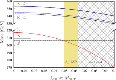
As an example, in Fig. 1, we demonstrate the impact of a non-vanishing coupling $\lambda_{231}$ at $M_{\rm GUT}$ on the running of the $\tilde{e}_{R}$ mass. Note that we can obtain a $\tilde{e}_{R}$ LSP ( $\tilde{\mu}_{R}$ LSP) with a non-zero coupling ${\bf\lambda}_{121}$ or ${\bf\lambda}_{131}$ ( ${\bf\lambda}_{132}$ ) at $M_{\mathrm{GUT}}$ in a completely analogous way. We employ SOFTSUSY3.0.13 [74, 75] for the evolution of the RGEs. We have chosen a fairly large absolute value of $A_{0}=-1000\mbox{~GeV}$ (see the discussion in Sec. II.2.2). The other mSUGRA parameters are $M_{0}=150\mbox{~GeV}$ , ${M_{1/2}}=500\mbox{~GeV}$ , $\tan\beta=5$ and $\mu>0$ . In the corresponding $R$ -parity conserving case ( ${\bf\lambda}_{231}|_{\rm GUT}=0$ ), the ${\tilde{\chi}}^{0}_{1}$ is the LSP and the $\tilde{\tau}_{1}$ is the next-to LSP (NLSP).

The $\tilde{e}_{R}$ mass decreases for increasing $\lambda_{231}$ , as described by Eq. (6). Furthermore, the masses of the (mainly) left-handed second and third generation sleptons, $\tilde{\mu}_{L}$ , $\tilde{\tau}_{2}$ , and sneutrinos, ${\tilde{\nu}_{\mu}}$ , ${\tilde{\nu}_{\tau}}$ , decrease³³ 3 However, these (negative) $R$ -parity violating contributions are always smaller than those to the right-handed slepton mass [46]. Thus, the left-handed sleptons and sneutrinos cannot become the LSP within ${\mathrm{B}_{\,\!3}}$ mSUGRA with ${\bf\lambda}_{ijk}|_{\rm GUT}\not=0$ [47]., since these fields couple directly via $\lambda_{231}$ . In contrast, the mass of the ${\tilde{\chi}}^{0}_{1}$ is not changed, since it does not couple to the ${\bf\lambda}_{231}$ operator at one loop level. Also the impact on the mass of the $\tilde{\tau}_{1}$ , which is mostly right-handed, is small. We therefore obtain in Fig. 1 at $\lambda_{231}|_{\mathrm{GUT}}\gtrsim 0.05$ a right-handed selectron as the LSP.

Because of the experimental upper bound on ${\bf\lambda}_{231}$ (see Table 1) the gray pattered region in Fig. 1 with ${\bf\lambda}_{231}|_{\mathrm{GUT}}>0.064$ is excluded at $95\%$ $\mathrm{C.L.}$ . Note, that the valid parameter region with a $\tilde{e}_{R}$ LSP becomes larger once we consider scenarios with heavier sparticles. Moreover, once we go beyond the mSUGRA model and consider non-universal masses, a $\tilde{e}_{R}$ LSP can also be obtained with much smaller LNV violating couplings. The collider study that we present in this publication also applies to these more general $\tilde{\ell}_{R}$ LSP models, provided that we still have a non-vanishing and dominant $L_{i}L_{j}\bar{E}_{k}$ operator.

In the following, we investigate which other conditions at $M_{\rm GUT}$ are vital to obtain a $\tilde{\ell}_{R}$ LSP within ${\mathrm{B}_{\,\!3}}$ mSUGRA. Especially the dependence on the trilinear scalar coupling strength $A_{0}$ plays a crucial role.

II.2.2 $A_{0}$ Dependence

According to Eq. (6) and Eq. (7), $A_{0}$ enters the running of $M_{\tilde{\ell}^{k}_{R}}$ via the LNV soft-breaking trilinear scalar coupling $(\mathbf{h_{E^{k}}})_{ij}$ . As $t=\ln Q$ is decreased, the $(\mathbf{h_{E^{k}}})_{ij}$ -term gives a negative contribution to $M_{\tilde{\ell}^{k}_{R}}$ . Its full contribution is proportional to the integral of $(\mathbf{h_{E^{k}}})_{ij}^{2}$ over $t$ , from $t_{\mathrm{min}}=\ln(M_{Z})$ to $t_{\mathrm{max}}=\ln(M_{\mathrm{GUT}})$ .

We now show that a negative $A_{0}$ with a large magnitude enhances the (negative) $\lambda_{ijk}$ contribution to the $M_{\tilde{\ell}^{k}_{R}}$ mass. This discussion is similar to the case of a sneutrino LSP [49].

In Fig. 2 we show the running of the trilinear coupling $(\mathbf{h_{E^{k}}})_{ij}$ [Fig. 2(a)] and the resulting running for $(\mathbf{h_{E^{k}}})_{ij}^{2}$ [Fig. 2(b)]. We assume a non-vanishing coupling $\lambda_{ijk}|_{\mathrm{GUT}}=0.1$ and a universal gaugino mass ${M_{1/2}}=1000\mbox{~GeV}$ . Different lines correspond to different values of $A_{0}$ , as indicated in Fig. 2(b).

The dominant contributions to the RGE of $(\mathbf{h_{E^{k}}})_{ij}$ are given by [46]

	$\displaystyle 16\pi^{2}\frac{d(\mathbf{h_{E^{k}}})_{ij}}{dt}=$	$\displaystyle-(\mathbf{h_{E^{k}}})_{ij}\left[\frac{9}{5}g_{1}^{2}+3g_{2}^{2}\right]$
		$\displaystyle+\lambda_{ijk}\left[\frac{18}{5}g_{1}^{2}M_{1}+6g_{2}^{2}M_{2}\right].$		(9)

$M_{1}$ and $M_{2}$ are the $U(1)$ and $SU(2)$ gaugino masses, respectively. The running in Eq. (9) is governed by two terms with opposite sign; one proportional to $(\mathbf{h_{E^{k}}})_{ij}$ and one proportional to $\lambda_{ijk}$ . In contrast to the sneutrino LSP case (cf. Ref. [49]) the running is independent of the strong coupling $g_{3}$ and the gluino mass $M_{3}$ .

According to Eq. (7), the sign of the term proportional to $(\mathbf{h_{E^{k}}})_{ij}$ in Eq. (9) depends on the sign of $A_{0}$ . At $M_{\mathrm{GUT}}$ , this term is positive (negative) for negative (positive) $A_{0}$ . Hence, for positive $A_{0}$ , the term proportional to $(\mathbf{h_{E^{k}}})_{ij}$ increases $(\mathbf{h_{E^{k}}})_{ij}$ when we run from $M_{\mathrm{GUT}}$ to $M_{Z}$ . Note, that the gauge couplings $g_{1}$ and $g_{2}$ decrease from $M_{\mathrm{GUT}}$ to $M_{Z}$ .

Assuming $\lambda_{ijk}$ to be positive, the second term is always positive and thus decreases $(\mathbf{h_{E^{k}}})_{ij}$ when running from $M_{\mathrm{GUT}}$ to $M_{Z}$ . The $\lambda_{ijk}$ coupling increases by roughly a factor of $1.5$ when we run from $M_{\mathrm{GUT}}$ to $M_{Z}$ . However, at the same time, the gaugino masses $M_{1}$ and $M_{2}$ as well as the gauge couplings $g_{1}$ and $g_{2}$ decrease. Therefore, this term gets relatively less important towards lower scales.

Now, we can understand the running of $(\mathbf{h_{E^{k}}})_{ij}$ in Fig. 2(a). Given a positive $A_{0}$ (red lines), both terms in Eq. (9) have opposite signs and thus partly compensate each other, resulting only in a small change of $(\mathbf{h_{E^{k}}})_{ij}$ during the running. Moreover, due to the running of the gauge couplings and gaugino masses both terms in Eq. (9) decrease when we run from $M_{\mathrm{GUT}}$ to $M_{Z}$ . In contrast, if we start with a negative $A_{0}$ (black lines), both terms give negative contributions to the running of $(\mathbf{h_{E^{k}}})_{ij}$ . Still, the magnitude of the $\lambda_{ijk}$ term in Eq. (9) decreases. However, the contribution from the term proportional to $(\mathbf{h_{E^{k}}})_{ij}$ does not necessarily decrease when running from $M_{\mathrm{GUT}}$ to $M_{Z}$ . Thus, for negative $A_{0}$ , $(\mathbf{h_{E^{k}}})_{ij}$ decreases with a large slope.

Recall from Eq. (6), that $M_{\tilde{\ell}^{k}_{R}}^{2}$ is reduced proportional to the integral of $(\mathbf{h_{E^{k}}})_{ij}^{2}$ over $t$ . Thus, according to Fig. 2(b), a negative value of $A_{0}$ leads to a smaller $M_{\tilde{\ell}^{k}_{R}}$ compared to a positive $A_{0}$ with the same magnitude.

II.2.3 Selectron and Smuon LSP Parameter Space

In this section, we present two dimensional ${\mathrm{B}_{\,\!3}}$ mSUGRA parameter regions which exhibit a $\tilde{\ell}_{R}$ LSP. As we have seen in Sec. II.2.1, the running of the $\tilde{\ell}_{R}$ mass is analogous for the first and second generation. Therefore, we only study here the case of a $\tilde{e}_{R}$ LSP with a non-vanishing coupling ${\bf\lambda}_{231}$ at $M_{\rm GUT}$ . We can obtain the $\tilde{\mu}_{R}$ LSP region by replacing coupling ${\bf\lambda}_{231}$ with ${\bf\lambda}_{132}$ .

We give in Fig. 3 the $\tilde{e}_{R}$ LSP region in the $A_{0}-{M_{1/2}}$ plane [Fig. 3(a)] and $M_{0}-\tan\beta$ plane [Fig. 3(b)] for a coupling ${\bf\lambda}_{231}|_{\rm GUT}=0.045$ . We show the mass difference, $\Delta M$ , between the NLSP and LSP. For the shown region a lower bound of $135\mbox{~GeV}$ on the selectron mass is employed to fulfill the bound on ${\bf\lambda}_{231}$ ; cf. Table 1. The pattered regions are excluded by the LEP bound on the light Higgs mass [76, 77]. However, we have reduced this bound by 3 GeV to account for numerical uncertainties of SOFTSUSY [78, 79, 80] which is used to calculate the SUSY and Higgs mass spectrum.

The entire displayed region fulfills the $2\sigma$ constraints on the branching ratio of the decay $b\to s\gamma$ [81],

\displaystyle 3.03\times 10^{-4}<\mathcal{B}(b\to s\gamma)<4.07\times 10^{-4},

(10)

and the upper limit on the flavor changing neutral current (FCNC) decay $B_{s}^{0}\to\mu^{+}\mu^{-}$ [82], i.e.

\displaystyle\mathcal{B}(B_{s}^{0}\to\mu^{+}\mu^{-})<3.6\times 10^{-8},

(11)

at $90\%$ $\mathrm{C.L.}$ .

However, the parameter points in Fig. 3 cannot explain the discrepancy between experiment (using pion spectral functions from $e^{+}e^{-}$ data) and the SM prediction of the anomalous magnetic moment of the muon, $a_{\mu}$ ; see Ref. [83] and references therein. There exists a $\tilde{e}_{R}$ LSP region consistent with the measured value of $a_{\mu}$ at $2\sigma$ . But this region is already excluded by Tevatron tri–lepton SUSY searches [84]. We note however, that the SM prediction is consistent with the experimental observations at the $2\sigma$ level, if one uses spectral functions from $\tau$ data [83]. We have employed micrOMEGAs2.2 [85] to calculate the SUSY contribution to $a_{\mu}$ , $\mathcal{B}(b\to s\gamma)$ and $\mathcal{B}(B_{s}^{0}\to\mu^{+}\mu^{-})$ .

We observe in Fig. 3 that the $\tilde{e}_{R}$ LSP lives in an extended region of the ${\mathrm{B}_{\,\!3}}$ mSUGRA parameter space. Competing LSP candidates are the lightest stau, $\tilde{\tau}_{1}$ , and the lightest neutralino, ${\tilde{\chi}}^{0}_{1}$ .

In the $A_{0}$ – ${M_{1/2}}$ plane, Fig. 3(a), we find a $\tilde{e}_{R}$ LSP for larger values of ${M_{1/2}}$ , because ${M_{1/2}}$ increases the mass of the (bino-like) ${\tilde{\chi}}^{0}_{1}$ faster than the mass of the right-handed sleptons [86, 87]. We can also see that a $\tilde{e}_{R}$ LSP is favored by a negative $A_{0}$ with a large magnitude as discussed in Sec. II.2.2. In this region of parameter space the mass difference between the $\tilde{e}_{R}$ LSP and the ${\tilde{\tau}}_{1}$ NLSP increases with increasing $|A_{0}|$ . In principle, there can also be a $\tilde{e}_{R}$ LSP for a large positive $A_{0}$ , cf. Fig. 2(b). However this configuration is disfavored due to a too small light Higgs mass [86]. Note, that a negative $A_{0}$ with a large magnitude naturally leads to a light top squark, $\tilde{t}_{1}$ , since the top Yukawa coupling enters the RGE running of the $\tilde{t}_{1}$ mass in a similar way as the ${\bf\lambda}_{ijk}$ Yukawa coupling does for the $\tilde{\ell}_{R}$ mass [86, 87]. This behavior plays an important role for the mass reconstruction of the $\tilde{t}_{1}$ , cf. Sec. V.

In the $M_{0}$ – $\tan\beta$ plane, Fig. 3(b), we find a $\tilde{e}_{R}$ LSP for $\tan\beta\lesssim 5$ and $M_{0}\lesssim 100\mbox{~GeV}$ . The mass of the ${\tilde{\tau}}_{1}$ decreases with increasing $\tan\beta$ while the mass of the $\tilde{e}_{R}$ is unaffected by $\tan\beta$ . Increasing $\tan\beta$ increases the tau Yukawa coupling and thus its (negative) contribution to the stau mass from RGE running [86, 87]. Furthermore, a larger value of $\tan\beta$ usually leads to a larger mixing between the left- and right-handed stau. Thus, $\tan\beta$ is a handle for the mass difference of the ${\tilde{\tau}}_{1}$ and $\tilde{e}_{R}$ . In contrast, $M_{0}$ increases the masses of all the scalar particles like the ${\tilde{\tau}}_{1}$ and $\tilde{e}_{R}$ , while the mass of the ${\tilde{\chi}}^{0}_{1}$ is nearly unaffected by both $\tan\beta$ and $M_{0}$ . Therefore, at larger values of $M_{0}$ we obtain a ${\tilde{\chi}}^{0}_{1}$ LSP.

We find basically two possible mass hierarchies for the $\tilde{e}_{R}$ LSP parameter space, indicated by the white dotted line in Fig. 3(a) and Fig. 3(b). Close to the ${\tilde{\chi}}^{0}_{1}$ LSP region, we observe a ${\tilde{\chi}}^{0}_{1}$ NLSP and a $\tilde{\tau}_{1}$ next-to-NLSP (NNLSP), i.e.

\displaystyle M_{\tilde{e}_{R}}<M_{{\tilde{\chi}}^{0}_{1}}<M_{{\tilde{\tau}}_{1}}.

(12)

However, for most of the parameter space, we have

\displaystyle M_{\tilde{e}_{R}}<M_{{\tilde{\tau}}_{1}}<M_{{\tilde{\chi}}^{0}_{1}},

(13)

i.e. the ${\tilde{\tau}}_{1}$ is the NLSP and the ${\tilde{\chi}}^{0}_{1}$ is the NNLSP. For some regions with a large mass difference between the ${\tilde{\chi}}^{0}_{1}$ and the $\tilde{e}_{R}$ LSP, the $\tilde{\mu}_{R}$ can even be the NNLSP, i.e. we have

\displaystyle M_{\tilde{e}_{R}}<M_{{\tilde{\tau}}_{1}}<M_{\tilde{\mu}_{R}}<M_{{\tilde{\chi}}^{0}_{1}},

(14)

where the ${\tilde{\chi}}^{0}_{1}$ is the next-to NNLSP (NNNLSP). These three mass hierarchies lead to a different collider phenomenology and will be our guideline in the selection of benchmark scenarios.

II.3 Benchmark Scenarios

${\mathrm{B}_{\,\!3}}$ mSUGRA	benchmark model
parameter	BE1	BE2	BE3
$M_{0}$ [GeV]	$0$	$90$	$90$
${M_{1/2}}$ [GeV]	$475$	$460$	$450$
$A_{0}$ [GeV]	$-1250$	$-1400$	$-1250$
$\tan\beta$	$5$	$4$	$4$
$\textrm{sgn}(\mu)$	$+$	$+$	$+$
${\bf\lambda}_{231}\|_{\mathrm{GUT}}$	$0.045$	$0.045$	$0.045$
light sparticles
(mass/GeV)
LSP	$\tilde{e}_{R}$ ( $168.7$ )	$\tilde{e}_{R}$ ( $182.3$ )	$\tilde{e}_{R}$ ( $182.0$ )
NLSP	${\tilde{\tau}}_{1}$ ( $170.0$ )	${\tilde{\tau}}_{1}$ ( $189.0$ )	${\tilde{\chi}}^{0}_{1}$ ( $184.9$ )
NNLSP	$\tilde{\mu}_{R}$ ( $183.6$ )	${\tilde{\chi}}^{0}_{1}$ ( $189.5$ )	${\tilde{\tau}}_{1}$ ( $187.2$ )
NNNLSP	${\tilde{\chi}}^{0}_{1}$ ( $195.7$ )	$\tilde{\mu}_{R}$ ( $199.0$ )	$\tilde{\mu}_{R}$ ( $195.9$ )

Table 2:

{\mathrm{B}_{\,\!3}}

mSUGRA parameter and the masses of the four lightest SUSY particles of the

\tilde{e}_{R}

LSP benchmark points BE1, BE2 and BE3. The complete mass spectra and the branching ratios are given in Appendix A.

In order to investigate the LHC phenomenology of a $\tilde{e}_{R}$ LSP model in more detail, we select for each mass hierarchy, Eq. (12)-(14), one representative $\tilde{e}_{R}$ LSP benchmark point. The ${\mathrm{B}_{\,\!3}}$ mSUGRA parameters and the masses of the lightest four sparticles of these benchmark points, denoted BE1, BE2 and BE3, are given in Table 2. All benchmark points exhibit a coupling ${\bf\lambda}_{231}|_{\rm GUT}=0.045$ (cf. Table 1) and fulfill the experimental constraints of Sec. II.2.3 and the constraints from Tevatron tri-lepton SUSY searches [84]. The supersymmetric mass spectra and branching ratios are given in Appendix A.

The benchmark points BE1 and BE2 both feature a ${\tilde{\tau}}_{1}$ NLSP. In BE1, the ${\tilde{\tau}}_{1}$ is nearly mass degenerate with the $\tilde{e}_{R}$ and decays exclusively via ${\bf\lambda}_{231}$ into an electron and a muon neutrino. In contrast, in BE2 the (mainly right-handed) ${\tilde{\tau}}_{1}$ is 7 GeV heavier than the $\tilde{e}_{R}$ LSP and thus mainly decays via three-body decays into the $\tilde{e}_{R}$ due to larger phase-space. Similarly, the $\tilde{\mu}_{R}$ NNLSP in BE1 decays via three-body decays into the $\tilde{e}_{R}$ or the ${\tilde{\tau}}_{1}$ . The three-body decays of the heavier supersymmetric sleptons to the $\tilde{e}_{R}$ LSP are new and are calculated in Appendix D.

In BE1, there is a fairly large mass difference between the $\tilde{e}_{R}$ LSP and the ${\tilde{\chi}}^{0}_{1}$ NNNLSP of about $27\mbox{~GeV}$ . The mass difference between the $\tilde{e}_{R}$ and ${\tilde{\chi}}^{0}_{1}$ is smaller in BE2 (compared to BE1), i.e. about $7\mbox{~GeV}$ . The NNNLSP is the $\tilde{\mu}_{R}$ . Finally, the benchmark point BE3 features a ${\tilde{\chi}}^{0}_{1}$ NLSP that is $3\mbox{~GeV}$ heavier than the $\tilde{e}_{R}$ LSP. The ${\tilde{\tau}}_{1}$ is the NNLSP and decays into the ${\tilde{\chi}}^{0}_{1}$ and a $\tau$ . The $\tilde{\mu}_{R}$ is the NNNLSP.

III Selectron and Smuon LSP Signatures at the LHC

$\mathbf{\Lambda}$ coupling	LSP decay	LHC signature
${\bf\lambda}_{121}$	$\tilde{e}_{R}\to\left\{\begin{array}[]{l}e\,\nu_{\mu}\\ \mu\,\nu_{e}\end{array}\right.$	$2j+2e+\hbox to0.0pt{\hbox to7.95831pt{\hfil/\hfil}\hss}E_{T}+\left\{\begin{array}[]{l}2e\\ e\mu\\ 2\mu\end{array}\right.$
${\bf\lambda}_{131}$	$\tilde{e}_{R}\to\left\{\begin{array}[]{l}e\,\nu_{\tau}\\ \tau\,\nu_{e}\end{array}\right.$	$2j+2e+\hbox to0.0pt{\hbox to7.95831pt{\hfil/\hfil}\hss}E_{T}+\left\{\begin{array}[]{l}2e\\ e\tau\\ 2\tau\end{array}\right.$
${\bf\lambda}_{231}$	$\tilde{e}_{R}\to\left\{\begin{array}[]{l}\mu\,\nu_{\tau}\\ \tau\,\nu_{\mu}\end{array}\right.$	$2j+2e+\hbox to0.0pt{\hbox to7.95831pt{\hfil/\hfil}\hss}E_{T}+\left\{\begin{array}[]{l}2\mu\\ \mu\tau\\ 2\tau\end{array}\right.$
${\bf\lambda}_{132}$	$\tilde{\mu}_{R}\to\left\{\begin{array}[]{l}e\,\nu_{\tau}\\ \tau\,\nu_{e}\end{array}\right.$	$2j+2\mu+\hbox to0.0pt{\hbox to7.95831pt{\hfil/\hfil}\hss}E_{T}+\left\{\begin{array}[]{l}2e\\ e\tau\\ 2\tau\end{array}\right.$

Table 3: LHC signatures (right column) for selectron and smuon LSP scenarios (second column) assuming one dominant

L_{i}L_{j}\bar{E}_{k}

operator

\mathbf{{\bf\Lambda}}

(left column) and the SUSY cascade of Eq. (15).

We now classify the main LHC signatures of selectron and smuon, $\tilde{\ell}_{R}$ , LSP models, under the simplifying assumption that each decay chain of heavy SUSY particles ends in the LSP and that the LSP decay is dominated by only one $R$ -parity violating operator $\mathbf{\Lambda}$ , cf. Table 1. If we assume squark pair production as the main sparticle production process⁴⁴ 4 For all of our benchmark points the gluinos are heavier than the squarks and dominantly decay to a squark and a quark. Thus for gluino pair production we simply obtain two jets more per event., we obtain as one of the major cascades

\displaystyle qq/gg\to\tilde{q}\tilde{q}\to jj{\tilde{\chi}}^{0}_{1}{\tilde{\chi}}^{0}_{1}\to jj\ell\ell\tilde{\ell}_{R}\tilde{\ell}_{R},

(15)

where $\tilde{q}$ is a squark and $j$ denotes a (parton level) jet. The two leptons $\ell$ are of the same flavor as the LSP. The $\tilde{\ell}_{R}$ LSP will promptly decay via the $R$ -parity violating $L_{i}L_{j}\bar{E}_{k}$ operator into a charged lepton and a neutrino. The resulting collider signatures are classified in Table 3 according to the possible $\tilde{\ell}_{R}$ LSP decays.

Assuming the SUSY cascade in Eq. (15), the resulting collider signatures involve two (parton level) jets from squark decays, two charged leptons from the neutralino decay with the same flavor as the LSP, as well as additional charged leptons and missing transverse energy, $\hbox to0.0pt{\hbox to7.95831pt{\hfil/\hfil}\hss}E_{T}$ , from the LSP decays. Because of the Majorana nature of the ${\tilde{\chi}}^{0}_{1}$ , every charge combination of the two $\tilde{\ell}_{R}$ LSPs is possible. In what follows, it is important to note that the transverse momentum, $p_{T}$ , spectrum of the leptons from the decay ${\tilde{\chi}}^{0}_{1}\to\ell\tilde{\ell}_{R}$ will depend on the mass difference between the $\tilde{\ell}_{R}$ LSP and the ${\tilde{\chi}}^{0}_{1}$ . For smaller mass differences we get on average a smaller lepton $p_{T}$ .

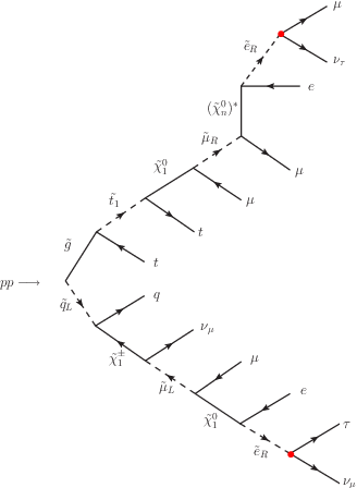
In general, more complicated SUSY production and decay processes than Eq. (15) can occur. Fig. 4 gives an example of (left-handed) squark-gluino production followed by two lengthy decay chains. Typically, these processes lead to additional final state particles [compared to Eq. (15) and Table 3], most notably

•

additional jets from the production of gluinos and their subsequent decays into squarks and quarks; cf. the upper decay chain of Fig. 4,
•

additional leptons from the decays of heavier neutralinos and charginos, which may come from the decay of left-handed squarks, like in the lower decay chain of Fig. 4, and
•

additional leptons from a ${\tilde{\chi}}^{0}_{1}$ decay into a non-LSP right-handed slepton $\tilde{\ell}^{\prime}_{R}$ (or lightest stau ${\tilde{\tau}}_{1}$ ), e.g. ${\tilde{\chi}}^{0}_{1}\to\ell^{\prime-}\tilde{\ell}^{\prime+}_{R}$ , followed by the three-body decay $\tilde{\ell}^{\prime+}_{R}\to\ell^{\prime+}\ell^{\pm}\tilde{\ell}_{R}^{\mp}$ via a virtual neutralino, $({\tilde{\chi}}^{0}_{n})^{*}$ ; see the upper decay chain of Fig. 4 for an example. Here, $\tilde{\ell}_{R}$ is the LSP.

These three-body slepton decays are special to $\tilde{e}_{R}$ and $\tilde{\mu}_{R}$ LSP scenarios. The corresponding decay rates are calculated in Appendix D and are taken into account in the following collider analysis.

The coupling $\mathbf{\Lambda}$ in $\tilde{\ell}_{R}$ LSP scenarios is of similar size as the gauge couplings and thus enables $R$ -parity violating decays with a significant branching ratio of sparticles which are not the LSP. Thus, not every SUSY decay chain involves the LSP. Of particular importance are the 2-body $R$ -parity violating decays of the ${\tilde{\tau}}_{1}$ [16], especially in the case when a ${\tilde{\tau}}_{1}$ NLSP is nearly mass degenerate with the $\tilde{\ell}_{R}$ LSP, like for the benchmark point BE1; cf. Table 7. Furthermore, sneutrinos (left-handed charged sleptons) may decay into two hard charged leptons (one charged lepton and a neutrino) if they couple directly to the dominant $R$ -parity violating operator. This leads to a sharp sneutrino mass peak in the respective dilepton invariant mass distribution as we will show in Sec. V. From the $R$ -parity violating left-handed slepton decays we expect large amounts of missing energy from the neutrino.

The lightest top squark, $\tilde{t}_{1}$ , is in most ${\mathrm{B}_{\,\!3}}$ mSUGRA scenarios the lightest squark. Thus, $\tilde{t}_{1}$ pair production forms a sizable fraction of all SUSY production processes. The decay of each $\tilde{t}_{1}$ yields at least one $b$ -quark (either directly from the decay $\tilde{t}_{1}\to\tilde{\chi}_{1}^{+}b$ and/or from the top quark decay after $\tilde{t}_{1}\to{\tilde{\chi}}^{0}_{1}t$ ). We therefore expect an enhanced $b$ -quark multiplicity for $\tilde{t}_{1}$ pair production. We will use the $b$ -quark multiplicity in Sec. V to discriminate these events from other SUSY processes.

To conclude this discussion, as one can see from Table 3, we expect multi-lepton final states for $\tilde{e}_{R}$ and $\tilde{\mu}_{R}$ LSP scenarios at the LHC. One the one hand, we obtain charged leptons from the ${\tilde{\chi}}^{0}_{1}$ decay into the $\tilde{\ell}_{R}$ LSP. On the other hand, each LSP decay involves a charged lepton. Furthermore, as explained above, also non LSPs can decay via the dominant $R$ -parity violating operator into leptons. Therefore, a multi-lepton analysis will be the best search strategy for our $\tilde{\ell}_{R}$ LSP scenarios.

Multi charged lepton final states (especially electrons and muons) are one of the most promising signatures to be tested with early LHC data. Electrons and muons can be easily identified and the SM background for high lepton multiplicities is very low [17]. We therefore investigate in the following the discovery potential of $\tilde{e}_{R}$ LSP scenarios with an inclusive three lepton search analysis. We will treat electrons and muons equally and thus expect similar results for $\tilde{\mu}_{R}$ LSP scenarios.

IV Discovery Potential at the LHC

In this section, we study the discovery potential of $\tilde{e}_{R}$ and $\tilde{\mu}_{R}$ LSP models with an inclusive search analysis for tri-lepton final states at the LHC. Because of the striking multi-leptonic signature of these models (see Sec. III), a discovery might be possible with early LHC data. We therefore study the prospects at the LHC assuming separately a center-of-mass system (cms) energy of $7\mbox{~TeV}$ and $14\mbox{~TeV}$ .

IV.1 Major Backgrounds

In the following Monte Carlo (MC) study, we consider SM backgrounds that can produce three or more charged leptons (electrons or muons) in the final state at the particle level, i.e. after (heavy flavor) hadron and tau lepton decays. For the heavy flavor quarks, we consider bottom, $b$ , and charm, $c$ , quarks [88]. Moreover, we expect the SUSY signal events to contain additional energy from hard jets arising from decays of the heavier (colored) sparticles. We thus consider the following SM processes as the major backgrounds in our analysis:

•

Top production. We consider top pair production ( $t\overline{t}$ ), single-top production associated with a $W$ boson ( $Wt$ ) and top pair production in association with a gauge boson ( $Wt\overline{t}$ , $Zt\overline{t}$ ). Each top quark decays into a $W$ boson and a $b$ quark. Leptons may then originate from the $W$ and/or $b$ decay.
•

$Z+\mbox{jets}$ , i.e. $Z$ boson production in association with one or two (parton level) jets. For the associated jet(s) we consider only $c$ - and $b$ -quarks. We force the $Z$ boson to decay leptonically.
•

$W+\mbox{jets}$ , i.e. $W$ boson production in association with two heavy flavor quarks ( $c$ or $b$ ) at parton level. We demand that the $W$ decays into a charged lepton and a neutrino.
•

Di-boson ( $WZ$ , $ZZ$ ) and di-boson $+$ jet ( $WWj$ , $WZj$ , $ZZj$ ) production. For the $WZ$ and $ZZ$ background, the gauge bosons are forced to decay leptonically. For $WWj$ , we consider only the heavy flavor quarks $c$ and $b$ for the (parton level) jet, while for $WZj$ and $ZZj$ every quark flavor is taken into account.

We have also included the processes, where we have a virtual gamma instead of a $Z$ boson.

Sample	Sub-sample	LO cross section [pb]		Simulated events		Generator
		$7\mbox{~TeV}$	$14\mbox{~TeV}$	$7\mbox{~TeV}$	$14\mbox{~TeV}$
top	$t\overline{t}$	$86.7$	$460$	$200~000$	$5~000~000$	Herwig
	$Wt$	$10.2$	$60.7$	$100~000$	$1~200~000$	MadGraph + Herwig
	$Wt\overline{t}$	$0.14$	$0.52$	$10~000$	$10~000$	MadGraph + Herwig
	$Zt\overline{t}$	$0.066$	$0.43$	$10~000$	$10~000$	Herwig
$Z+\mbox{jets}$	$Zc\overline{c}$	$49.5$	$187$	$100~000$	$2~000~000$	Herwig
	$Zb\overline{b}$	$44.6$	$171$	$100~000$	$2~000~000$	Herwig
	$Z(\to\ell^{+}\ell^{-})+j\,\,(j=c,b)$	$59.6$	$203$	$180~000$	$3~700~000$	MadGraph + Herwig
$W+\mbox{jets}$	$W(\to\ell\nu)+jj\,\,(j=c,b)$	$38.2$	$95.2$	$135~000$	$1~400~000$	MadGraph + Herwig
di-boson	$WZ\to\mbox{leptons}$	$0.20$	$0.40$	$100~000$	$100~000$	MadGraph + Herwig
	$ZZ\to\mbox{leptons}$	$0.03$	$0.06$	$22~000$	$75~000$	MadGraph + Herwig
	$WW+j\,\,(j=c,b)$	$10.9$	$64.0$	$120~000$	$1~000~000$	MadGraph + Herwig
	$WZ+j\,\,(j=\mbox{all flavors})$	$7.0$	$25.0$	$77~000$	$100~000$	MadGraph + Herwig
	$ZZ+j\,\,(j=\mbox{all flavors})$	$3.2$	$10.2$	$16~000$	$280~000$	MadGraph + Herwig

Table 4: SM background MC samples (first and second column) used for our analysis. The third and fourth (fifth and sixth) column shows the leading-order cross section (number of simulated events) for

pp

collisions at a cms energy of

\sqrt{s}=7\mbox{~TeV}

and

\sqrt{s}=14\mbox{~TeV}

, respectively. For the event simulation we employ the MC generator listed in the last column. We also have included the processes, where we have a virtual gamma instead of a

Z

boson.

For the backgrounds with heavy flavor quarks, we demand (at parton level) a minimal transverse momentum for the $c$ or $b$ quarks of $p_{T}\geq 10\mbox{~GeV}$ corresponding to our object selection cut for the leptons, cf. Sec. IV.2. Table 4 gives an overview of the background samples used in our analysis. In principle, QCD production of four heavy flavor quarks, like $b\bar{b}b\bar{b}$ production, can also produce three lepton events. However, these backgrounds are negligible compared to the other backgrounds in Table 4, because the probability of obtaining three isolated leptons from heavy flavor decay is too low [89].

IV.2 Monte Carlo Simulation and Object Selection

The $t\overline{t}$ , $Zt\overline{t}$ , $Zc\overline{c}$ and $Zb\overline{b}$ backgrounds are simulated with Herwig6.510 [90, 91, 92]. For the other SM processes we employ MadGraph4.4.30 [93] for the generation of the hard process which is then fed into Herwig. The employed MC generators are listed in Table 4. We also give the leading-order (LO) cross section and the number of simulated events for each background sample for both cms energies. The cross sections are taken from Herwig (for the $t\overline{t}$ , $Zt\overline{t}$ , $Zc\overline{c}$ and $Zb\overline{b}$ backgrounds) or MadGraph (else). We only consider the leading-order cross sections for the signal and background samples. We note however that the next-to-leading-order (NLO) corrections can be large, see e.g. Refs. [94, 95, 96, 97, 98], and should be included in a more dedicated analysis. Furthermore, our simulation does not account for detector effects, i.e. we neglect backgrounds with leptons faked by jets or photons. However, we expect these backgrounds to be small, because the fake rate for electrons and muons is quite low [17].

The SUSY mass spectra were calculated with SOFTSUSY3.0.13 [74, 75]. The SOFTSUSY output was then fed into ISAWIG1.200 and ISAJET7.64 [99] in order to calculate the decay widths of the SUSY particles. We added the missing three-body slepton decays $\tilde{\ell}^{\prime}_{R}\to\ell^{\prime}\ell\tilde{\ell}_{R}$ and $\tilde{\tau}_{1}\to\tau\ell\tilde{\ell}_{R}$ to the ISAJET code; see Appendix D for the calculation and a discussion of these new slepton decays. The signal processes, i.e. pair production of all SUSY particles, were simulated with Herwig6.510.

Production process	Cross section [fb] at $\sqrt{s}=7\mbox{~TeV}$			Cross section [fb] at $\sqrt{s}=14\mbox{~TeV}$
	BE1	BE2	BE3	BE1	BE2	BE3
$pp\to\mbox{sparton pairs}$	$86.7$	$152$	$139$	$1970$	$2770$	$2760$
$pp\to\mbox{slepton pairs}$	$24.0$	$19.9$	$21.1$	$96.7$	$83.9$	$88.1$
$pp\to\begin{array}[]{l}\mbox{gaugino pairs},\\ \mbox{gaugino+sparton}\end{array}$	$32.2$	$38.6$	$43.3$	$224$	$259$	$284$
$pp\to\mbox{sparticle pairs}$	$143$	$210$	$203$	$2290$	$3110$	$3130$

Table 5: Total LO cross section (in fb) for the benchmark scenarios BE1, BE2 and BE3 for pair production of all SUSY particles (last row) and three of its subprocesses: sparton (i.e. squark and gluino) pair production (second row), slepton pair production (third row) and electroweak (EW) gaugino pair or EW gaugino plus sparton production (fourth row). We separately assume

pp

collisions at cms energies of

\sqrt{s}=7\mbox{~TeV}

and

\sqrt{s}=14\mbox{~TeV}

. The cross sections are calculated with Herwig. We have simulated

\approx 15~000

(

\approx 250~000

) SUSY events for the

7\mbox{~TeV}

(

14\mbox{~TeV}

) MC signal sample.

We give in Table 5 leading order cross sections for sparticle pair production at the LHC for the three benchmark scenarios BE1, BE2 and BE3, cf. Table 2. We separately assume cms energies of $\sqrt{s}=7\mbox{~TeV}$ and $\sqrt{s}=14\mbox{~TeV}$ . We present the cross sections for the signal (last row), i.e. pair production of all sparticles, and for three of its subprocesses: The production of sparton pairs (second row), where we consider squarks and gluinos as spartons, slepton pair production (third row) and the production of electroweak (EW) gaugino pairs or an EW gaugino in association with a squark or gluino (fourth row). For all benchmark points, sparton pair production is the dominant SUSY production process. Therefore, the majority of the SUSY events will fulfill our signature expectations including at least two hard jets, cf. Sec. III.

For the reconstruction of jets, we employ FastJet 2.4.1 [100, 101] using the kt-algorithm with cone radius $\Delta R=0.4$ . Here $\Delta R\equiv\sqrt{(\Delta\phi)^{2}+(\Delta\eta)^{2}}$ , where $\eta$ ( $\phi$ ) is the pseudorapidity (azimuthal angle). We only select jets and leptons (i.e. electrons and muons) if $|\eta|<2.5$ and if their transverse momentum is larger than $10\mbox{~GeV}$ . In addition, leptons are rejected, if the total transverse momentum of all particles within a cone of $\Delta R<0.2$ around the lepton three-momentum axis exceeds $1\mbox{~GeV}$ .

IV.3 Kinematic Distributions

In this section we discuss kinematic distributions for the benchmark points of Table 2 and motivate our cuts of Sec. IV.4. The distributions correspond to our $7\mbox{~TeV}$ event sample and are normalized to one.

The $p_{T}$ distribution of all electrons [muons] after object selection (cf. the last paragraph of Sec. IV.2) is shown in Fig. 5(a) [Fig. 5(b)] for the ${\mathrm{B}_{\,\!3}}$ mSUGRA benchmark models BE1, BE2 and BE3. In all scenarios, the electrons mostly stem from the neutralino decay ${\tilde{\chi}}^{0}_{1}\to\tilde{e}_{R}e$ , while many of the muons come from the LSP decay $\tilde{e}_{R}\to\mu\nu_{\tau}$ , cf. Appendix A.

We observe in Fig. 5(a) that BE1 leads to the in average hardest electrons. In this scenario, the mass difference between the ${\tilde{\chi}}^{0}_{1}$ (decaying often via ${\tilde{\chi}}^{0}_{1}\to e\tilde{e}_{R}$ ) and the $\tilde{e}_{R}$ LSP is about 27 GeV and thus quite large (compared to the other benchmark points). Furthermore, the ${\tilde{\tau}}_{1}$ NLSP decays dominantly via the $R$ -parity violating decay ${\tilde{\tau}}_{1}\to e\nu_{\mu}$ . A large fraction of the ${\tilde{\tau}}_{1}$ mass is thus transformed into the 3-momentum of an electron. From both sources, we obtain electrons with large $p_{T}$ . For example, $81\%$ of all selected electrons have $p_{T}^{\mathrm{el}}\gtrsim 25\mbox{~GeV}$ in BE1.

The situation for BE2 and BE3 is different. Because of the smaller mass difference between the ${\tilde{\chi}}^{0}_{1}$ and the $\tilde{e}_{R}$ LSP (compared to BE1), the electrons from ${\tilde{\chi}}^{0}_{1}$ decay are less energetic. For instance, the fraction of selected electrons with $p_{T}^{\mathrm{el}}\lesssim 25\mbox{~GeV}$ is $55\%$ ( $34\%$ ) for BE2 (BE3). Furthermore, the electron multiplicity is reduced in these scenarios, because many electrons fail the lower $p_{T}$ cut ( $p_{T}^{\mathrm{el}}>10\mbox{~GeV}$ ) of the object selection. Due to this, $30\%$ ( $50\%$ ) of all events do not contain any selected electron in BE2 (BE3).

In contrast, the situation for the muons, Fig. 5(b), is reversed (compared to the electrons). A large amount of the muons are soft in BE1, whereas BE2 and BE3 have a harder muon $p_{T}$ spectrum. Note that for BE1, a sizable fraction of all muons do not even fulfill the object selection requirement of $p_{T}>10\mbox{~GeV}$ , so that $34\%$ of all events do not contain any selected muon. These muons in BE1 stem, for example, from the 3-body decays of the $\tilde{\mu}_{R}$ into the $\tilde{e}_{R}$ or the ${\tilde{\tau}}_{1}$ and are in general soft due to decreased phase space, cf. Table 7. In contrast, the muons in BE2 and BE3 are on average much harder, since the majority of these muons originate from the $\tilde{e}_{R}$ LSP decay.

We conclude, that the lepton $p_{T}$ spectrum strongly depends on the sparticle mass spectrum. Therefore, we desist from making further requirements on the lepton $p_{T}$ since this would imply a strong model dependence in the event selection. We will only require at least three charged (and isolated) leptons as one of our cuts in the next section.

We show in Fig. 6(a) [Fig. 6(b)] the $p_{T}$ distribution of the [second] hardest jet for the benchmark points BE1, BE2 and BE3. For all scenarios, we observe a broad peak of the hardest jet $p_{T}$ at around $400\mbox{~GeV}$ . Many of these jets stem from the decays of first and second generation squarks into the ${\tilde{\chi}}^{0}_{1}$ ; cf. Table 7–Tab 9.

We find another peak in Fig. 6(a) as well as in Fig. 6(b) at around $100\mbox{~GeV}$ . These jets stem mainly from the $t$ quark decay products from $\tilde{t}_{1}\to t{\tilde{\chi}}^{0}_{1}$ decay. The peak is most pronounced in BE2, since here we have a light $\tilde{t}_{1}$ mass, $M_{\tilde{t}_{1}}=448\mbox{~GeV}$ , and thus an enhanced $\tilde{t}_{1}$ pair production cross section. In contrast, the $\tilde{t}_{1}$ mass is about $80\mbox{~GeV}$ heavier in BE1 and therefore, the peak is hardly visible in Fig. 6.

For BE1, the $p_{T}$ distribution of the hardest and second hardest jet peaks at low values. These soft jets stem from initial and final state radiation. They appear as the hardest jets in EW gaugino and slepton pair production which forms a sizable fraction ( $39\%$ ) of all SUSY production processes in BE1, cf. Table 5. They are less important for BE2 and BE3. However, this picture will change for a cms energy of $\sqrt{s}=14\mbox{~TeV}$ , where sparton pair production is much more dominant in BE1.

Because most events possess at least two jets, we demand in the following section at least two jets as one of our cuts. Furthermore, we take into account that many jets (and some of the leptons) are hard, i.e. we demand the visible effective mass to be larger than a few 100 GeV; see the next section for details.

IV.4 Event Selection and Cutflow

We now develop a set of cuts in order to obtain a statistically significant signal and a good signal to (SM) background ratio. To motivate the different selection steps, we show in Fig. 7 the event distributions that correspond to the different cut variables before the respective cut is applied. We give distributions for the three $\tilde{e}_{R}$ LSP benchmark models (BE1, BE2, BE3), for the SM background, and, for comparison, for the $R$ -parity conserving benchmark model SPS1a [51]⁵⁵ 5 SPS1a has a mass spectrum similar to BE1, BE2, and BE3. The main difference lies in the light part of the spectrum, where we have in SPS1a a stable and invisible ${\tilde{\chi}}^{0}_{1}$ LSP. The ${\tilde{\tau}}_{1}$ is the NLSP. Furthermore, the overall mass scale is a bit lower, e.g. the squark and gluino masses are around 500-600 GeV.. The distributions correspond to an integrated luminosity of 1 fb^-1 at $\sqrt{s}=7\mbox{~TeV}$ .

Sample	Before cuts	$N_{\mathrm{lep}}\geq 3$	$N_{\mathrm{jet}}\geq 2$	$M_{\mathrm{OSSF}}$	$M_{\mathrm{eff}}^{\mathrm{vis}}\geq 300\mbox{~GeV}$
top	$97111\pm 197$	$14.9\pm 2.2$	$13.8\pm 2.1$	$12.0\pm 2.1$	$2.1\pm 0.8$
$Z+\mbox{jets}$	$153591\pm 254$	$51.9\pm 4.3$	$16.6\pm 2.4$	$1.0\pm 0.6$	$\lesssim 1.0$
$W+\mbox{jets}$	$38219\pm 103$	$\lesssim 1.0$	$\lesssim 1.0$	$\lesssim 1.0$	$\lesssim 1.0$
di-boson	$21331\pm 48$	$179.2\pm 3.0$	$53.5\pm 2.0$	$2.6\pm 0.4$	$0.7\pm 0.2$
all SM	$310252\pm 341$	$264.0\pm 5.7$	$83.9\pm 3.8$	$15.6\pm 2.2$	$2.8\pm 0.8$
BE1	$143.1\pm 1.2$	$90.5\pm 0.9$	$79.4\pm 0.9$	$68.8\pm 0.8$	$65.5\pm 0.8$
$S/\sqrt{B}$	-	$5.6$	$8.7$	$17.4$	$39.1$
BE2	$210.4\pm 1.5$	$92.6\pm 1.0$	$81.4\pm 0.9$	$73.8\pm 0.9$	$70.4\pm 0.8$
$S/\sqrt{B}$	-	$5.7$	$8.9$	$18.7$	$42.1$
BE3	$202.7\pm 1.4$	$61.6\pm 0.8$	$51.3\pm 0.7$	$45.2\pm 0.7$	$43.2\pm 0.7$
$S/\sqrt{B}$	-	$3.8$	$5.6$	$11.4$	$25.8$

Table 6: Number of SM background and signal events after each step in the event selection corresponding to an integrated luminosity of

1~\mathrm{fb}^{-1}

\sqrt{s}=7\mbox{~TeV}

. For each signal model (BE1, BE2 and BE3, see Table 2), we show

S/\sqrt{B}

as significance estimator. The uncertainties correspond to statistical fluctuations.

In Table 6, we give the number of background and signal events after each cut of the analysis. Furthermore, we provide for each signal benchmark scenario the significance estimator $S/\sqrt{B}$ , where $S$ ( $B$ ) is the number of signal (SM background) events. In general, the signal can be defined to be observable if [52]

\displaystyle S\geq max\left[5\sqrt{B},~5,~0.5B\right].

(16)

The requirement $S\geq 0.5B$ avoids the possibility that a small signal on top of a large background could otherwise be regarded as statistically significant, although this would require the background level to be known to an excellent precision. In the case of a very low background expectation, $B<1$ , we still require $5$ signal events for a discovery.

As we have seen in Sec. III, we expect an extensive number of charged leptons in the final state. However, the lepton flavor multiplicity, i.e. the multiplicity of electrons and muons, depends strongly on the LSP flavor as well as on the dominant $\mathbf{\Lambda}$ coupling, cf. Table 3. In addition, as we have seen in the last section, the $p_{T}$ spectrum of the leptons is strongly correlated to the details of the mass hierarchy. Therefore, in order to be as model independent as possible, we simply demand as our first cut three charged leptons (electrons or muons) in the final state without further requirements on the $p_{T}$ (beside the object selection cut of $p_{T}>10\mbox{~GeV}$ ).

How useful this cut is, can be seen in Fig. 7(a), where we show the lepton multiplicity after object selection cuts. The distribution for the $\text{B}_{3}$ benchmark scenarios peaks around 2-3 leptons, whereas most of the SM background events posses less than three electrons or muons. In principle, by demanding at least five charged leptons in the final state, we can already get a (nearly) background free event sample. However, such a cut would also significantly reduce the number of signal events and is therefore less suitable for an analysis of early data. We also observe in Fig. 7(a) many more leptons in the $R$ -parity violating scenarios than in SPS1a. This is expected, due to the additional leptons from the decays of and into the selectron LSP.

As can be seen in the third column of Table 6, after demanding three leptons, the main SM background comes from di-boson events. They account for $68\%$ of the background. Furthermore, no $W+\mbox{jets}$ events survive this cut, indicated by “ $\lesssim 1.0$ ” events in the fourth row of Table 6. At the same time, the number of signal events is reduced to $63\%$ , $44\%$ and $30\%$ for BE1, BE2 and BE3, respectively. Because of the low mass difference between the ${\tilde{\chi}}^{0}_{1}$ and the $\tilde{e}_{R}$ LSP in BE3, many electrons from ${\tilde{\chi}}^{0}_{1}$ decay fail the object selection cuts; cf. the discussion of Fig. 5(a). BE1 and BE2 might already be observable after the first cut, i.e. $S/\sqrt{B}>5$ .

Next, we will use the fact that we expect several jets from squark and gluino decays; see Sec. III. The jet multiplicity after demanding three leptons is shown in Fig. 7(b). Because of the weak object selection criteria for the jets ( $p_{T}>10\mbox{~GeV}$ ) and the small radius for the jet reconstruction ( $\Delta R=0.4$ ), we observe a high jet multiplicity. As discussed in Sec. III, we expect at least two jets from squark and gluino decays. Therefore we demand as our second cut (fourth column of Table 6) the number of jets to be larger than two, i.e. $N_{\mathrm{jet}}\geq 2$ . This cut suppresses roughly two thirds of the di-boson backgrounds $WZ$ and $ZZ$ as well as of the $Z+\mbox{jets}$ background. However, di-boson production, especially $WZ+j$ , still accounts for most of the background. The number of signal events is only reduced by 12%-17%. After this cut, all our benchmark points fulfill the criteria in Eq. (16) and are thus observable.

In order to further reduce the SM backgrounds involving $Z$ bosons, we construct all possible combinations of the invariant mass of opposite-sign-same-flavor (OSSF) leptons. The distributions (after the three lepton and $N_{\mathrm{jet}}\geq 2$ cut) are shown in Fig. 7(c). As expected, the SM background has a large peak at the $Z$ boson mass $M_{Z}=91.2\mbox{~GeV}$ , while the signal distribution is mostly flat in that region. Thus as our third cut (fifth column of Table 6) of our event selection, we reject all events where the invariant mass of at least one OSSF lepton pair lies within a $10\mbox{~GeV}$ window around the $Z$ boson mass, i.e. we demand

\displaystyle M_{\mathrm{OSSF}}\not\in\left[81.2\mbox{~GeV},101.2\mbox{~GeV}\right].

(17)

This cut strongly reduces the $Z+\mbox{jets}$ and di-boson backgrounds, leaving $t\overline{t}$ as the dominant SM background. Roughly $90\%$ of the signal events (for all benchmark scenarios) survive this cut. The statistical significance now lies between 10 and 20 for all benchmark points.

As we have shown in Sec. IV.3, our SUSY events contain a large amount of energy in the form of high- $p_{T}$ jets and leptons. Thus, we construct the visible⁶⁶ 6 We denote this variable as visible effective mass because it does not include the missing transverse energy as in other definitions of the effective mass [17]. effective mass,

\displaystyle M_{\mathrm{eff}}^{\mathrm{vis}}\equiv\sum_{i=1}^{4}p_{T}^{\mathrm{jet},i}+\sum_{\mathrm{all}}p_{T}^{\mathrm{lep}},

(18)

i.e. the scalar sum of the absolute value of the transverse momenta of the four hardest jets and all selected leptons in the event. The visible effective mass distribution is shown in Fig. 7(d). The SM background dominates for $M_{\mathrm{eff}}^{\mathrm{vis}}<300\mbox{~GeV}$ , while most of the signal events exhibit a visible effective mass above $300\mbox{~GeV}$ . This value is slightly higher for the $14\mbox{~TeV}$ dataset. Therefore, we demand as our last cut of our event selection (last column of Table 6)

\displaystyle M_{\mathrm{eff}}^{\mathrm{vis}}>\left\{\begin{array}[]{l}300\mbox{~GeV},\quad\mbox{if}\,\sqrt{s}=7\mbox{~TeV},\\ 400\mbox{~GeV},\quad\mbox{if}\,\sqrt{s}=14\mbox{~TeV}.\end{array}\right.

After this cut, only $2.8\pm 0.8$ SM events remain at $\sqrt{s}=7\mbox{~TeV}$ and an integrated luminosity of 1 fb^-1. The background is dominated by $t\overline{t}$ production. The signal is nearly unaffected by this cut as can be seen in Table 6. The statistical significance is now roughly as large as 25 (40) for the benchmark point(s) BE3 (BE1 and BE2). Furthermore, the signal to background ratio is now of $\mathcal{O}(10)$ . Therefore, systematic uncertainties of the SM backgrounds are not problematic. A signal is clearly visible.

We observe in Fig. 7(d) two peaks in the visible effective mass distributions for our benchmark scenarios. The peak at lower values of $M_{\mathrm{eff}}^{\mathrm{vis}}$ contains mainly events from $\tilde{t}_{1}$ pair production, while events from (right-handed) first and second generation squark or gluino production build the second peak at higher $M_{\mathrm{eff}}^{\mathrm{vis}}$ values. Because of the large mass difference between the $\tilde{t}_{1}$ and the other squarks of about $400\mbox{~GeV}-500\mbox{~GeV}$ (depending on the model, see Table 7-Table 9), these peaks are clearly separated in the visible effective mass. We make use of this fact in Sec. V when we present a method to reconstruct the masses of both the $\tilde{t}_{1}$ and the right-handed first and second generation squarks.

In order to test the flavor sensitivity of our analysis, we have applied our cuts to a modified version of the benchmark models presented in Table 2. Instead of ${\bf\lambda}_{231}$ , we chose ${\bf\lambda}_{131}$ ( ${\bf\lambda}_{132}$ ) as the dominant $R$ -parity coupling at $M_{\rm GUT}$ to obtain the $\tilde{e}_{R}$ ( $\tilde{\mu}_{R}$ ) as the LSP, while leaving the other ${\mathrm{B}_{\,\!3}}$ mSUGRA parameters unchanged. The results for the $\tilde{\mu}_{R}$ LSP scenarios are in agreement with the original benchmark scenarios within statistical fluctuations of the MC samples.

However, for the $\tilde{e}_{R}$ LSP scenarios with a dominant ${\bf\lambda}_{131}$ coupling at $M_{\rm GUT}$ , the cut on the invariant mass of OSSF leptons rejects more signal events than for scenarios with ${\bf\lambda}_{231}$ . For the modified scenario of BE1 (BE2), the number of signal events passing the $M_{\mathrm{OSSF}}$ cut is reduced by around $15\%$ ( $3\%$ ) compared to the original results, cf. Table 6. This difference is strongest for BE1–like scenarios, because the endpoint of the di-electron invariant mass distribution, where one electron comes from the ${\tilde{\chi}}^{0}_{1}$ decay and the other from the $\tilde{e}_{R}$ LSP decay, cf. also Eq. (26a), coincides with the upper value of the $Z$ boson mass window. However, this is just a coincidence and a different mass spectrum (compared to BE1) with a $\tilde{e}_{R}$ LSP and ${\bf\lambda}_{131}$ at $M_{\rm GUT}$ will not have such a suppression.

We conclude that in most cases, our detailed study of $\tilde{e}_{R}$ LSP models with a dominant $R$ -parity violating coupling ${\bf\lambda}_{231}$ is representative for all ${\mathrm{B}_{\,\!3}}$ mSUGRA models with a $\tilde{e}_{R}$ or $\tilde{\mu}_{R}$ LSP.

To end this subsection, we present in Fig. 8 the missing transverse energy, $\hbox to0.0pt{\hbox to7.95831pt{\hfil/\hfil}\hss}E_{T}$ , distribution for the benchmark scenarios, for SPS1a and for the combined SM backgrounds before any cuts are applied. In $R$ -parity conserving scenarios like SPS1a, the ${\tilde{\chi}}^{0}_{1}$ LSP is stable and escapes detection leading to large amounts of $\hbox to0.0pt{\hbox to7.95831pt{\hfil/\hfil}\hss}E_{T}$ . However, for our benchmark points, even though the $\tilde{e}_{R}$ LSP decays within the detector, we observe a significant amount of missing energy due to the neutrinos from the LSP decay. Moreover, the $\hbox to0.0pt{\hbox to7.95831pt{\hfil/\hfil}\hss}E_{T}$ distribution for SPS1a falls off more rapidly than in the ${\mathrm{B}_{\,\!3}}$ scenarios. This is because the neutrinos are quite hard, resulting from a 2–body decay with a large mass difference. Thus, ${\mathrm{B}_{\,\!3}}$ scenarios can lead to even more missing transverse energy than $R$ -parity conserving scenarios. We have not employed $\hbox to0.0pt{\hbox to7.95831pt{\hfil/\hfil}\hss}E_{T}$ in our analysis, because our simple cuts already sufficiently suppress the SM background. Furthermore, it is easier to reconstruct electrons and muons than missing energy, especially in the early stages of the experiments.

IV.5 Discovery Potential at the LHC

In this subsection, we extend our previous analysis. We perform a two dimensional parameter scan in the ${M_{1/2}}$ – $M_{0}$ plane around the benchmark point BE1 (Table 2). For each parameter point, we generate $1000$ signal events, i.e. the pair production of all SUSY particles. We then apply the same cuts developed in the previous section. We estimate the discovery potential of ${\mathrm{B}_{\,\!3}}$ mSUGRA models with a $\tilde{e}_{R}$ LSP for the early LHC run at $\sqrt{s}=7\mbox{~TeV}$ and also give prospects for the design energy of $\sqrt{s}=14\mbox{~TeV}$ .

Due to the RGE running, all sparticle masses at the weak scale, especially those of the strongly interacting sparticles, increase with increasing ${M_{1/2}}$ [86, 87]. Thus, by varying ${M_{1/2}}$ , we can investigate the discovery potential as a function of the SUSY mass scale. Furthermore, as we have seen in the previous two sections, the discovery potential is quite sensitive to the mass hierarchy of the lighter sparticles and, in particular, to the mass difference between the ${\tilde{\chi}}^{0}_{1}$ and the $\tilde{e}_{R}$ LSP. Increasing $M_{0}$ increases the masses of the scalar particles, while the gaugino masses are nearly unaffected. Thus, $M_{0}$ provides a handle to control the mass difference between the ${\tilde{\chi}}^{0}_{1}$ and the $\tilde{e}_{R}$ (or $\tilde{\mu}_{R}$ ) LSP.

We show in Fig. 9(a) the signal cross section (in pb) for the LHC with $\sqrt{s}=7\mbox{~TeV}$ and in Fig. 9(b) the respective signal efficiency, i.e. the fraction of signal events that pass our cuts. The results are given only for models with a $\tilde{e}_{R}$ LSP, while models with a ${\tilde{\chi}}^{0}_{1}$ LSP ( ${\tilde{\tau}}_{1}$ LSP) are indicated by the striped (checkered) region. The solid gray region (lower left corner of Fig. 9) is excluded by the experimental bound on the ${\bf\lambda}_{231}$ coupling, cf. Tab 1.

The signal cross section, Fig. 9(a), which is dominated by the production of colored sparticles, clearly decreases with increasing ${M_{1/2}}$ , i.e. with an increasing SUSY mass scale. For instance, increasing ${M_{1/2}}$ from $400\mbox{~GeV}$ to $500\mbox{~GeV}$ reduces the cross section from $0.6~\mathrm{pb}$ to $0.1~\mathrm{pb}$ , while the right-handed squark (gluino) mass increases from around $820\mbox{~GeV}$ ( $930\mbox{~GeV}$ ) to $1010\mbox{~GeV}$ ( $1150\mbox{~GeV}$ ). In contrast, the $M_{0}$ dependence of the signal cross section is negligible, over the small range it is varied.

For the benchmark scenario BE1, we find in Fig. 9(b) a signal efficiency of $46\%$ . Going beyond BE1, we observe that the signal efficiency lies between $30\%$ and $50\%$ for most of the $\tilde{e}_{R}$ LSP parameter space. Therefore, our analysis developed in Sec. IV.4 works also quite well for a larger set of $\tilde{e}_{R}$ LSP models.

However, the signal efficiency decreases dramatically if the mass difference, $\Delta M$ , between the ${\tilde{\chi}}^{0}_{1}$ and the $\tilde{e}_{R}$ LSP approaches zero. For models with $\Delta M\lesssim 2.5\mbox{~GeV}$ , the signal efficiency lies just around $10\%-20\%$ . As described in detail in Sec. IV.3, the electrons in this parameter region from the decay ${\tilde{\chi}}^{0}_{1}\to\tilde{e}_{R}e$ are usually very soft and thus tend to fail the minimum $p_{T}$ requirement of the object selection, i.e. $p_{T}>10\mbox{~GeV}$ . For models with $\Delta M>10\mbox{~GeV}$ , the signal efficiency becomes more or less insensitive to $\Delta M$ . Note that, if we choose a stronger minimum lepton $p_{T}$ requirement in our analysis, the band of low signal efficiency will become wider.

The signal efficiency depends also slightly on ${M_{1/2}}$ . At low values, ${M_{1/2}}\lesssim 400\mbox{~GeV}$ , i.e. for models with a light sparticle mass spectrum, more events are rejected by the cut on the visible effective mass. Moreover, the SM particles from cascade decays and LSP decays have in this case on average smaller momenta than in scenarios with a heavier mass spectrum, and thus may fail to pass the object selection⁷⁷ 7 However, due to our rather weak $p_{T}$ requirements for jets and leptons, this effect does not play a major role.. The signal efficiency is highest for values of ${M_{1/2}}$ between $450\mbox{~GeV}$ and $550\mbox{~GeV}$ and reaches up to $50\%$ . However, when going to very large ${M_{1/2}}$ , the signal efficiency again decreases. Here, the production of sparton pairs is suppressed due to their large masses and the jet multiplicity is reduced. Less events will then pass the $N_{\mathrm{jet}}\geq 2$ and $M_{\mathrm{eff}}^{\mathrm{vis}}$ cut. For example, for $M_{1/2}=500\mbox{~GeV}$ ( $M_{1/2}=700\mbox{~GeV}$ ), sparton pair production contributes (only) $58\%$ ( $24\%$ ) to the total sparticle pair production cross section.

We give in Fig. 10(a) the discovery potential of $\tilde{e}_{R}$ LSP scenarios at the LHC with $\sqrt{s}=7\mbox{~TeV}$ . The discovery reach for the integrated luminosities $100~\mathrm{pb}^{-1}$ , $500~\mathrm{pb}^{-1}$ and $1~\mathrm{fb}^{-1}$ is shown. We use Eq. (16) as criterion for a discovery. Furthermore, we present in Fig. 10(b) the signal to background ratio, $S/B$ , as a measure for the sensitivity on systematic uncertainties of the SM background. As shown in the previous section, the SM background is reduced to $2.8\pm 0.8$ events when we employ the cuts of Table 6.

Fig. 10(a) suggests that $\tilde{e}_{R}$ LSP scenarios up to ${M_{1/2}}\lesssim 620\mbox{~GeV}$ can be discovered with an integrated luminosity of $1~\mathrm{fb}^{-1}$ . This corresponds to squark masses of $1.2\mbox{~TeV}$ and $\tilde{e}_{R}$ LSP masses of around $230\mbox{~GeV}$ . For these models, we have a signal over background ratio of $S/B\approx 3$ and thus, systematic uncertainties of the SM background are not problematic. Furthermore, we see that BE1 ( $M_{1/2}=475$ GeV, $M_{0}=0$ GeV) can already be discovered with $\lesssim~100~\mathrm{pb}^{-1}$ of data. We also see in Fig. 10 that scenarios with a small mass difference between the ${\tilde{\chi}}^{0}_{1}$ and the $\tilde{e}_{R}$ LSP are more difficult to discover as expected from Fig. 9(b).

We now discuss the prospects of a discovery at the LHC at $\sqrt{s}=14\mbox{~TeV}$ . In Fig. 11(a), we give the signal cross section and in Fig. 11(b) the signal efficiency. We employ the cuts developed in Sec. IV.4. The cutflow at $\sqrt{s}=14\mbox{~TeV}$ for the benchmark scenarios can be found in Appendix B.

Because of the higher cms energy, the cross section is $\mathcal{O}(10)$ times larger than for $\sqrt{s}=7\mbox{~TeV}$ , cf. Fig. 9(a). For instance, at ${M_{1/2}}=400\mbox{~GeV}$ ( $500\mbox{~GeV}$ ) the signal cross section at $\sqrt{s}=14\mbox{~TeV}$ is now $7.2~\mathrm{pb}^{-1}$ ( $1.7~\mathrm{pb}^{-1}$ ). Furthermore, the signal, i.e. sparticle pair production, is now always dominated by sparton pair production, cf. also Table 5.

The signal efficiency at $\sqrt{s}=14\mbox{~TeV}$ is slightly improved compared to $\sqrt{s}=7\mbox{~TeV}$ . Because of the enhanced sparton pair production cross section, more signal events pass our cut on the jet multiplicity, $N_{\mathrm{jet}}\geq 2$ , cf. also Appendix B. We now obtain a signal efficiency of about $51\%$ (compared to $46\%$ at $\sqrt{s}=7$ TeV) for the benchmark point BE1. Most of the parameter points in Fig. 11(b) exhibit a signal efficiency in the range of $40\%$ to $60\%$ . For the scenarios with low mass difference between the ${\tilde{\chi}}^{0}_{1}$ and the $\tilde{e}_{R}$ LSP, $\Delta M\lesssim 2.5\mbox{~GeV}$ , the signal efficiency is reduced to around $15\%-25\%$ . As for $\sqrt{s}=7\mbox{~TeV}$ , the signal efficiency decreases at very large values of ${M_{1/2}}$ , because of the increasing sparton mass and the reduced sparton pair production cross section. Here, this effect slowly sets in at values ${M_{1/2}}\gtrsim 1100\mbox{~GeV}$ , i.e. for scenarios with squark and gluino masses around $2\mbox{~TeV}$ . However, even at ${M_{1/2}}=1100\mbox{~GeV}$ , sparton pair production still forms half of the total signal cross section.

We show in Fig. 12(a) the discovery potential for the LHC at $\sqrt{s}=14\mbox{~TeV}$ . We give the discovery reach for integrated luminosities of $100~\mathrm{pb}^{-1}$ , $1~\mathrm{fb}^{-1}$ and $10~\mathrm{fb}^{-1}$ , respectively. Our cuts of Sec. IV.4 reduce the SM background to $64.7\pm 7.2$ events for an integrated luminosity of $10~\mathrm{fb}^{-1}$ ; see Table 10. We observe that scenarios with ${M_{1/2}}\lesssim 1\mbox{~TeV}\,(1.15\mbox{~TeV})$ can be discovered with $1~\mathrm{fb}^{-1}$ ( $10~\mathrm{fb}^{-1}$ ). This corresponds to squark masses of around $1.9\mbox{~TeV}$ ( $2.2\mbox{~TeV}$ ) and LSP masses of roughly $370\mbox{~GeV}$ ( $450\mbox{~GeV}$ ). The respective signal over background ratio is $2$ ( $0.6$ ) as can be seen in Fig. 12(b). Therefore, systematic uncertainties of the SM background estimate are still not problematic as long as the SM events can be estimated to a precision of $\mathcal{O}(10\%)$ . This is a reasonable assumption after a few years of LHC running.

We conclude that due to the striking multi-lepton signature, the prospects of an early discovery of ${\mathrm{B}_{\,\!3}}$ mSUGRA with a $\tilde{\ell}_{R}$ LSP are better than for $R$ -parity conserving mSUGRA models [52]. Note that the vast reach in ${M_{1/2}}$ is also due to the typically light $\tilde{t}_{1}$ which has a large production cross section. For instance, at ${M_{1/2}}=525\mbox{~GeV}$ , the $\tilde{t}_{1}$ mass is around $630\mbox{~GeV}$ and thus can still be produced numerously at the LHC at $\sqrt{s}=7\mbox{~TeV}$ .

We want to remark that for scenarios with a low mass difference between the ${\tilde{\chi}}^{0}_{1}$ and the $\tilde{\ell}_{R}$ LSP, $\Delta M\lesssim 2.5\mbox{~GeV}$ , the search for like-sign di-lepton final states might be a more promising approach [52, 102, 103, 104]. However, a detailed analysis of these search channels is beyond the scope of this paper.

V Mass Reconstruction

We have shown in the previous section that large regions of the ${\mathrm{B}_{\,\!3}}$ mSUGRA parameter space with a $\tilde{\ell}_{R}$ LSP can already be tested with early LHC data. If a discovery has been made, the next step would be to try to determine the sparticle mass spectrum. We present now a strategy how the sparticle masses can be reconstructed. We use the benchmark point BE2 as an example. We assume an integrated luminosity of 100 fb^-1 and a cms energy of $\sqrt{s}=14\mbox{~TeV}$ in order to have enough events for the mass reconstruction.

The sparticle decay chains cannot be directly reconstructed, because the $\tilde{e}_{R}$ LSP decays always into an invisible neutrino. Thus, we focus on the measurement of edges and thresholds of invariant mass distributions which are a function of the masses of the involved SUSY particles. Our strategy is analogous to the one, that is widely used to reconstruct the mass spectrum in $R$ -parity conserving SUSY where a stable ${\tilde{\chi}}^{0}_{1}$ LSP escapes detection [105, 106, 107, 108, 109, 17].

V.1 The Basic Idea

We first discuss the general idea of the method. We assume the decay chain

\displaystyle D\to Cc\to Bbc\to Aabc,

(21)

illustrated in Fig. 13, where the particles $D$ , $C$ , $B$ , and $A$ are massive⁸⁸ 8 Particle $A$ does not necessarily need to be massive. In our case it is a massless neutrino. and their masses satisfy

\displaystyle m_{D}>m_{C}>m_{B}>m_{A}.

(22)

The particles $c$ , $b$ and $a$ are observable (massless) SM particles. Particle A is assumed to be invisible.

From the 4-momenta of the decay products $a$ , $b$ and $c$ , we can form the invariant mass combinations $m_{ba}$ , $m_{ca}$ , $m_{cb}$ and $m_{cba}$ . The maximal (denoted “max”) and minimal (denoted “min”) endpoints of these distributions,

\displaystyle m_{ba}^{\mathrm{max}},\,m_{ca}^{\mathrm{max}},\,m_{cb}^{\mathrm{max}},\,m_{cba}^{\mathrm{max}}\,\,\,\text{and}\,\,\,m_{cba}^{\mathrm{min}},

(23)

are functions of the (unknown) particle masses in Eq. (22)⁹⁹ 9 Another variable which can in principle be used for our scenarios is the Stransverse mass, $m_{T2}$ [110, 111, 108, 112, 113, 114].. The respective equations are given in Appendix C [115]. Note that $m_{ba}^{\mathrm{min}}$ , $m_{ca}^{\mathrm{min}}$ and $m_{cb}^{\mathrm{min}}$ are always equal to zero.

A prominent application of this method is the cascade decay of a left-handed squark in $R$ -parity conserving SUSY [17],

\displaystyle\tilde{q}_{L}\to q{\tilde{\chi}}^{0}_{2}\to q\ell_{n}^{\pm}\tilde{\ell}^{\mp}\to q\ell_{n}^{\pm}\ell_{f}^{\mp}{\tilde{\chi}}^{0}_{1}.

(24)

Here, the ${\tilde{\chi}}^{0}_{1}$ LSP is stable and escapes the detector unseen. Note that in $R$ -parity conserving SUSY, the “near” lepton, $\ell_{n}$ , and “far” lepton, $\ell_{f}$ , are of the same flavor and thus indistinguishable on an event-by-event basis. In our scenarios this is not necessarily the case, as shown below.

For our $\tilde{\ell}_{R}$ LSP scenarios, we investigate the decay chain of a right-handed squark, i.e.

\displaystyle\tilde{q}_{R}\to q{\tilde{\chi}}^{0}_{1}\to q\ell^{\pm}\tilde{\ell}_{R}^{\mp}\to q\ell^{\pm}\ell^{\prime\mp}\nu.

(25)

The LSP decays into a charged lepton $\ell^{\prime}$ and a neutrino, where the flavor depends on the dominant $\mathbf{{\bf\Lambda}}$ coupling, cf. Table 3. In contrast to the $R$ -parity conserving scenarios, we can actually distinguish the near and far lepton if we have $\mathbf{\Lambda}\in\{{\bf\lambda}_{231},{\bf\lambda}_{132}\}$ . The $\tilde{\ell}_{R}$ LSP then decays into a charged lepton of different flavor from its own. However, we still have to deal with combinatorial backgrounds, because we might wrongly combine leptons (and jets) from different cascades within the same event.

In the following, we demonstrate our method for the $\tilde{e}_{R}$ LSP benchmark model BE2 ( ${\bf\lambda}_{231}|_{\rm GUT}\not=0$ ), cf. Table 2. We focus on the case, where the $\tilde{e}_{R}$ LSP decays into a muon (instead of a $\tau$ ) and a neutrino. On the one hand, muons are much easier to reconstruct than $\tau$ leptons. On the other hand, muon events have a higher probability to pass our cuts, cf. Sect. IV.4. The relevant cascade decay, Eq. (25), is shown in Fig. 14. It yields one jet (at parton level) and two charged leptons of different flavor and opposite charge. From these objects, we can form the invariant masses $m_{e\mu}$ , $m_{\mu q}$ , $m_{eq}$ and $m_{e\mu q}$ .

In the mass determination, one can leave the mass of the neutrino as a free parameter. If one measures this parameter consistent with zero, it would be an important piece of information towards confirming our model. However, once the $R$ -parity violating decay chain of Fig. 14 is experimentally verified (or assumed), the knowledge of $m_{A}=0$ , Eq. (22), simplifies the equations in Appendix C and reduces the number of fit parameters by one. The endpoints of the invariant mass distributions are then given by


$\displaystyle(m_{e\mu}^{\mathrm{max}})^{2}=$	$\displaystyle M_{{\tilde{\chi}}^{0}_{1}}^{2}-M_{\tilde{e}_{R}}^{2},$	(26a)
$\displaystyle(m_{\mu q}^{\mathrm{max}})^{2}=$	$\displaystyle M_{\tilde{q}_{R}}^{2}-M_{{\tilde{\chi}}^{0}_{1}}^{2},$	(26b)
$\displaystyle(m_{eq}^{\mathrm{max}})^{2}=$	$\displaystyle(M_{\tilde{q}_{R}}^{2}-M_{{\tilde{\chi}}^{0}_{1}}^{2})(M_{{\tilde{\chi}}^{0}_{1}}^{2}-M_{\tilde{e}_{R}}^{2})/M_{{\tilde{\chi}}^{0}_{1}}^{2},$	(26c)
$\displaystyle(m_{e\mu q}^{\mathrm{max}})^{2}=$	$\displaystyle M_{\tilde{q}_{R}}^{2}-M_{\tilde{e}_{R}}^{2},$	(26d)
$\displaystyle(m_{e\mu q}^{\mathrm{min}})^{2}=$	$\displaystyle M_{\tilde{q}_{R}}^{2}(M_{{\tilde{\chi}}^{0}_{1}}^{2}-M_{\tilde{e}_{R}}^{2})/(2M_{{\tilde{\chi}}^{0}_{1}}^{2}).$	(26e)

In BE2 (and more generally in most $\tilde{\ell}_{R}$ LSP models within $\text{B}_{3}$ mSUGRA), the (mostly right-handed) $\tilde{t}_{1}$ is much lighter than the first and second generation $\tilde{q}_{R}$ . Therefore, we have typically two distinct squark mass scales. This enables a measurement of the $\tilde{t}_{1}$ and (first and second generation) $\tilde{q}_{R}$ mass simultaneously, if we are able to separate $\tilde{t}_{1}$ and $\tilde{q}_{R}$ production from each other¹⁰¹⁰ 10 From now on, $\tilde{q}_{R}$ stands only for right-handed squarks of the first and second generation.. This is possible as we show now.

V.2 Event Selection

For the mass reconstruction, we slightly extend our cuts developed in Sec. IV.4 for $\sqrt{s}=14\mbox{~TeV}$ . Each event has to contain at least one electron and one muon with opposite charge. In order to enhance the probability of selecting the right muon, i.e. the $\mu$ from the $\tilde{e}_{R}$ LSP decay, we require a minimal transverse momentum of the muon of $p_{T}^{\mu}\geq 25\mbox{~GeV}$ . We then construct all possible opposite-sign-different-flavor (OSDF) dilepton invariant masses, $m_{e\mu}$ , of electrons and muons (with $p_{T}^{\mu}\geq 25\mbox{~GeV}$ ). In order to reduce combinatorial backgrounds, we subtract the dilepton invariant mass distribution of the same-sign-different-flavor (SSDF) leptons. Note that this also suppresses (R-parity conserving) SUSY background processes, where the charges of the selected leptons are uncorrelated, because of an intermediate Majorana particle, i.e. a neutralino. For example, SUSY decay chains involving the cascade $\tilde{\mu}_{L}^{-}\to\mu^{-}{\tilde{\chi}}^{0}_{1}\to\mu^{-}e^{\pm}\tilde{e}_{R}^{\mp}$ are thus suppressed.

For the invariant mass distributions containing a jet, we design further selection cuts to discriminate between $\tilde{t}_{1}$ and $\tilde{q}_{R}$ events. We expect at least two $b$ jets in the $\tilde{t}_{1}$ events from the top quark decays. Thus, we introduce a simple $b$ -tagging algorithm in our simulation, assuming a $b$ -tagging efficiency of $60\%$ [17]. We demand two tagged $b$ jets for the $\tilde{t}_{1}$ event candidates while we require that no $b$ jet must be present for the $\tilde{q}_{R}$ event candidates. Moreover, we use the visible effective mass, $M_{\mathrm{eff}}^{\mathrm{vis}}$ , as a handle to discriminate between $\tilde{t}_{1}$ and $\tilde{q}_{R}$ events, i.e. we impose the cuts

\displaystyle\begin{array}[]{l}400\mbox{~GeV}\leq M_{\mathrm{eff}}^{\mathrm{vis}}\leq 900\mbox{~GeV}\quad\mbox{for $\tilde{t}_{1}$ events},\\ 900\mbox{~GeV}\leq M_{\mathrm{eff}}^{\mathrm{vis}}\quad\quad\quad\quad\quad\,\quad\mbox{for $\tilde{q}_{R}$ events},\end{array}

respectively.

For the construction of invariant mass distributions involving quarks, we consider the hardest and second hardest jet, $j_{1}$ and $j_{2}$ in each event, respectively. Due to the lighter $\tilde{t}_{1}$ mass, the jets are expected to be somewhat softer in $\tilde{t}_{1}$ events than in $\tilde{q}_{R}$ events. Therefore, for BE2, we choose the following $p_{T}$ selection criteria for the jets:

\displaystyle\begin{array}[]{l}\begin{array}[]{l}50\mbox{~GeV}\leq p_{T}^{j_{1}}\leq 250\mbox{~GeV}\\ 25\mbox{~GeV}\leq p_{T}^{j_{2}}\end{array}\Big\}\quad\mbox{for $\tilde{t}_{1}$ events},\\ \\ \begin{array}[]{l}250\mbox{~GeV}\leq p_{T}^{j_{1}}\\ 100\mbox{~GeV}\leq p_{T}^{j_{2}}\end{array}\Big\}\quad\mbox{for $\tilde{q}_{R}$ events}.\end{array}

The invariant mass distributions $m_{e\mu q}$ , $m_{eq}$ , and $m_{\mu q}$ are now constructed as follows:

•

$m_{e\mu q}$ : We take the invariant masses of the opposite sign electron and muon with $j_{1}$ and $j_{2}$ . The smaller (larger) value is taken for the edge (threshold) distribution. Note that we repeat this procedure for all possible combinations of electrons and muons. For the threshold distribution, we demand in addition the dilepton invariant mass to lie within $m_{e\mu}^{\mathrm{max}}/\sqrt{2}\leq m_{e\mu}\leq m_{e\mu}^{\mathrm{max}}$ , corresponding to the subset of events in which the angle between the two leptons (in the center of mass frame of the $\tilde{e}_{R}$ LSP) is greater than $\pi/2$ [105]. In the edge distribution, we require $m_{e\mu}\leq m_{e\mu}^{\mathrm{max}}$ and employ SSDF subtraction to reduce the combinatorial background.
•

$m_{eq}$ ( $m_{\mu q}$ ): We construct the invariant mass of all selected electrons (muons with $p_{T}^{\mu}\geq 25\mbox{~GeV}$ ) with $j_{1}$ and $j_{2}$ and take the lower value¹¹¹¹ 11 Here, we make use of the fact that we can distinguish the near and far lepton. However, we have checked that the model-independent construction of the variables $m_{\ell q(near/far)}$ as proposed in Ref. [105] leads to similar results.. Furthermore, we require $m_{e\mu}\leq m_{e\mu}^{\mathrm{max}}$ .

For these constructions, the dilepton invariant mass edge, $m_{e\mu}^{\mathrm{max}}$ , must have already been fitted. We use the true value of the dilepton edge, because it can be reconstructed to a very high precision, cf. Sec. V.3.1.

V.3 Results

We now show our results for BE2 for an integrated luminosity of $100~\mathrm{fb}^{-1}$ at $\sqrt{s}=14\mbox{~TeV}$ . We assume, that the SM background can be reduced to a negligible amount (cf. Appendix B) and present only the invariant mass distributions for the SUSY sample, i.e. pair production of all SUSY particles. We employ the cuts described in the last section. We give a rough estimate of how accurately the kinematic endpoints may be determined and investigate whether the result can be biased due to SUSY background processes or systematical effects of the event selection. Our discussion should be understood as a proof-of-principle of the feasibility of the method. It should be followed by a detailed experimental study including a detector simulation.

V.3.1 Dilepton Invariant Mass

We show in Fig. 15 the SSDF subtracted dilepton invariant mass distribution, $m_{e\mu}$ . According to Eq. (26a), we expect for the cascade decay in Fig. 14 a dilepton edge at $51.7\mbox{~GeV}$ [dashed gray line in Fig. 15(a)]. The observed edge quite accurately matches the expected value and should be observable already with a few $\mathrm{fb}^{-1}$ .

For an invariant mass below the dilepton edge, the distribution shape slightly deviates from the (expected) triangular shape. This is because the $\tilde{e}_{R}$ LSP can also decay into a neutrino and a $\tau$ lepton (see Table 3), which then decays into a muon and neutrinos. In this case, the muon only carries a fraction of the $\tau$ lepton $p_{T}$ and we obtain an on average lower $m_{e\mu}$ value compared to the LSP decay $\tilde{e}_{R}\to\mu\nu_{\tau}$ .

We observe another small edge at about $70\mbox{~GeV}$ . These events stem from the decay of a left-handed smuon, i.e. $\tilde{\mu}_{L}^{\pm}\to\mu^{\pm}{\tilde{\chi}}^{0}_{1}\to\mu^{\pm}e^{\mp}\tilde{e}_{R}$ , cf. Table 8. The true endpoint is $70.7\mbox{~GeV}$ .

Furthermore, as shown in Fig. 15(b), we have a sharp peak at $309.8\mbox{~GeV}$ in the di-lepton invariant mass distribution. Here, the mass of the tau sneutrino, ${\tilde{\nu}_{\tau}}$ , is fully reconstructed. It decays via the $R$ -parity violating decay ${\tilde{\nu}_{\tau}}\to e^{-}\mu^{+}$ with a branching ratio of 12%; see Table 8. Analogously, we also expect a mass peak in the $e\tau$ invariant mass distribution from the respective muon sneutrino decay. However, the observation of this peak requires the reconstruction of the $\tau$ lepton momentum which is beyond the scope of this paper. The sneutrino mass peaks are expected to be observable with only a few $\mathrm{fb}^{-1}$ of data and are thus a smoking gun for our scenarios.

V.3.2 Dilepton plus Jet Invariant Mass

We show in Fig. 16 the dilepton plus jet invariant mass distribution, $m_{e\mu q}$ , to obtain the kinematic edge for the $\tilde{q}_{R}$ event [Fig. 16(a)] and $\tilde{t}_{1}$ event [Fig. 16(b)] selection, cf. Sec. V.2. Recall that we employ different selection criteria to obtain the edge and the threshold of the $m_{e\mu q}$ distribution; see the end of Sec. V.2 for details.

According to Eq. (26d) and Table 8, we expect the edge in Fig. 16(a) [Fig. 16(b)] to lie at $925\mbox{~GeV}$ [ $410\mbox{~GeV}$ ]. For the $\tilde{q}_{R}$ event selection, this is the case as can be seen¹²¹² 12 The endpoint values are usually determined by employing straight line fits, see e.g. Ref. [17, 105, 106, 107]. by the dashed gray line in Fig. 16(a).

In contrast, in the $\tilde{t}_{1}$ event selection the identification of the endpoint [dashed gray line in Fig. 16(b)] is more difficult. The observable edge is smeared to higher values. On the one hand, cascade decays of heavier squarks and gluinos can leak into the $\tilde{t}_{1}$ event selection. On the other hand, the distribution flattens out as it approaches the nominal endpoint, because the jet (from $t$ decay) carries only a fraction of the $t$ quark $p_{T}$ . Moreover, the cut imposed on the jet transverse momentum, $p_{T}<250\mbox{~GeV}$ , Eq. (V.2), tends to reject events at high $m_{e\mu q}$ values. Therefore, the endpoint tends to be smeared. However, the intesection of the x-axis with a linear fit on the right flank of Fig. 16(b) would still provide a quite good estimate of the true edge. Such a procedure is also employed for the mass reconstruction of $R$ -parity conserving models [105, 106, 107, 108, 17].

In Fig. 17, we present the $m_{e\mu q}$ threshold-distribution for the $\tilde{q}_{R}$ [Fig. 17(a)] and $\tilde{t}_{1}$ event [Fig. 17(b)] selection. In Fig. 17(a), we observe an edge slightly below the expected threshold of $181\mbox{~GeV}$ (gray dashed line). This shift towards lower values is mainly due to final state radiation of the quark from $\tilde{q}_{R}$ decay [115], i.e. the reconstructed jet is less energetic than the original quark. This is not surprising, because we use a relatively small radius, $\Delta R=0.4$ , for the jet algorithm, cf. Sec. IV.2.

In general, the $m_{e\mu q}$ threshold value is set by the lightest squark. Therefore, events in Fig. 17(a) with values far below the endpoint at $181\mbox{~GeV}$ usually contain third generation squarks. These events can leak into the $\tilde{q}_{R}$ event selection when the $b$ quarks are not tagged.

For the $\tilde{t}_{1}$ event selection, Fig. 17(b), the observed $m_{e\mu q}$ threshold matches quite accurately the expected value of $86\mbox{~GeV}$ (gray dashed line). We note however, that detector effects, especially jet miss-measurements, are expected to smear the thresholds and edges. But, this lies beyond the scope of this paper.

V.3.3 Lepton plus Jet Invariant Masses

We now discuss the invariant mass distributions formed by one charged lepton and a jet, i.e. $m_{eq}$ and $m_{\mu q}$ . For these invariant masses, we generally have larger SUSY backgrounds (compared to the dilepton and dilepton plus jet invariant mass distributions), because we cannot employ SSDF subtraction.

The electron-jet invariant mass distributions, $m_{eq}$ , are presented in Fig. 18. In the $\tilde{q}_{R}$ event selection [Fig. 18(a)], we observe an edge near the expected endpoint of $251\mbox{~GeV}$ (gray dashed line). In contrast, in the $\tilde{t}_{1}$ event selection [Fig. 18(b)], the endpoint, which is expected to lie at $111\mbox{~GeV}$ , cannot be easily identified.

The jet used for Fig. 18(b) usually carries only a fraction of the $t$ quark momentum reducing the invariant mass. In addition, the $\tilde{t}_{1}$ cascade decay

\displaystyle\tilde{t}_{1}\overset{28.1\%}{\longrightarrow}b\tilde{\chi}_{1}^{+}\overset{19.9\%}{\longrightarrow}b\mu^{+}{\tilde{\nu}_{\mu}}\overset{14.2\%}{\longrightarrow}b\mu^{+}e^{-}\tau^{+},

(34)

possesses an endpoint at $267\mbox{~GeV}$ in $m_{eq}$ which produces events beyond the expected endpoint. As a result, a measurement of the $111\mbox{~GeV}$ endpoint will be difficult.

In Fig. 19 we show the muon-jet invariant mass distributions for the $\tilde{q}_{R}$ event [Fig. 19(a)] and $\tilde{t}_{1}$ event [Fig. 19(b)] selection. Assuming the $\tilde{q}_{R}$ cascade decay of Fig. 14, the $m_{\mu q}$ distribution, Fig. 19(a), has an expected endpoint at $921\mbox{~GeV}$ , Eq. (26b). We can clearly observe an endpoint in Fig. 19(a). However, in general it might be slightly underestimated, due to final state radiation of the quark from squark decay.

In the $\tilde{t}_{1}$ event selection, the endpoint is again more difficult to observe, cf. Fig. 19(b). For $m_{\mu q}\gtrsim 300\mbox{~GeV}$ , the distribution approaches the endpoint with a very flat slope. Thus, the determination of the endpoint requires high statistics. Moreover, we have background events beyond the endpoint from heavier squark cascade decays or combinations with a jet from a decaying gluino.

We conclude that the standard method that is used to reconstruct sparticle masses in $R$ -parity conserving SUSY works also very well for our $\tilde{\ell}_{R}$ LSP models, where the LSP decays semi-invisibly. We therefore expect that most of the SUSY masses in our model can be reconstructed with a similar precision as in $R$ -parity conserving models [105, 106, 107, 108, 109, 17], i.e. we expect for our benchmark model a relative error of about 10% or less. We have not calculated the sparticle masses from the kinematic edges, because for a reliable estimate of the errors, one has to include detector effects. However, this lies beyond the scope of this work.

VI Summary and Conclusion

If $R$ -parity is violated, new lepton number violating interactions can significantly alter the renormalization group running of SUSY particle masses if the coupling strength is of the order of the gauge couplings. Within the framework of the ${\mathrm{B}_{\,\!3}}$ mSUGRA model, we showed that a selectron and smuon LSP can arise in large regions of the SUSY parameter space (cf. Fig. 3) if a non-vanishing lepton number violating coupling $\lambda_{ijk}$ with $k=1,2$ is present at the GUT scale; see Table 1 for a list of all allowed couplings.

The selectron or smuon LSP decays mainly into a charged lepton and a neutrino. Additional charged leptons are usually produced via cascade decays of heavier sparticles into the LSP. Keeping in mind that sparticles at the LHC are mostly produced in pairs, we end up with roughly four charged leptons in each event at parton-level. Furthermore, two or more jets are expected from decays of strongly interacting SUSY particles. Table 3 gives an overview of the expected LHC signatures.

Based on this, we have developed in Sec. IV a dedicated trilepton search for our SUSY scenarios. We found that demanding three charged leptons and two jets in the final state as well as employing a $Z$ -veto and a lower cut on the visible effective mass is sufficient to obtain a good signal to background ratio. For example, for an integrated luminosity of 1 fb^-1 at $\sqrt{s}=7$ TeV, only approximately three SM events survive whereas the number of SUSY events passing our cuts can be of $\mathcal{O}(10-100)$ , cf. Table 6.

We found within the ${\mathrm{B}_{\,\!3}}$ mSUGRA model that scenarios with squark (selectron or smuon LSP) masses up to 1.2 TeV (230 GeV) can be discovered with an integrated luminosity of 1 fb^-1 at $\sqrt{s}=7$ TeV, thus exceeding the discovery reach of $R$ -parity conserving models. Our scenarios are therefore well suited for an analysis with early LHC data. Going to a cms energy of $\sqrt{s}=14$ TeV and assuming an integrated luminosity of 10 fb^-1, allows a discovery of 2.2 TeV (450 GeV) squarks (selectron and smuon LSPs).

After a discovery has been made, a next step would be the reconstruction of the SUSY mass spectrum. Unfortunately, although the LSPs decay, a direct mass reconstruction is often not possible (see Fig. 15(b) for an exception), because (invisible) neutrinos are always part of the LSP decays. We therefore proposed in Sec. V a method relying on the measurement of kinematic edges of invariant mass distributions. This method is analogous to the one usually used for $R$ -parity conserving models, although different SUSY particles are involved in the decay chain. For example, the neutrino from the LSP decay in our models plays the role of the lightest neutralino in $R$ -parity conserving models. We also showed that decay chains from heavier (first and second generation) squarks can be distinguished from those of the lighter (third generation) top-squarks. Therefore, a measurement of both squark mass scales is possible.

Acknowledgements.

We thank Ben Allanach, Klaus Desch, Sebastian Fleischmann and Peter Wienemann for helpful discussions. S.G. thanks the Alexander von Humboldt Foundation for financial support. The work of S.G. was also partly financed by the DOE grant DE-FG02-04ER41286. The work of H.K.D. was supported by the BMBF “Verbundprojekt HEP–Theorie” under the contract 05H09PDE and the Helmholtz Alliance “Physics at the Terascale”.

Appendix A Properties of the Benchmark Models

	Mass [GeV]	Channel	BR	Channel	BR
$\tilde{e}_{R}^{-}$	$\mathbf{168.7}$	$\mu^{-}\nu_{\tau}$	$\mathbf{50\%}$	$\tau^{-}\nu_{\mu}$	$\mathbf{50\%}$
$\tilde{\tau}_{1}^{-}$	$170.0$	$e^{-}\bar{\nu}_{\mu}$	$\mathbf{100\%}$
$\tilde{\mu}_{R}^{-}$	$183.6$	$\tilde{e}_{R}^{+}e^{-}\mu^{-}$	$34.6\%$	$\tilde{e}_{R}^{-}e^{+}\mu^{-}$	$28.3\%$
		${\tilde{\tau}}_{1}^{+}\tau^{-}\mu^{-}$	$20.4\%$	${\tilde{\tau}}_{1}^{-}\tau^{+}\mu^{-}$	$16.7\%$
${\tilde{\chi}}^{0}_{1}$	$195.7$	$\tilde{e}_{R}^{-}e^{+}$	$23.8\%$	$\tilde{e}_{R}^{+}e^{-}$	$23.8\%$
		${\tilde{\tau}}_{1}^{-}\tau^{+}$	$21.0\%$	${\tilde{\tau}}_{1}^{+}\tau^{-}$	$21.0\%$
		$\tilde{\mu}_{R}^{-}\mu^{+}$	$5.1\%$	$\tilde{\mu}_{R}^{+}\mu^{-}$	$5.1\%$
${\tilde{\nu}_{\tau}}$	$\mathbf{306.5}$	${\tilde{\chi}}^{0}_{1}\nu_{\tau}$	$60.2\%$	$W^{+}\tilde{\tau}_{1}^{-}$	$28.4\%$
		$e^{-}\mu^{+}$	$\mathbf{11.4\%}$
${\tilde{\nu}_{\mu}}$	$\mathbf{309.4}$	${\tilde{\chi}}^{0}_{1}\nu_{\mu}$	$84.4\%$	$e^{-}\tau^{+}$	$\mathbf{15.6\%}$
$\tilde{\nu}_{e}$	$313.5$	${\tilde{\chi}}^{0}_{1}\nu_{e}$	$100\%$
$\tilde{\tau}_{2}^{-}$	$\mathbf{318.4}$	${\tilde{\chi}}^{0}_{1}\tau^{-}$	$59.0\%$	$H^{0}\tilde{\tau}_{1}^{-}$	$16.5\%$
		$Z^{0}\tilde{\tau}_{1}^{-}$	$14.1\%$	$e^{-}\bar{\nu}_{\mu}$	$\mathbf{10.4\%}$
$\tilde{\mu}_{L}^{-}$	$\mathbf{318.7}$	${\tilde{\chi}}^{0}_{1}\mu^{-}$	$84.1\%$	$e^{-}\bar{\nu}_{\tau}$	$\mathbf{15.9\%}$
$\tilde{e}_{L}^{-}$	$322.8$	${\tilde{\chi}}^{0}_{1}e^{-}$	$100\%$
${\tilde{\chi}}^{0}_{2}$	$372.0$	$\bar{\tilde{\nu}}_{\tau}\nu_{\tau}$	$10.0\%$	${\tilde{\nu}_{\tau}}\bar{\nu}_{\tau}$	$10.0\%$
		$\bar{\tilde{\nu}}_{\mu}\nu_{\mu}$	$9.2\%$	${\tilde{\nu}_{\mu}}\bar{\nu}_{\mu}$	$9.2\%$
		$\bar{\tilde{\nu}}_{e}\nu_{e}$	$8.1\%$	$\tilde{\nu}_{e}\bar{\nu}_{e}$	$8.1\%$
		$\tilde{\mu}_{L}^{-}\mu^{+}$	$7.2\%$	$\tilde{\mu}_{L}^{+}\mu^{-}$	$7.2\%$
		$\tilde{\tau}_{2}^{-}\tau^{+}$	$7.1\%$	$\tilde{\tau}_{2}^{+}\tau^{-}$	$7.1\%$
		$\tilde{e}_{L}^{-}e^{+}$	$6.2\%$	$\tilde{e}_{L}^{+}e^{-}$	$6.2\%$
		$\tilde{\tau}_{1}^{-}\tau^{+}$	$1.6\%$	$\tilde{\tau}_{1}^{+}\tau^{-}$	$1.6\%$
$\tilde{\chi}_{1}^{-}$	$372.0$	$\bar{\tilde{\nu}}_{\tau}\tau^{-}$	$20.6\%$	$\bar{\tilde{\nu}}_{\mu}\mu^{-}$	$19.0\%$
		$\bar{\tilde{\nu}}_{e}e^{-}$	$16.8\%$	$\tilde{\mu}_{L}^{-}\bar{\nu}_{\mu}$	$13.9\%$
		$\tilde{\tau}_{2}^{-}\bar{\nu}_{\tau}$	$13.7\%$	$\tilde{e}_{L}^{-}\bar{\nu}_{e}$	$12.0\%$
		$\tilde{\tau}_{1}^{-}\bar{\nu}_{\tau}$	$3.1\%$
$\tilde{t}_{1}$	$531.1$	${\tilde{\chi}}^{0}_{1}t$	$62.2\%$	$\tilde{\chi}_{1}^{+}b$	$37.8\%$
$\tilde{b}_{1}$	$847.3$	$W^{-}\tilde{t}_{1}$	$71.5\%$	$\tilde{\chi}_{1}^{-}t$	$17.5\%$
		${\tilde{\chi}}^{0}_{2}b$	$10.4\%$
${\tilde{\chi}}^{0}_{3}$	$898.0$	$\tilde{t}_{1}\bar{t}$	$19.7\%$	$\tilde{t}_{1}^{*}t$	$19.7\%$
		$\tilde{\chi}_{1}^{-}W^{+}$	$18.4\%$	$\tilde{\chi}_{1}^{+}W^{-}$	$18.4\%$
		${\tilde{\chi}}^{0}_{2}Z^{0}$	$16.5\%$	${\tilde{\chi}}^{0}_{1}Z^{0}$	$4.8\%$
		${\tilde{\chi}}^{0}_{2}H^{0}$	$1.2\%$
$\tilde{\chi}_{2}^{-}$	$906.0$	$\tilde{t}_{1}^{*}b$	$47.6\%$	${\tilde{\chi}}^{0}_{2}W^{-}$	$15.9\%$
		$\tilde{\chi}_{1}^{-}Z^{0}$	$15.4\%$	$\tilde{\chi}_{1}^{-}H^{0}$	$14.6\%$
		${\tilde{\chi}}^{0}_{1}W^{-}$	$4.2\%$
${\tilde{\chi}}^{0}_{4}$	$906.4$	$\tilde{t}_{1}\bar{t}$	$29.6\%$	$\tilde{t}_{1}^{*}t$	$29.6\%$
		$\tilde{\chi}_{1}^{-}W^{+}$	$12.1\%$	$\tilde{\chi}_{1}^{+}W^{-}$	$12.1\%$
		${\tilde{\chi}}^{0}_{2}H^{0}$	$10.3\%$	${\tilde{\chi}}^{0}_{1}H^{0}$	$2.9\%$
$\tilde{t}_{2}$	$919.4$	$Z^{0}\tilde{t}_{1}$	$49.1\%$	$H^{0}\tilde{t}_{1}$	$24.6\%$
		$\tilde{\chi}_{1}^{+}b$	$17.3\%$	${\tilde{\chi}}^{0}_{2}t$	$7.6\%$
		${\tilde{\chi}}^{0}_{1}t$	$1.5\%$
$\tilde{b}_{2}$	$959.5$	${\tilde{\chi}}^{0}_{1}b$	$67.0\%$	$W^{-}\tilde{t}_{1}$	$28.9\%$
		$\tilde{\chi}_{1}^{-}t$	$2.1\%$	${\tilde{\chi}}^{0}_{2}b$	$1.2\%$
$\tilde{d}_{R}\,(\tilde{s}_{R})$	$962.3$	${\tilde{\chi}}^{0}_{1}d(s)$	$100\%$
$\tilde{u}_{R}\,(\tilde{c}_{R})$	$965$	${\tilde{\chi}}^{0}_{1}u(c)$	$100\%$
$\tilde{u}_{L}\,(\tilde{c}_{L})$	$1001.8$	$\tilde{\chi}_{1}^{+}d(s)$	$65.9\%$	${\tilde{\chi}}^{0}_{2}u(c)$	$32.9\%$
		${\tilde{\chi}}^{0}_{1}u(c)$	$1.2\%$
$\tilde{d}_{L}\,(\tilde{s}_{L})$	$1004.7$	$\tilde{\chi}_{1}^{-}u(c)$	$65.5\%$	${\tilde{\chi}}^{0}_{2}d(s)$	$32.8\%$
		${\tilde{\chi}}^{0}_{1}d(s)$	$1.7\%$
$\tilde{g}$	$1093.7$	$\tilde{t}_{1}\bar{t}$	$20.9\%$	$\tilde{t}_{1}^{*}t$	$20.9\%$
		$\tilde{b}_{1}\bar{b}$	$8.5\%$	$\tilde{b}_{1}^{*}b$	$8.5\%$
		$\tilde{b}_{2}\bar{b}$	$2.9\%$	$\tilde{b}_{2}^{*}b$	$2.9\%$
		$\tilde{d}_{R}\bar{d}(\tilde{s}_{R}\bar{s})$	$2.7\%$	$\tilde{d}_{R}^{}d(\tilde{s}_{R}^{}s)$	$2.7\%$
		$\tilde{u}_{R}\bar{u}(\tilde{c}_{R}\bar{c})$	$2.6\%$	$\tilde{u}_{R}^{}u(\tilde{c}_{R}^{}c)$	$2.6\%$
		$\tilde{t}_{2}\bar{t}$	$1.6\%$	$\tilde{t}_{2}^{*}t$	$1.6\%$
		$\tilde{u}_{L}\bar{u}(\tilde{c}_{L}\bar{c})$	$1.4\%$	$\tilde{u}_{L}^{}u(\tilde{c}_{L}^{}c)$	$1.4\%$
		$\tilde{d}_{L}\bar{d}(\tilde{s}_{L}\bar{s})$	$1.3\%$	$\tilde{d}_{L}^{}d(\tilde{s}_{L}^{}s)$	$1.3\%$

Table 7: Branching ratios (BRs) and sparticle masses for the benchmark scenario BE1; see Table 2. BRs smaller than

1\%

are neglected.

R

-parity violating decays and masses which are reduced by more than 5 GeV (compared to the

R

-parity conserving case) are shown in bold-face.

	Mass [GeV]	Channel	BR	Channel	BR
$\tilde{e}_{R}^{-}$	$\mathbf{182.3}$	$\mu^{-}\nu_{\tau}$	$\mathbf{50\%}$	$\tau^{-}\nu_{\mu}$	$\mathbf{50\%}$
$\tilde{\tau}_{1}^{-}$	$189.0$	$\tilde{e}_{R}^{+}e^{-}\tau^{-}$	$50.2\%$	$\tilde{e}_{R}^{-}e^{+}\tau^{-}$	$49.5\%$
${\tilde{\chi}}^{0}_{1}$	$189.5$	$\tilde{e}_{R}^{-}e^{+}$	$50\%$	$\tilde{e}_{R}^{+}e^{-}$	$50\%$
$\tilde{\mu}_{R}^{-}$	$199.0$	${\tilde{\chi}}^{0}_{1}\mu^{-}$	$100\%$
${\tilde{\nu}_{\tau}}$	$\mathbf{309.8}$	${\tilde{\chi}}^{0}_{1}\nu_{\tau}$	$71.0\%$	$W^{+}\tilde{\tau}_{1}^{-}$	$17.0\%$
		$e^{-}\mu^{+}$	$\mathbf{12.0\%}$
${\tilde{\nu}_{\mu}}$	$\mathbf{312.0}$	${\tilde{\chi}}^{0}_{1}\nu_{\mu}$	$85.8\%$	$e^{-}\tau^{+}$	$\mathbf{14.2\%}$
$\tilde{\nu}_{e}$	$317.0$	${\tilde{\chi}}^{0}_{1}\nu_{e}$	$100\%$
$\tilde{\tau}_{2}^{-}$	$\mathbf{320.8}$	${\tilde{\chi}}^{0}_{1}\tau^{-}$	$69.9\%$	$e^{-}\bar{\nu}_{\mu}$	$\mathbf{11.3\%}$
		$H^{0}\tilde{\tau}_{1}^{-}$	$10.2\%$	$Z^{0}\tilde{\tau}_{1}^{-}$	$8.6\%$
$\tilde{\mu}_{L}^{-}$	$\mathbf{320.8}$	${\tilde{\chi}}^{0}_{1}\mu^{-}$	$85.2\%$	$e^{-}\bar{\nu}_{\tau}$	$\mathbf{14.8\%}$
$\tilde{e}_{L}^{-}$	$325.7$	${\tilde{\chi}}^{0}_{1}e^{-}$	$100\%$
${\tilde{\chi}}^{0}_{2}$	$360.1$	$\bar{\tilde{\nu}}_{\tau}\nu_{\tau}$	$10.5\%$	${\tilde{\nu}_{\tau}}\bar{\nu}_{\tau}$	$10.5\%$
		$\bar{\tilde{\nu}}_{\mu}\nu_{\mu}$	$9.7\%$	${\tilde{\nu}_{\mu}}\bar{\nu}_{\mu}$	$9.7\%$
		$\bar{\tilde{\nu}}_{e}\nu_{e}$	$7.9\%$	$\tilde{\nu}_{e}\bar{\nu}_{e}$	$7.9\%$
		$\tilde{\mu}_{L}^{-}\mu^{+}$	$7.0\%$	$\tilde{\mu}_{L}^{+}\mu^{-}$	$7.0\%$
		$\tilde{\tau}_{2}^{-}\tau^{+}$	$6.8\%$	$\tilde{\tau}_{2}^{+}\tau^{-}$	$6.8\%$
		$\tilde{e}_{L}^{-}e^{+}$	$5.4\%$	$\tilde{e}_{L}^{+}e^{-}$	$5.4\%$
		$\tilde{\tau}_{1}^{-}\tau^{+}$	$2.0\%$	$\tilde{\tau}_{1}^{+}\tau^{-}$	$2.0\%$
		${\tilde{\chi}}^{0}_{1}H^{0}$	$1.3\%$
$\tilde{\chi}_{1}^{-}$	$360.2$	$\bar{\tilde{\nu}}_{\tau}\tau^{-}$	$21.7\%$	$\bar{\tilde{\nu}}_{\mu}\mu^{-}$	$19.9\%$
		$\bar{\tilde{\nu}}_{e}e^{-}$	$16.3\%$	$\tilde{\mu}_{L}^{-}\bar{\nu}_{\mu}$	$13.4\%$
		$\tilde{\tau}_{2}^{-}\bar{\nu}_{\tau}$	$13.2\%$	$\tilde{e}_{L}^{-}\bar{\nu}_{e}$	$10.5\%$
		$\tilde{\tau}_{1}^{-}\bar{\nu}_{\tau}$	$3.8\%$	${\tilde{\chi}}^{0}_{1}W^{-}$	$1.3\%$
$\tilde{t}_{1}$	$448.3$	${\tilde{\chi}}^{0}_{1}t$	$71.9\%$	$\tilde{\chi}_{1}^{+}b$	$28.1\%$
$\tilde{b}_{1}$	$809.1$	$W^{-}\tilde{t}_{1}$	$78.1\%$	$\tilde{\chi}_{1}^{-}t$	$13.3\%$
		${\tilde{\chi}}^{0}_{2}b$	$8.1\%$
$\tilde{t}_{2}$	$887.0$	$Z^{0}\tilde{t}_{1}$	$52.7\%$	$H^{0}\tilde{t}_{1}$	$25.9\%$
		$\tilde{\chi}_{1}^{+}b$	$14.1\%$	${\tilde{\chi}}^{0}_{2}t$	$6.1\%$
		${\tilde{\chi}}^{0}_{1}t$	$1.2\%$
${\tilde{\chi}}^{0}_{3}$	$936.7$	$\tilde{t}_{1}\bar{t}$	$26.0\%$	$\tilde{t}_{1}^{*}t$	$26.0\%$
		$\tilde{\chi}_{1}^{-}W^{+}$	$14.6\%$	$\tilde{\chi}_{1}^{+}W^{-}$	$14.6\%$
		${\tilde{\chi}}^{0}_{2}Z^{0}$	$13.3\%$	${\tilde{\chi}}^{0}_{1}Z^{0}$	$3.8\%$
$\tilde{b}_{2}$	$937.7$	${\tilde{\chi}}^{0}_{1}b$	$67.9\%$	$W^{-}\tilde{t}_{1}$	$26.0\%$
		$\tilde{\chi}_{1}^{-}t$	$2.7\%$	${\tilde{\chi}}^{0}_{2}b$	$1.5\%$
$\tilde{d}_{R}\,(\tilde{s}_{R})$	$939.8$	${\tilde{\chi}}^{0}_{1}d(s)$	$100\%$
$\tilde{u}_{R}\,(\tilde{c}_{R})$	$942.9$	${\tilde{\chi}}^{0}_{1}u(c)$	$100\%$
$\tilde{\chi}_{2}^{-}$	$944.5$	$\tilde{t}_{1}^{*}b$	$55.6\%$	${\tilde{\chi}}^{0}_{2}W^{-}$	$13.5\%$
		$\tilde{\chi}_{1}^{-}Z^{0}$	$13.1\%$	$\tilde{\chi}_{1}^{-}H^{0}$	$12.4\%$
		${\tilde{\chi}}^{0}_{1}W^{-}$	$3.4\%$
${\tilde{\chi}}^{0}_{4}$	$945.1$	$\tilde{t}_{1}\bar{t}$	$33.3\%$	$\tilde{t}_{1}^{*}t$	$33.3\%$
		$\tilde{\chi}_{1}^{-}W^{+}$	$10.0\%$	$\tilde{\chi}_{1}^{+}W^{-}$	$10.0\%$
		${\tilde{\chi}}^{0}_{2}H^{0}$	$8.5\%$	${\tilde{\chi}}^{0}_{1}H^{0}$	$2.4\%$
$\tilde{u}_{L}\,(\tilde{c}_{L})$	$977.6$	$\tilde{\chi}_{1}^{+}d(s)$	$65.9\%$	${\tilde{\chi}}^{0}_{2}u(c)$	$32.9\%$
		${\tilde{\chi}}^{0}_{1}u(c)$	$1.2\%$
$\tilde{d}_{L}\,(\tilde{s}_{L})$	$980.4$	$\tilde{\chi}_{1}^{-}u(c)$	$65.6\%$	${\tilde{\chi}}^{0}_{2}d(s)$	$32.8\%$
		${\tilde{\chi}}^{0}_{1}d(s)$	$1.6\%$
$\tilde{g}$	$1063.1$	$\tilde{t}_{1}\bar{t}$	$23.0\%$	$\tilde{t}_{1}^{*}t$	$23.0\%$
		$\tilde{b}_{1}\bar{b}$	$8.7\%$	$\tilde{b}_{1}^{*}b$	$8.7\%$
		$\tilde{b}_{2}\bar{b}$	$2.4\%$	$\tilde{b}_{2}^{*}b$	$2.4\%$
		$\tilde{d}_{R}\bar{d}(\tilde{s}_{R}\bar{s})$	$2.4\%$	$\tilde{d}_{R}^{}d(\tilde{s}_{R}^{}s)$	$2.4\%$
		$\tilde{u}_{R}\bar{u}(\tilde{c}_{R}\bar{c})$	$2.3\%$	$\tilde{u}_{R}^{}u(\tilde{c}_{R}^{}c)$	$2.3\%$
		$\tilde{t}_{2}\bar{t}$	$2.0\%$	$\tilde{t}_{2}^{*}t$	$2.0\%$
		$\tilde{u}_{L}\bar{u}(\tilde{c}_{L}\bar{c})$	$1.2\%$	$\tilde{u}_{L}^{}u(\tilde{c}_{L}^{}c)$	$1.2\%$
		$\tilde{d}_{L}\bar{d}(\tilde{s}_{L}\bar{s})$	$1.1\%$	$\tilde{d}_{L}^{}d(\tilde{s}_{L}^{}s)$	$1.1\%$

Table 8: Same as Table 7, but for the benchmark scenario BE2.

	Mass [GeV]	Channel	BR	Channel	BR
$\tilde{e}_{R}^{-}$	$\mathbf{182.0}$	$\mu^{-}\nu_{\tau}$	$\mathbf{50\%}$	$\tau^{-}\nu_{\mu}$	$\mathbf{50\%}$
${\tilde{\chi}}^{0}_{1}$	$184.9$	$\tilde{e}_{R}^{-}e^{+}$	$50\%$	$\tilde{e}_{R}^{+}e^{-}$	$50\%$
$\tilde{\tau}_{1}^{-}$	$187.2$	${\tilde{\chi}}^{0}_{1}\tau^{-}$	$64.5\%$	$e^{-}\bar{\nu}_{\mu}$	$\mathbf{35.5\%}$
$\tilde{\mu}_{R}^{-}$	$195.9$	${\tilde{\chi}}^{0}_{1}\mu^{-}$	$100\%$
${\tilde{\nu}_{\tau}}$	$\mathbf{304.3}$	${\tilde{\chi}}^{0}_{1}\nu_{\tau}$	$73.6\%$	$W^{+}\tilde{\tau}_{1}^{-}$	$14.2\%$
		$e^{-}\mu^{+}$	$\mathbf{12.2\%}$
${\tilde{\nu}_{\mu}}$	$\mathbf{306.2}$	${\tilde{\chi}}^{0}_{1}\nu_{\mu}$	$86.0\%$	$e^{-}\tau^{+}$	$\mathbf{14.0\%}$
$\tilde{\nu}_{e}$	$310.4$	${\tilde{\chi}}^{0}_{1}\nu_{e}$	$100\%$
$\tilde{\mu}_{L}^{-}$	$\mathbf{315.2}$	${\tilde{\chi}}^{0}_{1}\mu^{-}$	$85.2\%$	$e^{-}\bar{\nu}_{\tau}$	$\mathbf{14.8\%}$
$\tilde{\tau}_{2}^{-}$	$\mathbf{315.3}$	${\tilde{\chi}}^{0}_{1}\tau^{-}$	$72.5\%$	$e^{-}\bar{\nu}_{\mu}$	$\mathbf{11.7\%}$
		$H^{0}\tilde{\tau}_{1}^{-}$	$8.5\%$	$Z^{0}\tilde{\tau}_{1}^{-}$	$7.3\%$
$\tilde{e}_{L}^{-}$	$319.3$	${\tilde{\chi}}^{0}_{1}e^{-}$	$100\%$
${\tilde{\chi}}^{0}_{2}$	$351.2$	$\bar{\tilde{\nu}}_{\tau}\nu_{\tau}$	$10.5\%$	${\tilde{\nu}_{\tau}}\bar{\nu}_{\tau}$	$10.5\%$
		$\bar{\tilde{\nu}}_{\mu}\nu_{\mu}$	$9.7\%$	${\tilde{\nu}_{\mu}}\bar{\nu}_{\mu}$	$9.7\%$
		$\bar{\tilde{\nu}}_{e}\nu_{e}$	$8.1\%$	$\tilde{\nu}_{e}\bar{\nu}_{e}$	$8.1\%$
		$\tilde{\mu}_{L}^{-}\mu^{+}$	$6.8\%$	$\tilde{\mu}_{L}^{+}\mu^{-}$	$6.8\%$
		$\tilde{\tau}_{2}^{-}\tau^{+}$	$6.6\%$	$\tilde{\tau}_{2}^{+}\tau^{-}$	$6.6\%$
		$\tilde{e}_{L}^{-}e^{+}$	$5.4\%$	$\tilde{e}_{L}^{+}e^{-}$	$5.4\%$
		$\tilde{\tau}_{1}^{-}\tau^{+}$	$2.0\%$	$\tilde{\tau}_{1}^{+}\tau^{-}$	$2.0\%$
		${\tilde{\chi}}^{0}_{1}H^{0}$	$1.6\%$
$\tilde{\chi}_{1}^{-}$	$351.2$	$\bar{\tilde{\nu}}_{\tau}\tau^{-}$	$21.7\%$	$\bar{\tilde{\nu}}_{\mu}\mu^{-}$	$20.1\%$
		$\bar{\tilde{\nu}}_{e}e^{-}$	$16.8\%$	$\tilde{\mu}_{L}^{-}\bar{\nu}_{\mu}$	$13.0\%$
		$\tilde{\tau}_{2}^{-}\bar{\nu}_{\tau}$	$12.7\%$	$\tilde{e}_{L}^{-}\bar{\nu}_{e}$	$10.4\%$
		$\tilde{\tau}_{1}^{-}\bar{\nu}_{\tau}$	$3.8\%$	${\tilde{\chi}}^{0}_{1}W^{-}$	$1.6\%$
$\tilde{t}_{1}$	$481.7$	${\tilde{\chi}}^{0}_{1}t$	$62.1\%$	$\tilde{\chi}_{1}^{+}b$	$37.9\%$
$\tilde{b}_{1}$	$805.4$	$W^{-}\tilde{t}_{1}$	$73.9\%$	$\tilde{\chi}_{1}^{-}t$	$15.9\%$
		${\tilde{\chi}}^{0}_{2}b$	$9.7\%$
$\tilde{t}_{2}$	$881.7$	$Z^{0}\tilde{t}_{1}$	$51.3\%$	$H^{0}\tilde{t}_{1}$	$24.2\%$
		$\tilde{\chi}_{1}^{+}b$	$16.1\%$	${\tilde{\chi}}^{0}_{2}t$	$7.0\%$
		${\tilde{\chi}}^{0}_{1}t$	$1.4\%$
${\tilde{\chi}}^{0}_{3}$	$884.0$	$\tilde{t}_{1}\bar{t}$	$22.1\%$	$\tilde{t}_{1}^{*}t$	$22.1\%$
		$\tilde{\chi}_{1}^{-}W^{+}$	$17.0\%$	$\tilde{\chi}_{1}^{+}W^{-}$	$17.0\%$
		${\tilde{\chi}}^{0}_{2}Z^{0}$	$15.4\%$	${\tilde{\chi}}^{0}_{1}Z^{0}$	$4.5\%$
		${\tilde{\chi}}^{0}_{2}H^{0}$	$1.0\%$
$\tilde{\chi}_{2}^{-}$	$892.4$	$\tilde{t}_{1}^{*}b$	$50.8\%$	${\tilde{\chi}}^{0}_{2}W^{-}$	$15.1\%$
		$\tilde{\chi}_{1}^{-}Z^{0}$	$14.6\%$	$\tilde{\chi}_{1}^{-}H^{0}$	$13.7\%$
		${\tilde{\chi}}^{0}_{1}W^{-}$	$3.8\%$
${\tilde{\chi}}^{0}_{4}$	$893.1$	$\tilde{t}_{1}\bar{t}$	$31.4\%$	$\tilde{t}_{1}^{*}t$	$31.4\%$
		$\tilde{\chi}_{1}^{-}W^{+}$	$11.1\%$	$\tilde{\chi}_{1}^{+}W^{-}$	$11.1\%$
		${\tilde{\chi}}^{0}_{2}H^{0}$	$9.4\%$	${\tilde{\chi}}^{0}_{1}H^{0}$	$2.7\%$
$\tilde{b}_{2}$	$919.3$	${\tilde{\chi}}^{0}_{1}b$	$70.5\%$	$W^{-}\tilde{t}_{1}$	$26.0\%$
		$\tilde{\chi}_{1}^{-}t$	$1.8\%$	${\tilde{\chi}}^{0}_{2}b$	$1.1\%$
$\tilde{d}_{R}\,(\tilde{s}_{R})$	$921.1$	${\tilde{\chi}}^{0}_{1}d(s)$	$100\%$
$\tilde{u}_{R}\,(\tilde{c}_{R})$	$923.8$	${\tilde{\chi}}^{0}_{1}u(c)$	$100\%$
$\tilde{u}_{L}\,(\tilde{c}_{L})$	$957.9$	$\tilde{\chi}_{1}^{+}d(s)$	$65.9\%$	${\tilde{\chi}}^{0}_{2}u(c)$	$33.0\%$
		${\tilde{\chi}}^{0}_{1}u(c)$	$1.1\%$
$\tilde{d}_{L}\,(\tilde{s}_{L})$	$961.0$	$\tilde{\chi}_{1}^{-}u(c)$	$65.5\%$	${\tilde{\chi}}^{0}_{2}d(s)$	$32.7\%$
		${\tilde{\chi}}^{0}_{1}d(s)$	$1.7\%$
$\tilde{g}$	$1041.8$	$\tilde{t}_{1}\bar{t}$	$22.6\%$	$\tilde{t}_{1}^{*}t$	$22.6\%$
		$\tilde{b}_{1}\bar{b}$	$8.9\%$	$\tilde{b}_{1}^{*}b$	$8.9\%$
		$\tilde{b}_{2}\bar{b}$	$2.7\%$	$\tilde{b}_{2}^{*}b$	$2.7\%$
		$\tilde{d}_{R}\bar{d}(\tilde{s}_{R}\bar{s})$	$2.6\%$	$\tilde{d}_{R}^{}d(\tilde{s}_{R}^{}s)$	$2.6\%$
		$\tilde{u}_{R}\bar{u}(\tilde{c}_{R}\bar{c})$	$2.5\%$	$\tilde{u}_{R}^{}u(\tilde{c}_{R}^{}c)$	$2.5\%$
		$\tilde{u}_{L}\bar{u}(\tilde{c}_{L}\bar{c})$	$1.3\%$	$\tilde{u}_{L}^{}u(\tilde{c}_{L}^{}c)$	$1.3\%$
		$\tilde{d}_{L}\bar{d}(\tilde{s}_{L}\bar{s})$	$1.2\%$	$\tilde{d}_{L}^{}d(\tilde{s}_{L}^{}s)$	$1.2\%$

Table 9: Same as Table 7, but for the benchmark scenario BE3.

We show in Tables 7, 8 and 9 the mass spectra and the dominant decays of the supersymmetric particles of the benchmark points BE1, BE2 and BE3, respectively; see Table 2 for a definition. Sparticle masses, that are reduced by more than $5\mbox{~GeV}$ (compared to the $R$ -parity conserving case) and $R$ -parity violating decays are marked in bold-face. Note that only the masses of those sparticles, which couple directly to the $L_{i}L_{j}\bar{E}_{k}$ operator, are significantly reduced, cf. Sec. II.2.1. Therefore, in our benchmark models ( ${\lambda_{231}}|_{\rm GUT}\not=0$ ) only the $\tilde{e}_{R}$ , $\tilde{\mu}_{L}$ , ${\tilde{\nu}_{\mu}}$ , ${\tilde{\tau}}_{2}$ and ${\tilde{\nu}_{\tau}}$ are affected.

These sparticles then also exhibit $R$ -parity violating decays to SM particles via ${\bf\lambda}_{231}$ . For the ${\tilde{\nu}_{\tau}}$ this can lead to a striking peak in the electron-muon invariant mass distribution; cf. Fig. 15(b). In addition, the ${\tilde{\tau}}_{1}$ can also decay via the ${\bf\lambda}_{231}$ coupling, because of its (small) left-handed component. This happens in particular in scenarios, where the ${\tilde{\tau}}_{1}$ is the NLSP and its mass is close to the LSP mass (as in BE1, Table 7), i.e. the $R$ -parity conserving decay into the LSP is phase-space suppressed. The $\tilde{e}_{R}$ LSP can only decay via $R$ -parity violating interactions: $\tilde{e}_{R}\to\mu\nu_{\tau}$ and $\tilde{e}_{R}\to\tau\nu_{\mu}$ .

Common to all benchmark points is a rather light $\tilde{t}_{1}$ (compared to the other squarks). For all benchmark points, the $\tilde{t}_{1}$ mass is around $450\mbox{~GeV}$ - $550\mbox{~GeV}$ and the other squark masses are in the range of $800\mbox{~GeV}$ - $1\mbox{~TeV}$ . Because of the large top Yukawa coupling, the stop mass receives large negative contributions from RGE running, especially for a negative $A_{0}$ with a large magnitude [86, 87]; see Sec. II.2.2 for a similar case. Furthermore, the light stop mass is reduced by large mixing between the left- and right-handed states. As one can see in Tables 7, 8 and 9, the (mainly right-handed) $\tilde{t}_{1}$ dominantly decays into the (bino-like) ${\tilde{\chi}}^{0}_{1}$ and a top quark, while the decay into the (wino-like) lightest chargino, $\tilde{\chi}_{1}^{+}$ , is subdominant.

The $\tilde{e}_{R}$ , $\tilde{\mu}_{R}$ , ${\tilde{\tau}}_{1}$ and ${\tilde{\chi}}^{0}_{1}$ always form the lightest four sparticles in ${\mathrm{B}_{\,\!3}}$ mSUGRA models with a $\tilde{e}_{R}$ or $\tilde{\mu}_{R}$ LSP. The scenario BE1, Table 7, exhibits a ${\tilde{\tau}}_{1}$ NLSP that is nearly degenerate in mass with the $\tilde{e}_{R}$ LSP. Thus, it undergoes the $R$ -parity violating decay ${\tilde{\tau}}_{1}\to e\nu_{\mu}$ , yielding high- $p_{T}$ electrons. The $\tilde{\mu}_{R}$ is the NNLSP and decays into the $\tilde{e}_{R}$ or the ${\tilde{\tau}}_{1}$ via 3-body decays producing in general two low- $p_{T}$ charged leptons due to the reduced phase space. We calculate and discuss these decays in detail in Appendix D. The ${\tilde{\chi}}^{0}_{1}$ is the NNNLSP. Besides the decay into the $\tilde{e}_{R}$ LSP and an electron ( $47.6\%$ ), it also decays to a sizable fraction ( $42.0\%$ ) into the ${\tilde{\tau}}_{1}$ NLSP and a $\tau$ lepton.

The benchmark scenario BE2, Table 8, also has a ${\tilde{\tau}}_{1}$ NLSP. However, the ${\tilde{\tau}}_{1}$ NLSP is nearly mass degenerate with the ${\tilde{\chi}}^{0}_{1}$ NNLSP. Therefore, it decays exclusively via 3-body decays into the $\tilde{e}_{R}$ LSP, yielding a low- $p_{T}$ tau lepton and an electron; cf. Appendix D. The ${\tilde{\chi}}^{0}_{1}$ NNLSP always decays into the $\tilde{e}_{R}$ LSP and an electron.

In contrast to BE1 and BE2, the NLSP in BE3, Table 9, is the ${\tilde{\chi}}^{0}_{1}$ which is roughly $3\mbox{~GeV}$ heavier than the $\tilde{e}_{R}$ LSP. Therefore, the electrons from the ${\tilde{\chi}}^{0}_{1}$ decay into the LSP are very soft. We have a ${\tilde{\tau}}_{1}$ NNLSP, which decays $R$ -parity conserving into the ${\tilde{\chi}}^{0}_{1}$ and a tau as well as via $R$ -parity violating decays into an electron and a neutrino. In both BE2 and BE3, the $\tilde{\mu}_{R}$ is the NNNLSP and decays exclusively into the ${\tilde{\chi}}^{0}_{1}$ and a muon.

The remaining sparticle mass spectra and decays look very similar to those of $R$ -parity conserving mSUGRA [51].

Appendix B Cut-Flow for $\sqrt{s}=14\mbox{~TeV}$

Sample	Before cuts	$N_{\mathrm{lep}}\geq 3$	$N_{\mathrm{jet}}\geq 2$	$M_{\mathrm{OSSF}}$	$M_{\mathrm{eff}}^{\mathrm{vis}}\geq 400\mbox{~GeV}$
top	$(5215\pm 2)\cdot 10^{3}$	$553\pm 21$	$491\pm 20$	$397\pm 19$	$55.9\pm 7.0$
$Z+\mbox{jets}$	$(5601\pm 2)\cdot 10^{3}$	$1980\pm 41$	$571\pm 22$	$48.7\pm 6.4$	$2.6\pm 1.5$
$W+\mbox{jets}$	$(9516\pm 9)\cdot 10^{2}$	$4.8\pm 2.0$	$1.6\pm 1.1$	$\lesssim 1.0$	$\lesssim 1.0$
di-boson	$(7719\pm 8)\cdot 10^{2}$	$2573\pm 17$	$605\pm 11$	$56.7\pm 4.4$	$6.1\pm 1.1$
all SM	$(12540\pm 3)\cdot 10^{3}$	$5110\pm 49$	$1669\pm 32$	$503\pm 20$	$64.7\pm 7.2$
BE1	$23040\pm 47$	$14412\pm 37$	$13925\pm 37$	$12204\pm 34$	$11854\pm 34$
BE2	$30980\pm 57$	$13910\pm 38$	$13442\pm 37$	$12227\pm 36$	$11569\pm 35$
BE3	$31160\pm 55$	$9118\pm 30$	$8700\pm 29$	$7807\pm 28$	$7533\pm 27$

Table 10: Number of SM background and signal events after each step in the event selection at

\sqrt{s}=14\mbox{~TeV}

, scaled to an integrated luminosity of

10~\mathrm{fb}^{-1}

. We provide the results for the benchmark scenarios BE1, BE2 and BE3 (Table 2). The uncertainties correspond to statistical fluctuations.

We present in Table 10 the cut flow of the signal and SM background events for an integrated luminosity of $10~\mathrm{fb}^{-1}$ at $\sqrt{s}=14\mbox{~TeV}$ . Although the benchmark scenarios BE1, BE2 and BE3 (see Table 2) are already observable with very early LHC data, cf. Sec. IV.4, we provide their expected event yields as a reference in order to compare the signal efficiencies at $\sqrt{s}=7\mbox{~TeV}$ and $\sqrt{s}=14\mbox{~TeV}$ .

We apply the inclusive three-lepton analysis developed in Sec. IV.4. After the three lepton requirement (third column of Table 10), the expected SM background is reduced to roughly $5110$ events. Already at this stage, the expected signal event yield of the benchmark points BE1, BE2 and BE3 is overwhelming, i.e. a factor of 2–3 larger than the SM backgrounds. The signal efficiency of this first cut is the same as for the LHC at $\sqrt{s}=7\mbox{~TeV}$ .

The jet multiplicity requirement (fourth column of Table 10) reduces the SM background to $1670$ events. It mainly originates from $Zj$ ( $26\%$ ), $t\overline{t}$ ( $24\%$ ) and $WZ$ ( $15\%$ ) production. Because sparton pair production strongly dominates the signal for all benchmark scenarios at $\sqrt{s}=14\mbox{~TeV}$ , cf. Table 5, almost every signal event has at least two hard jets. Therefore, the signal efficiency of this cut is large, i.e. 95% or higher for all benchmark points. This is higher than for the $\sqrt{s}=7\mbox{~TeV}$ sample, cf. Table 6.

The $Z$ veto (fifth column of Table 10) effectively reduces the $Z+\mbox{jets}$ and di-boson backgrounds, leaving only a total SM background of roughly 500 events. The background is now dominated by the $t\overline{t}$ production. The number of signal events is only reduced by roughly 10%.

Finally, after the requirement on the visible effective mass (last column of Table 10), the SM background is reduced to approximately $65$ events. At the same time, nearly all signal events pass this cut. The signal to background ratio is now of $\mathcal{O}(100)$ . This justifies neglecting the SM background events for the mass reconstruction, cf. Sec. V.

Appendix C Kinematic Endpoints of Invariant Mass Distributions

Assuming the cascade decay of Fig. 13, analytic formulas for the (measureable) kinematic endpoints of the two– and three–particle invariant masses, Eq. (23), can be derived [115, 105]

$\displaystyle(m_{ba}^{\mathrm{max}})^{2}=$	$\displaystyle(m_{C}^{2}-m_{B}^{2})(m_{B}^{2}-m_{A}^{2})/m_{B}^{2},$	(35)
$\displaystyle(m_{ca}^{\mathrm{max}})^{2}=$	$\displaystyle(m_{D}^{2}-m_{C}^{2})(m_{B}^{2}-m_{A}^{2})/m_{B}^{2},$	(36)
$\displaystyle(m_{cb}^{\mathrm{max}})^{2}=$	$\displaystyle(m_{D}^{2}-m_{C}^{2})(m_{C}^{2}-m_{B}^{2})/m_{C}^{2},$	(37)
$\displaystyle(m_{cba}^{\mathrm{max}})^{2}=$	$\displaystyle\left\{\begin{array}[]{l}\max\Big[\frac{(m_{D}^{2}-m_{C}^{2})(m_{C}^{2}-m_{A}^{2})}{m_{C}^{2}},~\frac{(m_{D}^{2}-m_{B}^{2})(m_{B}^{2}-m_{A}^{2})}{m_{B}^{2}},~\frac{(m_{D}^{2}m_{B}^{2}-m_{C}^{2}m_{A}^{2})(m_{C}^{2}-m_{B}^{2})}{m_{C}^{2}m_{B}^{2}}\Big],\\ \mbox{or $(m_{D}-m_{A})^{2}$ if $m_{B}^{2}<m_{A}m_{D}<m_{C}^{2}$ and $m_{A}m_{C}^{2}<m_{B}^{2}m_{D}$.}\end{array}\right.$
$\displaystyle(m_{cba}^{\mathrm{min}})^{2}=$	$\displaystyle\big[\,2m_{B}^{2}(m_{D}^{2}-m_{C}^{2})(m_{C}^{2}-m_{A}^{2})+(m_{D}^{2}+m_{C}^{2})(m_{C}^{2}-m_{B}^{2})(m_{B}^{2}-m_{A}^{2})$
	$\displaystyle-(m_{D}^{2}-m_{C}^{2})\sqrt{(m_{C}^{2}+m_{B}^{2})^{2}(m_{B}^{2}+m_{A}^{2})^{2}-16m_{C}^{2}m_{B}^{4}m_{A}^{2}}\,\big]/(4m_{B}^{2}m_{C}^{2}).$	(40)

These equations can be solved for the unknown particle masses in the decay chain.

Appendix D Three-Body Slepton Decays

As we have shown in Sec. II.2.3, some regions of the $\tilde{\ell}_{R}$ LSP parameter space exhibit the SUSY mass hierarchies

\displaystyle M_{\tilde{\ell}_{R}}<M_{{\tilde{\tau}}_{1}}<M_{\tilde{\ell}^{{}^{\prime}}_{R}}<M_{{\tilde{\chi}}^{0}_{1}},

(41)

and

\displaystyle M_{\tilde{\ell}_{R}}<M_{{\tilde{\tau}}_{1}}<M_{{\tilde{\chi}}^{0}_{1}},

(42)

where $\tilde{\ell}^{\prime}_{R}$ is a right-handed non-LSP slepton of the first or second generation. In this case, the 3-body decays

	$\displaystyle\tilde{\ell}^{\prime-}_{R}\to$	$\displaystyle\,\,\ell^{\prime-}\ell^{\pm}\tilde{\ell}_{R}^{\mp},$
	$\displaystyle{\tilde{\tau}}_{1}^{-}\to$	$\displaystyle\,\,\tau^{-}\ell^{\pm}\tilde{\ell}_{R}^{\mp},$		(43)

can be the dominant decay modes of the $\tilde{\ell}^{\prime}_{R}$ and ${\tilde{\tau}}_{1}$ . This is for example the case in the benchmark scenario BE1 (BE2) for the $\tilde{\mu}_{R}$ ( ${\tilde{\tau}}_{1}$ ), cf. Table 7 (Table 8).

In ISAJET7.64, that we employ to calculate the 2- and 3-body decays of the SUSY particles, the decays in Eq. (43) are not implemented, because in most SUSY scenarios, the ${\tilde{\tau}}_{1}$ is considered to be lighter than the other sleptons.

In this appendix, we fill this gap and calculate the missing 3-body slepton decays of Eq. (43). We show the resulting squared matrix elements and give numbers for the respective branching ratios. The phase-space integration is performed numerically within ISAJET. We use the 2-component spinor techniques and notation from Ref. [116] for the calculation of the matrix elements. To our knowledge, the calculation of the 3-body decays is not yet given in the literature.

D.1 Three-Body Slepton Decay $\tilde{\ell}^{\prime-}_{R}\to\ell^{\prime-}\ell^{\pm}\tilde{\ell}^{\mp}_{R}$

We now calculate the 3-body slepton decays $\tilde{\ell}_{R}^{{}^{\prime}-}\rightarrow\ell^{{}^{\prime}-}\ell^{\pm}\tilde{\ell}_{R}^{\mp}$ , Eq. (43), that are mediated by a virtual neutralino¹³¹³ 13 In principle, there are also 3-body decays with virtual charginos. However, these decays are negligible due to the heavier propagators. Furthermore, the right-handed sleptons can not couple to wino-like charginos.. Because $\tilde{\ell}_{R}$ and $\tilde{\ell}^{\prime}_{R}$ are sleptons of the first two generations, we can neglect contributions proportional to the ( $R$ -parity conserving) Yukawa couplings.

The relevant Feynman diagram for the decay $\tilde{\ell}^{\prime-}_{R}\rightarrow\ell^{\prime-}\ell^{+}\tilde{\ell}_{R}^{-}$ is shown in Fig. 20, where the momenta ( $p,k_{1},k_{2},k_{3}$ ) and polarizations ( $\lambda_{1},\lambda_{2}$ ) of the particles are indicated. The neutralino mass eigenstates are denoted by ${\tilde{\chi}}^{0}_{j}$ with $j=1,\dots,4$ . Using the rules and notation of Ref. [116], we obtain for the amplitude

\displaystyle i\mathcal{M}=(-ia_{j}^{*})(-ia_{j})x_{2}^{\dagger}\frac{i(p-k_{1})\cdot\bar{\sigma}}{(p-k_{1})^{2}-m_{\tilde{\chi}^{0}_{j}}^{2}}y_{1},

(44)

where $a_{j}\equiv\sqrt{2}g^{\prime}N_{j1}$ , and the spinor wave functions are $y_{1}=y(\vec{k_{1}},\lambda_{1})$ and $x_{2}^{\dagger}=x^{\dagger}(\vec{k_{2}},\lambda_{2})$ . Squaring the amplitude then yields

\displaystyle\left|\mathcal{M}\right|^{2}=A\,x_{2}^{\dagger}(p-k_{1})\cdot\bar{\sigma}y_{1}y_{1}^{\dagger}(p-k_{1})\cdot\bar{\sigma}x_{2},

(45)

with

\displaystyle A\equiv\sum_{j,k=1}^{4}\frac{|a_{j}|^{2}}{(p-k_{1})^{2}-m_{\tilde{\chi}^{0}_{j}}^{2}}\cdot\frac{|a_{k}|^{2}}{(p-k_{1})^{2}-m_{\tilde{\chi}^{0}_{k}}^{2}}\,.

(46)

Summing Eq. (45) over the spins leads to

\displaystyle\sum_{\lambda_{1},\lambda_{2}}\left|\mathcal{M}\right|^{2}=A\,\left[m_{13}^{2}m_{23}^{2}-p^{2}k_{3}^{2}\right],

(47)

where

	$\displaystyle m_{13}^{2}\equiv(p-k_{2})^{2}=(k_{1}+k_{3})^{2},$		(48)
	$\displaystyle m_{23}^{2}\equiv(p-k_{1})^{2}=(k_{2}+k_{3})^{2}.$		(49)

Here, we have neglected the lepton masses, i.e. $k_{1}^{2},k_{2}^{2}=0$ , in Eq. (47).

We now turn to the decay $\tilde{\ell}^{\prime-}_{R}\rightarrow\ell^{\prime-}\ell^{-}\tilde{\ell}_{R}^{+}$ . The respective Feynman diagram is given in Fig. 21. The amplitude is

\displaystyle i\mathcal{M}=(-ia_{j}^{*})(-ia_{j})\frac{im_{\tilde{\chi}^{0}_{j}}}{(p-k_{1})^{2}-m_{\tilde{\chi}^{0}_{j}}^{2}}y_{1}y_{2}\,,

(50)

which leads to the following expression for the total amplitude squared:

\displaystyle\left|\mathcal{M}\right|^{2}=B\,y_{1}y_{2}y_{2}^{\dagger}y_{1}^{\dagger},

(51)

with

\displaystyle B\equiv\sum_{j,k=1}^{4}\frac{|a_{j}|^{2}m_{\tilde{\chi}^{0}_{j}}}{(p-k_{1})^{2}-m_{\tilde{\chi}^{0}_{j}}^{2}}\cdot\frac{|a_{k}|^{2}m_{\tilde{\chi}^{0}_{k}}}{(p-k_{1})^{2}-m_{\tilde{\chi}^{0}_{k}}^{2}}\,.

(52)

Summing Eq. (50) over the spins, we arrive at

\displaystyle\sum_{\lambda_{1},\lambda_{2}}\left|\mathcal{M}\right|^{2}=B(-m_{13}^{2}-m_{23}^{2}+p^{2}+k_{3}^{2})\,.

(53)

Here, the proportionality to the neutralino mass, $m_{{\tilde{\chi}}^{0}_{j}}$ , in the amplitude, is due to the helicity flip of the neutralino in Fig. 21.

D.2 Three-Body Slepton Decay ${\tilde{\tau}}_{1}^{-}\rightarrow\tau^{-}\ell^{\pm}\tilde{\ell}^{\mp}$

In this section, we calculate the more complicated decays $\tilde{\tau}_{1}^{-}\rightarrow\tau^{-}\ell^{\pm}\tilde{\ell}_{R}^{\mp}$ . On the one hand, the $\tilde{\tau}_{1}$ is a mixture of the left- and right handed eigenstates. On the other hand, we cannot neglect the Yukawa couplings for the third generation.

The Feynman diagrams for the decay $\tilde{\tau}_{1}^{-}\rightarrow\tau^{-}\ell^{+}\tilde{\ell}_{R}^{-}$ are given in Fig. 22 and the respective matrix elements are [116]

	$\displaystyle i\mathcal{M}_{\mathrm{I}}$	$\displaystyle=(-ia_{j}^{\tilde{\tau}})(-ia_{j}^{\tilde{\ell}\,*})\,x_{2}^{\dagger}\frac{i(p-k_{1})\cdot\bar{\sigma}}{(p-k_{1})^{2}-m_{\tilde{\chi}^{0}_{j}}^{2}}y_{1},$		(54)
	$\displaystyle i\mathcal{M}_{\mathrm{II}}$	$\displaystyle=(ib_{j}^{\tilde{\tau}})(-ia_{j}^{\tilde{\ell}\,*})\frac{im_{\tilde{\chi}^{0}_{j}}}{(p-k_{1})^{2}-m_{\tilde{\chi}^{0}_{j}}^{2}}\,x_{2}^{\dagger}x_{1}^{\dagger},$		(55)

with

$\displaystyle a_{j}^{\tilde{\ell}}$	$\displaystyle\equiv\sqrt{2}g^{\prime}N_{j1},$	(56)
$\displaystyle a_{j}^{\tilde{\tau}}$	$\displaystyle\equiv Y_{\tau}N_{j3}L_{\tilde{\tau}_{1}}^{}+\sqrt{2}g^{\prime}N_{j1}R_{\tilde{\tau}_{1}}^{},$	(57)
$\displaystyle b_{j}^{\tilde{\tau}}$	$\displaystyle\equiv Y_{\tau}N_{j3}^{}R_{\tilde{\tau}_{1}}^{}-\frac{1}{\sqrt{2}}(gN_{j2}^{}+g^{\prime}N_{j1}^{})L_{\tilde{\tau}_{1}}^{*}.$	(58)

The total amplitude squared is

$\displaystyle\left\|\mathcal{M}\right\|^{2}=$	$\displaystyle\sum_{j,k=1}^{4}C_{jk}\Big[a_{j}^{\tilde{\tau}}a_{k}^{\tilde{\tau}\,*}x_{2}^{\dagger}(p-k_{1})\cdot\bar{\sigma}y_{1}y_{1}^{\dagger}(p-k_{1})\cdot\bar{\sigma}x_{2}$
	$\displaystyle-\big[a_{j}^{\tilde{\tau}}b_{k}^{\tilde{\tau}\,}m_{\tilde{\chi}^{0}_{k}}+a_{k}^{\tilde{\tau}}b_{j}^{\tilde{\tau}\,}m_{\tilde{\chi}^{0}_{j}}\big]x_{2}^{\dagger}(p-k_{1})\cdot\bar{\sigma}y_{1}x_{1}x_{2}$
	$\displaystyle+b_{j}^{\tilde{\tau}}b_{k}^{\tilde{\tau}\,*}m_{\tilde{\chi}^{0}_{j}}m_{\tilde{\chi}^{0}_{k}}x_{2}^{\dagger}x_{1}^{\dagger}x_{1}x_{2}\Big],$	(59)

where

\displaystyle C_{jk}\equiv\frac{a_{j}^{\tilde{\ell}\,*}}{(p-k_{1})^{2}-m_{\tilde{\chi}^{0}_{j}}^{2}}\cdot\frac{a_{k}^{\tilde{\ell}}}{(p-k_{1})^{2}-m_{\tilde{\chi}^{0}_{k}}^{2}}.

(60)

Summing over the spins of the final state leptons, we obtain

	$\displaystyle\sum_{\lambda_{1},\lambda_{2}}\left\|\mathcal{M}\right\|^{2}=$	$\displaystyle\sum_{j,k=1}^{4}C_{jk}\Big\{a_{j}^{\tilde{\tau}}a_{k}^{\tilde{\tau}\,*}\left[(-m_{23}^{2}+p^{2}-k_{1}^{2})(-m_{13}^{2}+p^{2})-(p^{2}+k_{3}^{2}-m_{13}^{2}-m_{23}^{2})(p^{2}-k_{1}^{2})\right]$
		$\displaystyle-(a_{j}^{\tilde{\tau}}b_{k}^{\tilde{\tau}\,}m_{\tilde{\chi}^{0}_{k}}+a_{k}^{\tilde{\tau}}b_{j}^{\tilde{\tau}\,}m_{\tilde{\chi}^{0}_{j}})m_{\tau}(m_{23}^{2}-k_{3}^{2})+b_{j}^{\tilde{\tau}}b_{k}^{\tilde{\tau}\,*}m_{\tilde{\chi}^{0}_{j}}m_{\tilde{\chi}^{0}_{k}}(p^{2}+k_{3}^{2}-m_{13}^{2}-m_{23}^{2})\Big\},$		(61)

where we have neglected the mass of the first or second generation lepton, i.e. $k_{2}^{2}=0$ .

We finally calculate the related decay $\tilde{\tau}_{1}^{-}\rightarrow\tau^{-}\ell^{-}\tilde{\ell}_{R}^{+}$ , where the the ${\tilde{\chi}}^{0}_{j}$ exhibits a helicity flip, cf. Fig. 23. The matrix elements for these diagrams are

	$\displaystyle i\mathcal{M}_{\mathrm{I}}$	$\displaystyle=(-ib_{j}^{\tilde{\tau}\,})(-ia_{j}^{\tilde{\ell}\,})\,x_{2}^{\dagger}\frac{i(p-k_{1})\cdot\bar{\sigma}}{(p-k_{1})^{2}-m_{\tilde{\chi}^{0}_{j}}^{2}}y_{1},$		(62)
	$\displaystyle i\mathcal{M}_{\mathrm{II}}$	$\displaystyle=(ia_{j}^{\tilde{\tau}\,})(-ia_{j}^{\tilde{\ell}\,})\frac{im_{\tilde{\chi}^{0}_{j}}}{(p-k_{1})^{2}-m_{\tilde{\chi}^{0}_{j}}^{2}}\,x_{2}^{\dagger}x_{1}^{\dagger}.$		(63)

The calculation of the squared amplitude is analogous to those for the decay $\tilde{\tau}_{1}^{-}\rightarrow\tau^{-}\ell^{+}\tilde{\ell}_{R}^{-}$ if one changes the coefficients $a_{j}^{\tilde{\tau}}\leftrightarrow b_{j}^{\tilde{\tau}\,*}$ .

D.3 Resulting Branching Ratios

We now briefly study the new 3-body slepton decays for the $\tilde{e}_{R}$ LSP parameter space in the ${M_{1/2}}-M_{0}$ plane. In Fig. 24 we show the same parameter region as for the LHC discovery in Fig. 10. Gray contour lines indicate sparticle mass differences (in GeV) that are relevant for the three-body slepton decays; see captions for more details.

We show in Fig. 24(a) the branching ratio for the decay $\tilde{\mu}_{R}^{-}\to\mu^{-}e^{-}\tilde{e}_{R}^{+}$ . The dashed (dotted) gray contour lines correspond to the mass difference between the $\tilde{\mu}_{R}$ and the $\tilde{e}_{R}$ LSP ( ${\tilde{\chi}}^{0}_{1}$ ). In the white region, the $\tilde{\mu}_{R}$ is heavier than the ${\tilde{\chi}}^{0}_{1}$ and decays nearly exclusively via a 2-body decay into the ${\tilde{\chi}}^{0}_{1}$ and a muon. In the colored region in Fig. 24(a), the $\tilde{\mu}_{R}$ is more than 10 GeV heavier than the $\tilde{e}_{R}$ LSP. Therefore, there is enough phase-space for our decay $\tilde{\mu}_{R}^{-}\to\mu^{-}e^{-}\tilde{e}_{R}^{+}$ at a significant rate. We observe that the branching ratio increases with ${M_{1/2}}$ and is rather insensitive to $M_{0}$ . This increase is due to the competing decay $\tilde{\mu}_{R}^{-}\to\mu^{-}\tau^{-}\tilde{\tau}_{1}^{+}$ , Fig. 24(b), becoming relatively less important with increasing $M_{1/2}$ ; see the discussion below. The decay $\tilde{\mu}_{R}^{-}\to\mu^{-}e^{+}\tilde{e}_{R}^{-}$ behaves similarly to the decay $\tilde{\mu}_{R}^{-}\to\mu^{-}e^{-}\tilde{e}_{R}^{+}$ , although there are some small differences due to the different results for the spin–summed squared matrix element, cf. Eq. (47) and Eq. (53).

The branching ratio of the decay $\tilde{\mu}_{R}^{-}\to\mu^{-}\tau^{-}\tilde{\tau}_{1}^{+}$ is shown in Fig. 24(b). The decay $\tilde{\mu}_{R}^{-}\to\mu^{-}\tau^{+}\tilde{\tau}_{1}^{-}$ behaves similarly. The dashed (dotted) gray contour lines correspond now to the mass difference between the $\tilde{\mu}_{R}$ and the $\tilde{\tau}_{1}$ ( ${\tilde{\chi}}^{0}_{1}$ ). For light $\tilde{e}_{R}$ LSP scenarios, i.e. at ${M_{1/2}}\approx 380\mbox{~GeV}$ , the $\tilde{\mu}_{R}$ decays with almost the same rate into the $\tilde{\tau}_{1}$ and the $\tilde{e}_{R}$ LSP, because both particles are nearly degenerate in mass. However, the branching ratio $\mathcal{B}(\tilde{\mu}_{R}^{-}\to\mu^{-}\tau^{-}\tilde{\tau}_{1}^{+})$ decreases with increasing ${M_{1/2}}$ , because the $\tilde{\tau}_{1}$ mass increases more rapidly with $M_{1/2}$ than the $\tilde{e}_{R}$ mass due to the left-handed component of the ${\tilde{\tau}}_{1}$ . Therefore, at higher values of ${M_{1/2}}$ the $\tilde{\mu}_{R}$ prefers to decay into the $\tilde{e}_{R}$ LSP.

We finally present the branching ratio for the decay $\tilde{\tau}_{1}^{-}\to\tau^{-}e^{-}\tilde{e}_{R}^{+}$ in Fig. 24(c). The dashed (dotted) gray contour lines give the mass difference between the $\tilde{\tau}_{1}$ and the $\tilde{e}_{R}$ LSP ( ${\tilde{\chi}}^{0}_{1}$ ). Since the $\tilde{e}_{R}$ and $\tilde{\tau}_{1}$ are nearly mass degenerate for small $M_{1/2}$ , this decay is only kinematically allowed for higher ${M_{1/2}}$ values, cf. the colored region in Fig. 24(c). Here, the branching ratio strongly depends on $M_{0}$ , i.e. it significantly increases with increasing $M_{0}$ . This is because there is also the competing $R$ -parity violating decay $\tilde{\tau}_{1}\to e\nu_{\mu}$ via ${\bf\lambda}_{231}$ . Thus, only for scenarios with a low mass difference between the ${\tilde{\chi}}^{0}_{1}$ and $\tilde{\tau}_{1}$ , i.e. where the ${\tilde{\chi}}^{0}_{1}$ in Fig. 22 and Fig. 23 is nearly on-shell, the 3–body decays $\tilde{\tau}_{1}^{-}\to\tau^{-}e^{-}\tilde{e}_{R}^{+}$ (and $\tilde{\tau}_{1}^{-}\to\tau^{-}e^{+}\tilde{e}_{R}^{-}$ ) become important.

References

[1] G. Aad [ATLAS Collaboration], arXiv:1012.4272 [hep-ex].
[2] V. Khachatryan et al. [CMS Collaboration], Phys. Rev. Lett. 105 (2010) 262001. [arXiv:1010.4439 [hep-ex]].
[3] G. Aad et al. [ATLAS Collaboration], Phys. Rev. Lett. 105 (2010) 161801 [arXiv:1008.2461 [hep-ex]].
[4] V. Khachatryan et al. [CMS Collaboration], [arXiv:1101.1645 [hep-ex]].
[5] V. Khachatryan et al. [CMS Collaboration], [arXiv:1012.5945 [hep-ex]].
[6] V. Khachatryan et al. [CMS Collaboration], [arXiv:1012.4033 [hep-ex]].
[7] V. Khachatryan et al. [CMS Collaboration], [arXiv:1012.3375 [hep-ex]].
[8] V. Khachatryan et al. [CMS Collaboration], Phys. Rev. Lett. 106 (2011) 011801. [arXiv:1011.5861 [hep-ex]].
[9] V. Khachatryan et al. [CMS Collaboration], Phys. Rev. Lett. 105 (2010) 211801. [arXiv:1010.0203 [hep-ex]].
[10] G. Aad [ATLAS Collaboration], Phys. Lett. B694 (2011) 327-345. [arXiv:1009.5069 [hep-ex]].
[11] V. Khachatryan et al. [CMS Collaboration], [arXiv:1101.1628 [hep-ex]].
[12] G. Aad et al. [ATLAS Collaboration], arXiv:1102.2357 [hep-ex].
[13] H. E. Haber, G. L. Kane, Phys. Rept. 117 (1985) 75-263.
[14] S. P. Martin, In *Kane, G.L. (ed.): Perspectives on supersymmetry* 1-98. [hep-ph/9709356].
[15] R. Barbieri, F. Caravaglios, M. Frigeni and M. L. Mangano, Nucl. Phys. B 367 (1991) 28.
[16] K. Desch, H. K. Dreiner, S. Fleischmann, S. Grab and P. Wienemann, Phys. Rev. D 83 (2011) 015013 [arXiv:1008.1580 [hep-ph]].
[17] G. Aad et al. [ATLAS Collaboration], arXiv:0901.0512 [hep-ex].
[18] S. Dimopoulos, S. Raby and F. Wilczek, Phys. Lett. B 112 (1982) 133.
[19] A. Y. Smirnov and F. Vissani, Phys. Lett. B 380 (1996) 317 [arXiv:hep-ph/9601387].
[20] G. Bhattacharyya and P. B. Pal, Phys. Rev. D 59 (1999) 097701 [arXiv:hep-ph/9809493].
[21] M. Shiozawa et al. [Super-Kamiokande Collaboration], Phys. Rev. Lett. 81 (1998) 3319 [arXiv:hep-ex/9806014].
[22] L. E. Ibanez and G. G. Ross, Phys. Lett. B 260 (1991) 291.
[23] L. E. Ibanez and G. G. Ross, Nucl. Phys. B 368 (1992) 3.
[24] H. K. Dreiner, C. Luhn and M. Thormeier, Phys. Rev. D 73 (2006) 075007 [arXiv:hep-ph/0512163].
[25] H. K. Dreiner, C. Luhn, H. Murayama et al., Nucl. Phys. B774 (2007) 127-167. [hep-ph/0610026].
[26] L. J. Hall and M. Suzuki, Nucl. Phys. B 231 (1984) 419.
[27] Y. Grossman and H. E. Haber, Phys. Rev. D 59 (1999) 093008 [arXiv:hep-ph/9810536].
[28] A. Dedes, S. Rimmer and J. Rosiek, JHEP 0608 (2006) 005 [arXiv:hep-ph/0603225].
[29] H. K. Dreiner, M. Hanussek, S. Grab, Phys. Rev. D82 (2010) 055027. [arXiv:1005.3309 [hep-ph]].
[30] P. Minkowski, Phys. Lett. B 67 (1977) 421.
[31] R. N. Mohapatra and G. Senjanovic, Phys. Rev. Lett. 44 (1980) 912.
[32] T. Yanagida In Proceedings of the Workshop on the Baryon Number of the Universe and Unified Theories, Tsukuba, Japan, 13–14 Feb 1979.
[33] H. K. Dreiner, J. Soo Kim, M. Thormeier, [arXiv:0711.4315 [hep-ph]].
[34] B. C. Allanach, C. H. Kom, JHEP 0804 (2008) 081. [arXiv:0712.0852 [hep-ph]].
[35] T. Banks, M. Dine, Phys. Rev. D45 (1992) 1424-1427. [hep-th/9109045].
[36] M. Drees, [hep-ph/9611409].
[37] J. R. Ellis, J. S. Hagelin, D. V. Nanopoulos, K. A. Olive and M. Srednicki, Nucl. Phys. B 238 (1984) 453.
[38] E. J. Chun and H. B. Kim, Phys. Rev. D 60 (1999) 095006 [arXiv:hep-ph/9906392].
[39] K. Choi, E. J. Chun and K. Hwang, Phys. Rev. D 64 (2001) 033006 [arXiv:hep-ph/0101026].
[40] H. B. Kim and J. E. Kim, Phys. Lett. B 527 (2002) 18 [arXiv:hep-ph/0108101].
[41] E. J. Chun and H. B. Kim, JHEP 0610 (2006) 082 [arXiv:hep-ph/0607076].
[42] L. Covi and J. E. Kim, New J. Phys. 11 (2009) 105003 [arXiv:0902.0769 [astro-ph.CO]].
[43] W. Buchmuller, L. Covi, K. Hamaguchi, A. Ibarra and T. Yanagida, JHEP 0703 (2007) 037 [arXiv:hep-ph/0702184].
[44] H. S. Lee, C. Luhn and K. T. Matchev, JHEP 0807 (2008) 065 [arXiv:0712.3505 [hep-ph]].
[45] H. S. Lee, K. T. Matchev and T. T. Wang, Phys. Rev. D 77 (2008) 015016 [arXiv:0709.0763 [hep-ph]].
[46] B. C. Allanach, A. Dedes, H. K. Dreiner, Phys. Rev. D69 (2004) 115002. [hep-ph/0309196].
[47] H. K. Dreiner, S. Grab, Phys. Lett. B679 (2009) 45-50. [arXiv:0811.0200 [hep-ph]].
[48] B. C. Allanach, M. A. Bernhardt, H. K. Dreiner et al., Phys. Rev. D75 (2007) 035002. [hep-ph/0609263].
[49] M. A. Bernhardt, S. P. Das, H. K. Dreiner et al., Phys. Rev. D79 (2009) 035003. [arXiv:0810.3423 [hep-ph]].
[50] H. Baer, X. Tata, Cambridge, UK: Univ. Pr. (2006) 537 p.
[51] B. C. Allanach, M. Battaglia, G. A. Blair et al., Eur. Phys. J. C25 (2002) 113-123. [hep-ph/0202233].
[52] H. Baer, V. Barger, A. Lessa and X. Tata, JHEP 1006 (2010) 102 [arXiv:1004.3594 [hep-ph]].
[53] H. K. Dreiner, S. Grab and M. K. Trenkel, Phys. Rev. D 79 (2009) 016002 [Erratum-ibid. 79 (2009) 019902] [arXiv:0808.3079 [hep-ph]].
[54] M. Hirsch, W. Porod, J. C. Romao and J. W. F. Valle, Phys. Rev. D 66 (2002) 095006 [arXiv:hep-ph/0207334].
[55] A. Bartl, M. Hirsch, T. Kernreiter, W. Porod and J. W. F. Valle, JHEP 0311 (2003) 005 [arXiv:hep-ph/0306071].
[56] A. G. Akeroyd, M. A. Diaz, J. Ferrandis, M. A. Garcia-Jareno and J. W. F. Valle, Nucl. Phys. B 529 (1998) 3 [arXiv:hep-ph/9707395].
[57] A. de Gouvea, A. Friedland and H. Murayama, Phys. Rev. D 59 (1999) 095008 [arXiv:hep-ph/9803481].
[58] A. G. Akeroyd, C. Liu and J. H. Song, Phys. Rev. D 65 (2002) 015008 [arXiv:hep-ph/0107218].
[59] M. A. Bernhardt, H. K. Dreiner, S. Grab and P. Richardson, Phys. Rev. D 78 (2008) 015016 [arXiv:0802.1482 [hep-ph]].
[60] K. Ghosh, S. Mukhopadhyay and B. Mukhopadhyaya, JHEP 1010 (2010) 096 [arXiv:1007.4012 [hep-ph]].
[61] B. Mukhopadhyaya and S. Mukhopadhyay, Phys. Rev. D 82 (2010) 031501 [arXiv:1005.3051 [hep-ph]].
[62] F. de Campos, O. J. P. Eboli, M. B. Magro, W. Porod, D. Restrepo, M. Hirsch and J. W. F. Valle, JHEP 0805 (2008) 048 [arXiv:0712.2156 [hep-ph]].
[63] B. C. Allanach, M. A. Bernhardt, H. K. Dreiner, S. Grab, C. H. Kom and P. Richardson, arXiv:0710.2034 [hep-ph].
[64] A. Heister et al. [ALEPH Collaboration], Eur. Phys. J. C 31 (2003) 1 [arXiv:hep-ex/0210014].
[65] G. Abbiendi et al. [OPAL Collaboration], Eur. Phys. J. C 33 (2004) 149 [arXiv:hep-ex/0310054].
[66] H. K. Dreiner, S. Grab, AIP Conf. Proc. 1200 (2010) 358-361. [arXiv:0909.5407 [hep-ph]].
[67] L. E. Ibanez and G. G. Ross, Phys. Lett. B 110 (1982) 215.
[68] H. K. Dreiner, arXiv:hep-ph/9707435.
[69] R. Barbier et al., Phys. Rept. 420 (2005) 1 [arXiv:hep-ph/0406039].
[70] B. C. Allanach, A. Dedes and H. K. Dreiner, Phys. Rev. D 60, 056002 (1999) [arXiv:hep-ph/9902251].
[71] B. de Carlos and P. L. White, Phys. Rev. D 54 (1996) 3427 [arXiv:hep-ph/9602381].
[72] Y. Kao and T. Takeuchi, arXiv:0910.4980 [hep-ph].
[73] B. C. Allanach, A. Dedes and H. K. Dreiner, Phys. Rev. D 60 (1999) 075014 [arXiv:hep-ph/9906209].
[74] B. C. Allanach, Comput. Phys. Commun. 143, 305 (2002) [arXiv:hep-ph/0104145].
[75] B. C. Allanach and M. A. Bernhardt, Comput. Phys. Commun. 181, 232 (2010) [arXiv:0903.1805 [hep-ph]].
[76] R. Barate et al. [LEP Working Group for Higgs boson searches and ALEPH Collaboration and and], Phys. Lett. B 565 (2003) 61 [arXiv:hep-ex/0306033].
[77] S. Schael et al. [ALEPH Collaboration and DELPHI Collaboration and L3 Collaboration and ], Eur. Phys. J. C 47 (2006) 547 [arXiv:hep-ex/0602042].
[78] B. C. Allanach, S. Kraml and W. Porod, JHEP 0303 (2003) 016 [arXiv:hep-ph/0302102].
[79] G. Degrassi, S. Heinemeyer, W. Hollik, P. Slavich and G. Weiglein, Eur. Phys. J. C 28 (2003) 133 [arXiv:hep-ph/0212020].
[80] B. C. Allanach, A. Djouadi, J. L. Kneur, W. Porod and P. Slavich, JHEP 0409 (2004) 044 [arXiv:hep-ph/0406166].
[81] The Heavy Flavor Averaging Group et al., arXiv:1010.1589 [hep-ex].
[82] M. J. Morello [CDF and D0 Collaboration], arXiv:0912.2446 [hep-ex]; CDF Collaboration, Public Note 9892.
[83] B. Malaescu, arXiv:1006.4739 [hep-ph].
[84] H. K. Dreiner, S. Grab, T. Stefaniak, Publication in preparation.
[85] G. Belanger, F. Boudjema, A. Pukhov and A. Semenov, Comput. Phys. Commun. 180 (2009) 747 [arXiv:0803.2360 [hep-ph]].
[86] M. Drees and S. P. Martin, arXiv:hep-ph/9504324.
[87] L. E. Ibanez, C. Lopez and C. Munoz, Nucl. Phys. B 256 (1985) 218.
[88] Z. Sullivan and E. L. Berger, Phys. Rev. D 78 (2008) 034030 [arXiv:0805.3720 [hep-ph]].
[89] Z. Sullivan and E. L. Berger, Phys. Rev. D 82 (2010) 014001 [arXiv:1003.4997 [hep-ph]].
[90] G. Corcella et al., JHEP 0101, 010 (2001) [arXiv:hep-ph/0011363].
[91] G. Corcella et al., arXiv:hep-ph/0210213.
[92] S. Moretti, K. Odagiri, P. Richardson, M. H. Seymour and B. R. Webber, JHEP 0204, 028 (2002) [arXiv:hep-ph/0204123].
[93] J. Alwall et al., JHEP 0709 (2007) 028 [arXiv:0706.2334 [hep-ph]].
[94] J. M. Campbell, J. W. Huston and W. J. Stirling, Rept. Prog. Phys. 70 (2007) 89 [arXiv:hep-ph/0611148].
[95] J. R. Andersen et al. [SM and NLO Multileg Working Group], arXiv:1003.1241 [hep-ph].
[96] R. Bonciani, S. Catani, M. L. Mangano and P. Nason, Nucl. Phys. B 529 (1998) 424 [Erratum-ibid. B 803 (2008) 234] [arXiv:hep-ph/9801375].
[97] W. Beenakker, R. Hopker, M. Spira and P. M. Zerwas, Nucl. Phys. B 492 (1997) 51 [arXiv:hep-ph/9610490].
[98] W. Beenakker, M. Kramer, T. Plehn, M. Spira and P. M. Zerwas, Nucl. Phys. B 515 (1998) 3 [arXiv:hep-ph/9710451].
[99] F. E. Paige, S. D. Protopopescu, H. Baer and X. Tata, arXiv:hep-ph/0312045.
[100] M. Cacciari and G. P. Salam, Phys. Lett. B 641, 57 (2006) [arXiv:hep-ph/0512210].
[101] M. Cacciari, G. P. Salam and G. Soyez, http://www.lpthe.jussieu.fr/~salam/fastjet/.
[102] H. K. Dreiner, P. Richardson and M. H. Seymour, Phys. Rev. D 63, 055008 (2001) [arXiv:hep-ph/0007228].
[103] R. M. Barnett, J. F. Gunion and H. E. Haber, Phys. Lett. B 315 (1993) 349 [arXiv:hep-ph/9306204].
[104] H. K. Dreiner, M. Guchait and D. P. Roy, Phys. Rev. D 49 (1994) 3270 [arXiv:hep-ph/9310291].
[105] B. C. Allanach, C. G. Lester, M. A. Parker and B. R. Webber, JHEP 0009 (2000) 004 [arXiv:hep-ph/0007009].
[106] B. K. Gjelsten, D. J. . Miller and P. Osland, JHEP 0412 (2004) 003 [arXiv:hep-ph/0410303].
[107] B. K. Gjelsten, D. J. . Miller and P. Osland, JHEP 0506 (2005) 015 [arXiv:hep-ph/0501033].
[108] A. J. Barr and C. G. Lester, J. Phys. G 37 (2010) 123001 [arXiv:1004.2732 [hep-ph]].
[109] P. Bechtle, K. Desch, M. Uhlenbrock et al., Eur. Phys. J. C66 (2010) 215-259. [arXiv:0907.2589 [hep-ph]].
[110] C. G. Lester and D. J. Summers, Phys. Lett. B 463 (1999) 99 [arXiv:hep-ph/9906349].
[111] A. Barr, C. Lester and P. Stephens, J. Phys. G 29 (2003) 2343 [arXiv:hep-ph/0304226].
[112] A. J. Barr, C. G. Lester, M. A. Parker et al., JHEP 0303 (2003) 045. [hep-ph/0208214].
[113] M. Burns, K. Kong, K. T. Matchev et al., JHEP 0903 (2009) 143. [arXiv:0810.5576 [hep-ph]].
[114] P. Konar, K. Kong, K. T. Matchev et al., Phys. Rev. Lett. 105 (2010) 051802. [arXiv:0910.3679 [hep-ph]].
[115] D. J. Miller, 2, P. Osland, A. R. Raklev, JHEP 0603 (2006) 034. [hep-ph/0510356].
[116] H. K. Dreiner, H. E. Haber and S. P. Martin, Phys. Rept. 494 (2010) 1 [arXiv:0812.1594 [hep-ph]].

Discovery Potential of Selectron or Smuon as the Lightest Supersymmetric Particle at the LHC

Abstract

I Introduction

II The Selectron and Smuon as the LSP in R-parity Violating mSUGRA

II.1 The B 3{\mathrm{B}_{\,\!3}} mSUGRA Model

II.2 The Selectron and Smuon LSP

II.2.1 Renormalization Group Evolution of the ℓ~R\tilde{\ell}_{R} Mass

II.2.2 A0A_{0} Dependence

II.2.3 Selectron and Smuon LSP Parameter Space

II.3 Benchmark Scenarios

III Selectron and Smuon LSP Signatures at the LHC

IV Discovery Potential at the LHC

IV.1 Major Backgrounds

IV.2 Monte Carlo Simulation and Object Selection

IV.3 Kinematic Distributions

IV.4 Event Selection and Cutflow

IV.5 Discovery Potential at the LHC

V Mass Reconstruction

V.1 The Basic Idea

V.2 Event Selection

V.3 Results

V.3.1 Dilepton Invariant Mass

V.3.2 Dilepton plus Jet Invariant Mass

V.3.3 Lepton plus Jet Invariant Masses

VI Summary and Conclusion

Acknowledgements.

Appendix A Properties of the Benchmark Models

Appendix B Cut-Flow for s=14​ TeV\sqrt{s}=14\mbox{~TeV}

Appendix C Kinematic Endpoints of Invariant Mass Distributions

Appendix D Three-Body Slepton Decays

D.1 Three-Body Slepton Decay ℓ~R′⁣−→ℓ′⁣−​ℓ±​ℓ~R∓\tilde{\ell}^{\prime-}_{R}\to\ell^{\prime-}\ell^{\pm}\tilde{\ell}^{\mp}_{R}

D.2 Three-Body Slepton Decay τ~1−→τ−​ℓ±​ℓ~∓{\tilde{\tau}}_{1}^{-}\rightarrow\tau^{-}\ell^{\pm}\tilde{\ell}^{\mp}

D.3 Resulting Branching Ratios

References

II.1 The ${\mathrm{B}_{\,\!3}}$ mSUGRA Model

II.2.1 Renormalization Group Evolution of the $\tilde{\ell}_{R}$ Mass

II.2.2 $A_{0}$ Dependence

Appendix B Cut-Flow for $\sqrt{s}=14\mbox{~TeV}$

D.1 Three-Body Slepton Decay $\tilde{\ell}^{\prime-}_{R}\to\ell^{\prime-}\ell^{\pm}\tilde{\ell}^{\mp}_{R}$

D.2 Three-Body Slepton Decay ${\tilde{\tau}}_{1}^{-}\rightarrow\tau^{-}\ell^{\pm}\tilde{\ell}^{\mp}$