Regenerative block empirical likelihood
for Markov chains
Abstract
Empirical likelihood is a powerful semi-parametric method increasingly investigated in the literature. However, most authors essentially focus on an i.i.d. setting. In the case of dependent data, the classical empirical likelihood method cannot be directly applied on the data but rather on blocks of consecutive data catching the dependence structure. Generalization of empirical likelihood based on the construction of blocks of increasing nonrandom length have been proposed for time series satisfying mixing conditions. Following some recent developments in the bootstrap literature, we propose a generalization for a large class of Markov chains, based on small blocks of various lengths. Our approach makes use of the regenerative structure of Markov chains, which allows us to construct blocks which are almost independent (independent in the atomic case). We obtain the asymptotic validity of the method for positive recurrent Markov chains and present some simulation results.
Keywords: Nummelin splitting technique, time series, Empirical Likelihood
MSC codes: 62G05, 62F35, 62F40
Hugo Harari-Kermadec
Dpt Eco-gestion, ENS-CACHAN
61, avenue du Président Wilson
94235 Cachan cedex, France
phone : +331 47 40 20 95
fax : +331 47 40 24 60
email : hugo.harari@ens-cachan.fr
1 Introduction
Empirical Likelihood (EL), introduced by [34], is a powerful semi-parametric method. It can be used in a very general setting and leads to effective estimation, tests and confidence intervals. This method shares many good properties with the conventional parametric log-likelihood ratio: both statistics have limiting distribution and are Bartlett correctable, meaning that the error can be reduced from to by a simple adjustment. An additional property of EL is that the corresponding confidence intervals and tests do not rely on an estimator of the variance. This last property is specially noticeable for dependent data, since estimating the variance is then a challenging issue.
Owen’s framework has been intensively studied in the 90’s [see 36, for an overview], leading to many generalizations and applications, but mainly for an i.i.d. setting. Some adaptations of EL for dependent data have been introduced, such as the Block Empirical Likelihood (BEL) of [22] for weakly dependent processes or the subject-wise and elementwise empirical likelihoods of [43] for longitudinal data. BEL is inspired by similarities with the bootstrap methodology. Kitamura proposed to apply the empirical likelihood framework not directly on the data but on blocks of consecutive data, to catch the dependence structure. This idea, known as Block Bootstrap (BB) or blocking technique [in the probabilistic literature, see 14, for references] goes back to [26] in the bootstrap literature and has been intensively exploited in this field [see 27, for a survey]. However, the BB performance has been questioned, see [16] and [19]. Indeed it is known that the blocking technique distorts the dependence structure of the data generating process and its performance strongly relies on the choice of the block size. From a theoretical point of view, the assumptions used to prove the validity of BB and BEL are generally strong: it is assumed that the process is stationary and satisfies some strong-mixing properties (some non-stationary processes can nevertheless be handled, see [40] for example). In addition to having a precise control of the coverage probability of the confidence intervals, we have to assume that the strong mixing coefficients are exponentially decreasing [27, 22, see]. Moreover, the choice of the tuning parameter (the block size) may be quite difficult from a practical point of view.
In this paper, we focus on generalizing empirical likelihood to Markov chains. Questioning the restriction implied by the Markovian setting is a natural issue. It should be mentioned that homogeneous Markov chain models cover a huge number of time series models. In particular, a Markov chain can always be written in a nonparametric way: , where is i.i.d. with density and, for , is independent of [21, see]. Note that both and are unknown functions. Such representations explain why, provided that is large enough, any process of length can be generated by a Markov chain, see [25]. Note also that a Markov chain may not be necessarily strong-mixing. For instance, the simple linear model with is not strong-mixing [see 14, for results on dependence in Econometrics]. [14] gives many classical econometric models that can be seen as Markovian: ARMA, ARCH and GARCH processes, bilinear and threshold models.
Our approach is also inspired by some recent developments in the bootstrap literature on Markov chains: instead of choosing blocks of constant length, we use the Markov chain structure to choose some adequate cutting times and then we obtain blocks of various lengths. This construction, introduced in [6], catches the dependence structure. It is originally based on the existence of an atom for the chain i.e. an accessible set on which the transition kernel is constant [see 30, chapter 1.5]. The existence of an atom allows us to cut the chain into regeneration blocks, separated from each other by a visit to the atom. These blocks (of random lengths) are independent by the strong Markov property. Once these blocks are obtained, the Regenerative Block-Bootstrap (RBB) consists in resampling the data blocks to build new regenerative processes. The rate of convergence of the pivotal statistic obtained by resampling these blocks () is better than the one obtained for the Block Bootstrap () and is close to the classical rate obtained in the i.i.d. case, see [16] and [27].
These improvements suggest that a version of the empirical likelihood (EL) method based on such blocks could yield improved results in comparison to the method presented in [22]. Indeed it is known that EL enjoys somehow the same properties in terms of accuracy as the bootstrap but without any Monte-Carlo step. The main idea is to consider the renewal blocks as independent observations and to follow the empirical likelihood method. Such a program is made possible by transforming the original problem based on moments under the stationary distribution into an equivalent problem under the distribution of the observable blocks (via Kac’s Theorem). The advantages of the method proposed in this paper are at least twofold: first the construction of the blocks is automatic and entirely determined by the data: it leads to a unique version of the empirical likelihood program. Second there is not need to ensure stationarity nor any strong mixing condition to obtain a better coverage probability for the corresponding confidence regions.
Assuming that the chain is atomic is a strong restriction of this method. This hypothesis holds for discrete Markov chains and queuing (or storage) systems returning to a stable state (for instance the empty queue): see chapter 2.4 of [30]. However this method can be extended to the more general case of Harris chains. Indeed, any chain having some recurrent properties can be extended to a chain possessing an atom which then enjoys some regenerative properties. Nummelin gives an explicit construction of such an extension that we recall in Section 4 [33, 4, see]. In [8], an extension of the RBB procedure to general Harris chains based on the Nummelin’ splitting technique is proposed (the Approximate Regenerative Block-Bootstrap, ARBB). One purpose of this paper is to prove that these approximatively regenerative blocks can also be used in the framework of empirical likelihood and lead to consistent results.
The outline of the paper is the following. In Section 2, notations are set out and key concepts of the Markov atomic chain theory are recalled. In Section 3, we present how to construct regenerative data blocks and confidence regions based on these blocks. We give the main properties of the corresponding asymptotic statistics. In Section 4 the Nummelin splitting technique is shortly recalled and a framework to adapt the regenerative empirical likelihood method to general Harris chains is proposed. We essentially obtain consistent results but also briefly discuss test and higher order properties. In Section 5, we present some moderate sample size simulations.
2 Preliminary statement
2.1 Framework
For the sake of simplicity, we use the same notations as [5] when possible. We consider a chain on a state space , with initial distribution and transition probability . For a set and , we thus denote
Recurrence properties will be important in the following. An irreducible chain is said positive recurrent when it admits an invariant probability :
We assume that the chain is aperiodic (i.e. is not cyclic) and that there exists a measure such as the chain is -irreducible. This simply means that for any starting state in and any set of positive -measure, the chain visits with probability 1. A -irreducible chain is said Harris recurrent if every measurable set with positive -measure visited once is visited infinitely often with probability 1.
In what follows, and (for in ) denote respectively the probability measure when and . The indicator function of an event is denoted by . The corresponding expectations are denoted , and . For further details and traditional properties of Markov chains, we refer to [39] or [30].
Notice that the chain is not supposed stationary (since may differ from ) nor strong-mixing. To simplify the exposition, we do not treat in this paper the fully non-stationary case corresponding to null recurrence. Results in that direction may be found in [42].
2.2 Atomic Markov chains
Assume that the chain is -irreducible and possesses an accessible atom, i.e. a set with such that for all in . The class of atomic Markov chains contains not only chains defined on a countable state space but also many specific Markov models used to study queuing systems and stock models [see 3, for models involved in queuing theory]. In the discrete case, any recurrent state is an accessible atom: the choice of the atom is thus left to the statistician who can for instance use the most visited point. In many other situations the atom is determined by the structure of the model (for a random walk on , with continuous increment, 0 is the only possible atom).
Denote by the hitting time of the atom (the first visit) and, for , denote by the successive return times to . The sequence defines the successive times at which the chain forgets its past, called regeneration times. Indeed, the transition probability being constant on the atom, only depends on the information that is in and not any more on the actual value of itself.
For any initial distribution , the sample path of the chain may be divided into blocks of random length corresponding to consecutive visits to :
The sequence of blocks is then i.i.d. by the strong Markov property [30, page 73]. Notice that the block is independent of the other blocks, but does not have the same distribution, because it depends on the initial distribution .
Let be a measurable function and be the true value of some parameter of the chain, given by an estimating equation on the invariant measure :
| (1) |
Dimensions are of importance: the number of constraints must be at least equal to the number of parameters , for identification reasons. The estimation of the mean is a just-identified case (): and .
In this framework, Kac’s Theorem, stated below [30, Theorem 10.2.2] allows us to write functionals of the stationary distribution as functionals of the distribution of a regenerative block.
Theorem 2.1 (Kac).
Let be an aperiodic, -irreducible Markov chain with an accessible atom . is positive recurrent if and only if . In such a case, admits an unique invariant probability distribution , the Pitman’s occupation measure given by
Kac’s Theorem allows us to use the decomposition of the chain into independent blocks to obtain limit theorems for atomic chains. See for example [30] for the Law of Large Numbers (LLN, page 415), Central Limit Theorem (CLT, page 416), Law of Iterated Logarithm (page 416), [12] for the Berry-Esseen Theorem and [6] for Edgeworth expansions. These results are established under hypotheses related to the distribution of the ’s :
Return time conditions:
where and is the initial distribution of the chain. When the chain is stationary and strong mixing, these hypotheses can be related to the rate of decay of -mixing coefficients , see [12]. In particular, the hypotheses are satisfied if .
Block-moment conditions:
The assumptions on allow to control the first block . Equivalence of these assumptions with easily checkable drift conditions may be found in [30], Appendix A.
3 The regenerative case
3.1 Regenerative Block Empirical Likelihood algorithm
Let be an observation of the chain . If we assume that we know an atom for the chain, the construction of the regenerative blocks is then trivial. Consider the empirical distribution of the blocks:
where is the number of complete regenerative blocks, and the multinomial distributions
dominated by . To obtain a confidence region, we will apply [35]’s method to the blocks : we are going to minimize the Kullback discrepancy between and under the condition (2). More precisely, the Regenerative Block Empirical Likelihood is defined in the next 4 steps:
[ReBEL - Regenerative Block Empirical Likelihood construction ]
- 1.
Count the number of visits to up to time : .
- 2.
Divide the observed trajectory into blocks corresponding to the pieces of the sample path between consecutive visits to the atom ,
with the convention when .
- 3.
Drop the first block and the last one (possibly empty when ).
- 4.
Evaluate the empirical log-likelihood ratio (practically on a grid of the set of interest):
Using Lagrange arguments, this can be more easily calculated as
Remark 3.1 (Small samples ).
Possibly, if the chain does not visit , . Of course the algorithm cannot be implemented and no confidence interval can be built. Actually, even when , the algorithm can be meaningless and at least a reasonable number of blocks are needed to build a confidence interval. In the positive recurrent case, it is known that a.s. and the length of each block has expectation . Many regenerations of the chain should then be observed as soon as is significantly larger than . Of course, the next results are asymptotic, for finite sample consideration on empirical likelihood methods (in the i.i.d. setting), refer to [10].
The next theorem states the asymptotic validity of ReBEL in the case (just-identified case). For this, we introduce the ReBEL confidence region defined as follows:
where is the distribution function of a distribution with degrees of freedom.
Remark 3.2 (Scaling factor ).
Block empirical likelihood methods usually need a scaling factor to compensate the eventual overlap of the blocks, denoted in [22], page 2089. The regenerative perspective used here forbid any overlap and therefore avoid such a factor.
Theorem 3.3.
Let be the invariant measure of the chain, let be the parameter of interest, satisfying . Assume
is of full-rank. If H0, H0 and H1 hold, then
and therefore
The proof relies on the same arguments as the one for empirical likelihood based on i.i.d. data. This can be easily understood: our data, the regenerative blocks, are i.i.d. [35, 36]. The only difference with the classical use of empirical likelihood is that the length of the data (i.e. the number of blocks) is a random value . However, we have that a.s. [30, page 425]. The proof is given in the appendix.
Remark 3.4 (Convergence rate ).
Let’s make some very brief discussion on the rate of convergence of this method. [6] shows that the Edgeworth expansion of the mean standardized by the empirical variance holds up to (in contrast to what is expected when considering a variance built on fixed length blocks). It follows from their result that
This is already (without Bartlett correction) better than the Bartlett corrected empirical likelihood when fixed length blocks are used [22]. Actually, we expect, in this atomic framework, that a Bartlett correction would lead to the same result as in the i.i.d. case: . However, to prove this conjecture, we should establish an Edgeworth expansion for the likelihood ratio (which can be derived from the Edgeworth expansion for self-normalized sums) up to order which is a very technical task. This is left for further work.
Remark 3.5 (Change of discrepancy ).
Empirical likelihood can be seen as a contrast method based on the Kullback discrepancy. To replace the Kullback discrepancy by some other discrepancy is an interesting problem which has led to some recent works in the i.i.d. case. [32] generalized empirical likelihood to the family of Cressie-Read discrepancies [15, see also]. The resulting methodology, Generalized Empirical Likelihood, is included in the empirical -discrepancy method introduced by [10] [11, 23, see also].
In the dependent case, it should be mentioned that the constant length blocks procedure has been studied in the case of empirical Euclidean likelihood by [29]. A method based on the Cressie-Read discrepancies for tilting time series data has been introduced by [18]. Our proposal, stated here for the Kullback discrepancy only, is straightforwardly compatible with these generalizations (Cressie-Read and -discrepancy).
An important issue is the behavior of the empirical log-likelihood ratio under a local alternative, i.e. if the moment equation (1) is misspecified : . The result states as follows.
Theorem 3.6.
Let be the invariant measure of the chain, let be the parameter of interest, satisfying . Assume that is of full-rank. If H0, H0 and H1 hold, then the empirical log-likelihood ratio has an asymptotic noncentral chi-square distribution with degrees of freedom and noncentrality parameter
The proof is postponed to the appendix. It is a classical result that the log-likelihood ratio is asymptotically noncentral chi-square and that the critical order is . The interesting quantity to study the efficiency of the method in this context is the noncentrality parameter. [31] gives the asymptotic distribution of the pivotal statistic based on optimally weighted GMM which is a standard tool for dependent data. Unfortunately, Newey’s results are stated in a parametric context and it is therefore impossible to compare them with Theorem 3.6.
Nevertheless, ReBEL can easily be compared with the Continuously updated GMM (CUE-GMM) which is very close to the optimally weighted GMM. CUE-GMM estimators have been shown to coincide with empirical Euclidean likelihood (EEL), see [2]. The difference between the EL and EEL being just a change of discrepancy (see Note 3.5), it is then straightforward to adapt the proof of Theorem 3.6 to the case of the EEL. The developments of the pivotal statistics coincide for the two first order and therefore they lead to the same asymptotic distribution in the case of misspecification. EL is thus as efficient as the optimally weighted GMM.
3.2 Estimation and the over-identified case
The properties of empirical likelihood proved by [37] can be extended to our Markovian setting. In order to state the corresponding results respectively on estimation, confidence region under over-identification () and hypotheses testing, we introduce the following additional assumptions. Assume that there exists a neighborhood of and a real positive function with , such that:
- H2(a)
is continuous in and bounded in norm by for in ,
- H2(b)
is of full rank,
- H2(c)
is continuous in and bounded in norm by for in ,
- H2(d)
is bounded by on .
Notice that H2(d) implies in particular the block moment condition since by Kac’s Theorem
Empirical likelihood provides a natural way to estimate in the i.i.d. case [37]. This can be straightforwardly extended to Markov chains. The estimator is the maximum empirical likelihood estimator defined by
The next theorem shows that, under natural assumptions on and , is an asymptotically Gaussian estimator of .
Theorem 3.7.
Assume that the hypotheses of Theorem 3.3 holds. Under the additional assumptions H2(a), H2(b) and H2(d), is a consistent estimator of . If in addition H2(c) holds, then is asymptotically Gaussian:
Notice that both and can be easily estimated by empirical sums over the blocks. The corresponding estimator for is straightforwardly convergent by the LLN for Markov chains.
Remark 3.8 (Asymptotic covariance matrix ).
Our asymptotic covariance matrix is to be compared with the asymptotic covariance matrix of [22]’s estimator, which coincide with the asymptotic covariance matrix of the optimally weighted GMM estimator. Both matrix are very similar: , where is the counterpart of our for weakly dependent processes:
For a process being both weakly dependent and Markovian (and in particular in the i.i.d. case), and therefore .
The case of over-identification () is an important feature, specially for econometric applications. In such a case, the statistic may be considered to test the moment equation (1):
We now turn to a theorem equivalent to Theorem 3.3. In the over-identified case, the likelihood ratio statistic used to test must be corrected. We now define
The ReBEL confidence region of nominal level in the over-identified case is now given by
Theorem 3.10.
Under the assumptions of Theorem 3.7, the likelihood ratio statistic for is asymptotically :
and is then an asymptotic confidence region of nominal level .
To test a sub-vector of the parameter, we can also build the corresponding empirical likelihood ratio [37, 22, 24, 15]. Let be in , where is the parameter of interest and is a nuisance parameter. Assume that the true value of the parameter of interest is . The empirical likelihood ratio statistic in this case becomes
and the empirical likelihood confidence region is given by
Theorem 3.11.
Under the assumptions of Theorem 3.7,
and is then an asymptotic confidence region of nominal level .
4 The case of general Harris chains
4.1 Algorithm
As explained in the introduction, the splitting technique introduced in [33] allows us to extend our algorithm to general Harris recurrent chains. The idea is to extend the original chain to a “virtual” chain with an atom. The splitting technique relies on the crucial notion of small set. Additional definitions are needed: a set is said to be small if there exist , a positive integer and a probability measure supported by such that, for all ,
| (3) |
being the -th iterate of the transition probability . Note that an accessible small set always exists for -irreducible chains [20].
In the case , a first step is typically to reduce the order to 1 by stacking lagged values (an example in given in section 5.2). Nevertheless, this complicates the exposition and the demonstrations since the resulting transition probability has no density and since the splitting technique leads to 1-dependence instead of independence. See [9] and [1] on that issues. For simplicity, we assume in the following that and that has a density with respect to some reference measure .
The idea to construct the split chain is the following:
- •
if , generate (conditionally to ) as a Bernoulli random value, with probability .
- •
if , generate (conditionally to ) as a Bernoulli random value, with probability ,
where is the transition density of the chain with respect to . This construction essentially relies on the fact that under the minorization condition (3), may be written on as a mixture: , which is constant (independent of the starting point ) when the second component is picked [see 7, for details].
When constructed this way, the split chain is an atomic Markov chain, with marginal distribution equal to the original distribution of [see 30, page 427]. The atom is then . In practice, we will only need to know when the split chain visits the atom, i.e. we only need to simulate when .
Those visits to the atom are therefore the date of regeneration of the chain, and the number of visits acts as a sample size. In practice, the choice of the small set is then decisive for the performance of the algorithm. A balance needs to be achieved: if were chosen too large, it would be visited very often, but the minorization condition (3) would likely be poor and therefore would be small. This would lead to many realization and few . Most of the visits of to the small set would then be wasted since they would not give a regeneration time. This balance is not a curse: it gives a natural data-driven tuning of the small set and prevent from the difficulties rising in the choice of kernel bandwidth for example. For a discussion on the practical choice of the small set, see [7].
The return time conditions are now defined as uniform moment condition over the small set:
The Block-moment conditions become
Unfortunately, the Nummelin technique involves the transition density of the chain, which is of course unknown in a nonparametric approach. An approximation of this density can however be computed easily by using standard kernel methods. This leads us to the following version of the empirical likelihood program.
[Approximate regenerative block EL construction ]
- 1.
Find an estimator of the transition density (for instance a Nadaraya-Watson estimator).
- 2.
Choose a small set and a density on and evaluate .
- 3.
When visits , generate as a Bernoulli with parameter . If , the approximate split chain visits the atom and is an approximate regenerative time. These times define the approximate return times .
- 4.
Count the number of visits to up to time : .
- 5.
Divide the observed trajectory into blocks corresponding to the pieces of the sample path between approximate return times to the atom ,
with the convention when .
- 6.
Drop the first block and the last one (possibly empty when ).
- 7.
Define
Evaluate the empirical log-likelihood ratio (practically on a grid of the set of interest):
Using Lagrange arguments, this can be more easily calculated as
4.2 Main theorem
The practical use of this algorithm crucially relies on the preliminary computation of a consistent estimator of the transition density. We thus consider some conditions on the uniform consistency of the density estimator . These assumptions are satisfied for the usual kernel or wavelets estimators of the transition density.
- H3
For a sequence of nonnegative real numbers converging to as , is estimated by at the rate for the mean square error when error is measured by the loss over :
- H4
The minorizing probability is such that .
- H5
The densities and are bounded over and .
Since the choice of is left to the statistician, we can use for instance the uniform distribution overs , even if it may not be optimal to do so. In such a case, H4 is automatically satisfied. Similarly, it is not difficult to construct an estimator satisfying the constraints of H5.
Results of the previous section can then be extended to Harris chains:
Theorem 4.1.
Let be the invariant measure of the chain, and be the parameter of interest, satisfying . Consider an atom of the split chain, the hitting time of and . Assume the hypotheses H3, H4 and H5, and suppose that is of full rank.
- (a)
If H0 and H0 holds as well as H1 and H1, then we have in the just-identified case ():
and therefore
is an asymptotic confidence region of level .
- (b)
Under the additional assumptions H2(a), H2(b) and H2(d),
is a consistent estimator of . If in addition H2(c) holds, then is asymptotically normal.
- (c)
In the case of over-identification (), we have:
and
is an asymptotic confidence region of level . The moment equation (1) can be tested by using the following convergence in law:
- (d)
Let , where and . Under the hypotheses ,
and then
is an asymptotic confidence region of level for the parameter of interest .
5 Some simulation results
5.1 Illustrative example
We introduce here an example in order to illustrate the method in a very simple setting and compare ReBEL with BEL [22] in a situation that favor none.
We consider a AR(1), which is also a Markov chain of order 1, defined as follows:
being i.i.d. uniformly distributed random variables of mean and variance . Since , the chain is recurrent. The parameter of interest is the mean of the chain, .
We choose in the simulations a small set . On each simulation, is chosen from a small grid in order to maximize the number of regeneration times as explained in section 4.1. ReBEL algorithm is then implemented and coverage probabilities are calculated for the nominative level 95%.
We also compute BEL coverage probabilities, using non-overlapping blocks of constant length the integer part of , where is the data set length.
We get the following results, for 10 000 replications:
| table 1 should approximatively here |
On these simulations, ReBEL seems to be better fitted. This may be due to the fact that ReBEL’ small set length is data driven whereas BEL’s blocks length is constant over the replications. In the following section, we set the small set once for all the replication.
5.2 Estimation of the threshold crossing rate of a TGARCH
The aim of this section is to show that ReBEL can be adapted to complex data and can outperform competing methods. Some applications of empirical likelihood to dependent data have been carried out, such as [28] on Stanford Heart Transplant data or [36] on bristlecone pine tree rings. In his book, Owen motivates his use of empirical likelihood to study the tree rings data set by its asymmetry: “we could not capture such asymmetry in an AR model with normally distributed errors” [36, page 168].
To motivate the use of empirical likelihood, we propose here to generate data sets with strong asymmetry properties to illustrate the applicability of the method. For this, we consider a family of models introduced to study financial data, the TGARCH [38]. This model has been designed to handle non symmetric data, such as stock return series in presence of asymmetry in the volatility. We think in particular to applications on modeling electricity prices series [13]. These series are very hard to model because of their very asymmetric behavior and because of the presence of very sharp peaks alternating with periods of low volatility. Application of ReBEL to these series seems to be promising, see [13].
The data generating process is the following:
where the are standard normal random values independent of all other random variables and is the positive part of : . Of course, in the following, this generating mechanism is considered unknown. Retrieving the underlying mechanism by just looking at the data is a difficult task and this motivates the use of a non parametric approach in this context.
It is straightforward that is a Markov chain of order 1. As , it is immediate that is a Markov chain of order 2. ReBEL algorithm can then be applied to , which is a Markov chain of order 1.
In practice, the order of the Markov chain is unknown and is therefore to be estimated. We propose the following heuristic procedure to estimate the order:
- (1)
Suppose .
- (2)
Build the block according to Algorithm 4.1.
- (3)
Evaluate the moment condition over the blocks: .
- (4)
Perform a test of independence (or at least of non correlation) of the , for example by testing the nullity of given by . Other tests may be considered as well, such as tests based on kernel estimators of the density.
- (5)
If the independence (or non correlation) is rejected, set and restart at point 2.
In order to apply [22]’s Block Empirical Likelihood (BEL), must be weakly dependent. As the sum of the coefficients of and is smaller than , the volatility of the data generating process is contracting. Therefore one can easily check the weak dependence of the process.
5.3 Confidence intervals
We are interested in estimating the probability of crossing a high threshold. This is an interesting problem because of the asymmetry of the data and a problem of practical interest for electricity prices. Indeed, production means are only profitable above some level. The probability of crossing the profitability threshold is therefore essential to estimate. The parameter of interest is defined here as:
and its value (estimated on a simulated data set of size ) is . A first advantage of ReBEL is that such a parameter, defined with respect to the underlying invariant measure , is naturally handled by this method, whereas no unbiased estimating equation is available for BEL.
We simulate a data set of length 1000 and perform a test to estimate the order of the chain. We build an estimator of the transition density based on Gaussian kernels. The hypothesis is rejected whereas is not. As the chain is then considered 2-dimensional, we consider a small set of the form where is an interval. The interval has been chosen empirically to maximize the number of blocks and is equal to . It is set once and for all and is not updated at each replication. On the graphic corresponding to one simulation, is in the small set when the trajectory of is in between the 2 plain black lines and for two consecutive times. For such that visits , we generate a Bernoulli as in Algorithm 4.1, and if , is a approximate renewal time. On the simulation, is visited 231 times, leading to 18 renewal times, marked by a vertical green line.
| Figure 1 should be approximately here |
The block length adapts to the local behavior of the chain: regions of low volatility lead to small blocks (between 500 and 700) whereas regions with high values lead to larger blocks (like the 142-484 block). It can be noticed that high values concentrate in few blocks, because the dependence is well captured by Algorithm 4.1. BEL procedure leads to constant length block which cannot adapt to the dependence structure. As suggested by [17], the BEL blocks used in the following are of length and then the chain is divided into 100 non overlapping blocks. The overlapping block perform poorly and won’t be considered in the following.
Now that we have ReBEL approximately regenerative blocks, we can apply Theorem 4.1(a) to obtain a confidence interval for . We give a BEL confidence interval as well for comparison. We also consider two simpler methods as references for the performances of ReBEL: the simple sample mean and the mean over the regenerative blocks
The simple mean do not deal with the dependence and we expect it to perform poorly. The second reference method uses the splitting technique in its expression, but in practice it only differs from by the fact that it discards the first and last blocks.
An important point here is that to build confidence intervals with these two methods, an estimator of the variance is needed. In fact, if these estimators seem much simpler than BEL and ReBEL, the difficulty is mainly transferred to the estimation of their variances. This issue is difficult in a general dependence setting. In the applications, we used a bootstrap estimator of the variance of and according to [16].
Having in mind that difficulty, it is important to stress that ReBEL and BEL confidence intervals do not rely on an estimation of the variance of the estimator. This property is well-known for methods based on empirical likelihood that automatically estimate a variance at each point of the confidence interval, see for example the Continuously updated GMM [2]. Additional results on the self-normalized properties of these methods have been investigated in [10].
| Figure 2 should be approximately here |
and BEL estimators and confidence intervals appear biased to the right. This is most likely due to the effect of data from the first and last blocks, discarded by ReBEL and . It can be noticed that BEL blocks being more numerous, the confidence interval is tighter for BEL than for ReBEL.
To compare the considered methods, we also compute coverage probabilities and type-II errors (which is equivalent to power in terms of test) of confidence intervals with nominal level 95%. To test the behavior under the alternative, we evaluate the statistics at the erroneous points and and check if the null hypotheses if rejected or not.
The 2 000 simulation results are summarized in Table 2, for 1000, 5000 and 10000.
| Table 2 should be approximately here |
Globally, ReBEL’s coverage probabilities are better than BEL’s, whereas its type-II error are bigger. This is coherent with Figure 2: ReBEL confidence interval leads to better coverage probabilities but is larger than BEL’s (and therefore type-II errors are bigger for ReBEL). and perform well for but show some limits for and . It seems that ReBEL is the only method converging to the nominal level 95%.
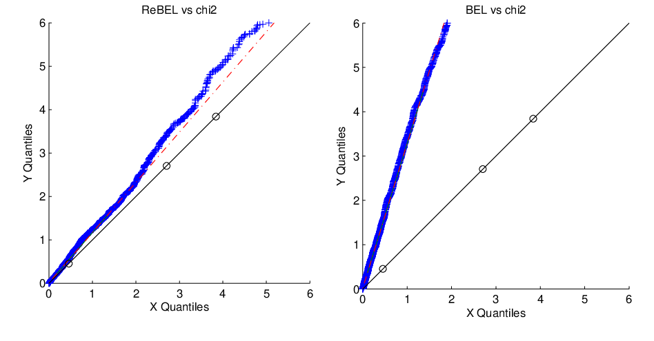
Coverage probabilities at other nominal level can also be investigated, and we make a Monte-Carlo experiment (10 000 repetitions) in order to confirm the adequacy to the asymptotic distribution achieved by the ReBEL algorithm. Data sets length are 10 000.
| Figure 3 should be approximately here |
Figure 3 shows the adequacy of the log likelihood to the asymptotic distribution given by Theorem 4.1. The QQ-plots is almost linear and is close to the 45° line.
6 Conclusion
This paper propose an alternative point of view on dependent data sets and a corresponding semi-parametric methodology. Random length blocks allow to adapt to the dependence structure of the data. We have shown that ReBEL enjoys desirable properties corresponding to that of optimal reference methods for strong-mixing series. Simulations indicate that our algorithm at least competes with Kitamura’s BEL when both methods can be applied.
This method seems to be a promising tool to handle dependent data when classical parametric models do not perform well, for example in presence of asymmetry and non normality of the innovations.
References
- [1] Adamczak, R. (2008), “A tail inequality for suprema of unbounded empirical processes with applications to Markov chains,” Electron. J. Probab., 13, 1000–1034.
- [2] Antoine, B., Bonnal, H., and Renault, E. (2007), “On the efficient use of the informational content of estimating equations: Implied probabilities and Euclidean empirical likelihood,” Journal of Econometrics, 138, 461–487.
- [3] Asmussen, S., Applied Probabilities and Queues, Springer, New York (2003).
- [4] Athreya, K., and Ney, P. (1978), “A new approach to the limit theory of recurrent Markov chains,” Trans. Amer. Math. Soc., 245, 493–501.
- [5] Bertail, P., and Clémençon, S. (2004), “Approximate Regenerative Block-Bootstrap for Markov Chains: second-order properties,” in Compstat 2004 Proceedings, Physica Verlag.
- [6] Bertail, P., and Clémençon, S. (2004), “Edgeworth expansions for suitably normalized sample mean statistics of atomic Markov chains,” Prob. Th. Rel. Fields, 130, 388–414.
- [7] Bertail, P., and Clémençon, S. (2006), “Regeneration-based statistics for Harris recurrent Markov chains,” in Dependence in Probability and Statistics, eds. P. Bertail, P. Doukhan and P. Soulier, Vol. 187 of Lecture Notes in Statistics, Springer.
- [8] Bertail, P., and Clémençon, S. (2006), “Regenerative Block Bootstrap for Markov Chains,” Bernoulli, 12, 689–712.
- [9] Bertail, P., Clémençon, S., and Tressou, J. (2009), “Renewal approach to U-Statistics for Markovian data,” in 41èmes Journées de Statistique, SFdS, Bordeaux, http://hal.archives-ouvertes.fr/inria-00386724/.
- [10] Bertail, P., Gautherat, E., and Harari-Kermadec, H. (2008), “Exponential bounds for multivariate self-normalized sums,” Electronic communication in probability, 13, 628–640.
- [11] Bertail, P., Harari-Kermadec, H., and Ravaille, D. (2007), “-Divergence empirique et vraisemblance empirique généralisée,” Annales d’Économie et de Statistique, pp. 131–157.
- [12] Bolthausen, E. (1982), “The Berry-Esseen Theorem for strongly mixing Harris recurrent Markov Chains,” Z. Wahr. Verw. Gebiete, 60, 283–289.
- [13] Cornec, M., and Harari-Kermadec, H. (2008), “Modeling spot electricity prices with regenerative blocks,” in IASTED ASM.
- [14] Doukhan, P., and Ango Nze, P. (2004), “Weak dependence, models and applications to econometrics,” Econometric Theory, 20, 995–1045.
- [15] Guggenberger, P., and Smith, R.J. (2005), “Generalized empirical likelihood estimators and tests under weak, partial and strong identification,” Econometric Theory, 21, 667–709.
- [16] Götze, F., and Kunsch, H.R. (1996), “Second order correctness of the blockwise bootstrap for stationary observations,” Annals of Statistics, 24, 1914–1933.
- [17] Hall, P., Horowitz, J., and Jing, B.Y. (1995), “On blocking rules for the bootstrap with dependent data,” Biometrika, 82, 561–574.
- [18] Hall, P., and Yao, Q. (2003), “Data tilting for time series,” Journal of the Royal Statistical Society, Series B, 65, 425–442.
- [19] Horowitz, J. (2003), “The Bootstrap in Econometrics,” Statistical Science, 18, 211–218.
- [20] Jain, J., and Jamison, B. (1967), “Contributions to Doeblin’s theory of Markov processes,” Z. Wahrsch. Verw. Geb., 8, 9–40.
- [21] Kallenberg, O., Foundations of modern probability, Springer-Verlag, New York (2002).
- [22] Kitamura, Y. (1997), “Empirical likelihood methods with weakly dependent processes,” Annals of Statistics, 25, 2084–2102.
- [23] Kitamura, Y., “Empirical likelihood methods in Econometrics: theory and practice.” Cowles Foundation discussion paper n°1569. Available at SSRN: http://ssrn.com/abstract=917901 (2006).
- [24] Kitamura, Y., Tripathi, G., and Ahn, H. (2004), “Empirical likelihood-based inference in conditional moment restriction models,” Econometrica, 72, 1667–1714.
- [25] Knight, F. (1975), “A Predictive View of Continuous Time Processes,” Annals of Probability, 3, 573–596.
- [26] Kunsch, H.R. (1989), “The jackknife and the bootstrap for general stationary observations,” Annals of Statistics, 17, 1217–1241.
- [27] Lahiri, S.N., Resampling methods for dependent Data, Springer (2003).
- [28] Li, G., and Wang, Q.H. (2003), “EMPIRICAL LIKELIHOOD REGRESSION ANALYSIS FOR RIGHT CENSORED DATA,” Statistica Sinica, 13, 51–68.
- [29] Lin, L., and Zhang, R. (2001), “Blockwise empirical Euclidean likelihood for weakly dependent processes,” Statistics and Probability Letters, 53, 143–152.
- [30] Meyn, S.P., and Tweedie, R.L., Markov Chains and Stochastic Stability, Cambridge university press (2009).
- [31] Newey, W.K. (1985), “Generalized method of moments specification testing,” Journal of Econometrics, 29, 229–256.
- [32] Newey, W.K., and Smith, R.J. (2004), “Higher Order Properties of GMM and Generalized Empirical Likelihood Estimators,” Econometrica, 72, 219–255.
- [33] Nummelin, E. (1978), “A splitting technique for Harris recurrent chains,” Z. Wahrsch. Verw. Gebiete, 43, 309–318.
- [34] Owen, A.B. (1988), “Empirical Likelihood Ratio Confidence intervals for a Single Functional,” Biometrika, 75, 237–249.
- [35] Owen, A.B. (1990), “Empirical likelihood ratio confidence regions,” Annals of Statistics, 18, 90–120.
- [36] Owen, A.B., Empirical Likelihood, Chapman and Hall/CRC, Boca Raton (2001).
- [37] Qin, Y.S., and Lawless, J. (1994), “Empirical likelihood and General Estimating Equations,” Annals of Statistics, 22, 300–325.
- [38] Rabemananjara, R., and Zakoïan, J.M. (1993), “Threshold Arch Models and Asymmetries in Volatility,” Journal of Applied Econometrics, 8, 31–49.
- [39] Revuz, D., Markov Chains, North-Holland (1984).
- [40] Synowiecki, R. (2007), “Consistency and application of moving block bootstrap for non-stationary time series with periodic and almost periodic structure,” Bernoulli, 13, 1151–1178.
- [41] Teicher, H., and Chow, Y.S., Probability Theory: Independence, Interchangeability, Martingales, Springer-Verlag, New York (1988).
- [42] Tjostheim, D. (1990), “Non-linear time series and Markov chains,” Advances in Applied Probability, 22, 587–611.
- [43] Wang, S., Qian, L., and Carroll, R.J. (2010), “Generalized empirical likelihood methods for analyzing longitudinal data,” Biometrika, 97, 79–93.
Appendix A Proofs
A.1 Lemmas for the atomic case
Denote , and define
To demonstrate Theorem 3.3, we need 2 technical lemmas.
Lemma A.1.
Assume that exists and is full-rank, with ordered eigenvalues . Then, assuming H0 and H0, we have
Therefore, for all with ,
Proof:
The convergence of is a LLN for the sum of a random number of random variables, and is a straightforward corollary of the Theorem 6 of [41, chapter 5.2, page 131].
Lemma A.2.
Assuming H0, H0 and H1, we have
Proof:
By H1,
and then,
By Lemma A.1 of [2], the maximum of i.i.d. real-valued random variables with finite variance is . Let be the maximum of independent copies of , is then such as . As is smaller than , is bounded by and therefore, .
A.2 Proof of Theorem 3.3
The likelihood ratio statistic is the supremum over of . The first order condition at the supremum is then:
| (4) |
Multiplying by and using , we have
Now we may bound the denominators by and then
Multiply both sides by the denominator, or
Dividing by and setting , we have
| (5) |
Now we control the terms between the square brackets. First, by Lemma A.1, is bounded between and . Second, by Lemma A.2, . Third, the CLT applied to the ’s gives . Then, inequality (5) gives
and is then .
A.3 Proof of Theorem 3.6
We keep the notations of the previous subsection. Note that instead of , we have
because . The beginning of the proof is similar to that of Theorem 3.3: the misspecification is not significant at first order: remains . We obtain:
is asymptotically Gaussian with variance , which is the limit in probability of . Therefore,
A.4 Proof of Theorem 3.7
Lemma A.3 (Qin & Lawless, 1994).
Let be i.i.d. observations in and consider a function such that . Suppose that the following hypotheses hold:
- (1)
is positive definite,
- (2)
is continuous and bounded in norm by an integrable function in a neighborhood of ,
- (3)
is bounded by on ,
- (4)
the rank of is ,
- (5)
is continuous and bounded by on .
Then, the maximum empirical likelihood estimator is a consistent estimator and is asymptotically normal with mean zero.
Set
and . Expectation under is then replaced by . Theorem 3.7 is a straightforward application of the Lemma A.3 as soon as the assumptions hold.
By assumption, is of full rank. This implies (1).
By H2(a), there is a neighborhood of and a function such that, for all between and , is continuous on and bounded in norm by . is then continuous as a sum of continuous functions and is bounded for in by . Since is such that , we have by Kac’s Theorem,
The bounding function is then integrable. This gives assumption (2). Assumption (5) is derived from H2(c) by the same arguments.
By H2(d), is bounded by for in , and then
Thus, is also bounded by for in , and hypotheses (3) follows.
By Kac’s Theorem,
which is supposed to be of full rank by H2(b). Thus is of full rank and this gives assumption (4). This concludes the proof of Theorem 3.7.
A.5 Proof of Theorem 4.1
Suppose that we know the real transition density . The chain can then be split with the Nummelin technique as above. We get an atomic chain . Let’s denote by the blocks obtained from this chain. The Theorem (3.3) can then be applied to .
Unfortunately is unknown and then we can not use the . Instead, we have the vectors , built on approximatively regenerative blocks. To prove the Theorem 4.1, we essentially need to control the difference between the two statistics and . This can be done by using Lemmas (5.2) and (5.3) in [8]: under H0, we get
| (6) |
and under H1 and H1,
With some straightforward calculus, we have
| (7) |
Since
equation (6) gives
and
From this and equation (7), we deduce:
| (8) |
Therefore
Using this and the CLT for the , we show that is asymptotically Gaussian.
The same kind of arguments give a control on the difference between empirical variances. Consider
By Lemma (5.3) of [8] we have, under H1 and H1, , and then
| (9) |
The proof of Theorem (3.3) is then also valid for the approximated blocks and reduce to the study of the square of a self-normalized sum based on the pseudo-blocks. We have . Let be the optimum value of , we have
Using the controls given by equations (8) and (9), we get
Developing this product, the main term is and all other terms are , yielding
Results (b), (c) and (d) can be derived from the atomic case by using the same arguments.
| ReBEL | BEL | |
|---|---|---|
| 0.92 | 0.82 | |
| 0.94 | 0.88 | |
| 0.94 | 0.91 |