跳到论文正文
W Papers独立论文阅读器 arXiv:1102.3057 论文正文 计算阅读时间 · 0%
引用这篇论文根据当前论文元数据生成,正式投稿前建议核对。


License: arXiv.org perpetual non-exclusive license
arXiv:1102.3057v2 [cond-mat.other] 30 Jun 2011

Quantum superpositions of a mirror for experimental tests for nonunitary Newtonian gravity

Filippo Maimone, Giovanni Scelza, Adele Naddeo(1), Vinicio Pelino Note: e-mail address: f_maimone@alice.it Note: e-mail address: lucasce73@gmail.com Note: e-mail address: naddeo@sa.infn.it Affiliation: (1)Dipartimento di Fisica “E. R. Caianiello”, Universita`\grave{a} degli Studi di Salerno and CNISM, Unita`\grave{a} di Ricerca di Salerno, Via Ponte don Melillo, 8408484084 Fisciano (SA), Italy
Abstract

Aim of this work is to calculate explicitly the result of the experiment of superposition of a mirror in the Michelson photon cavities interferometric device proposed by Marshall, Simon, Penrose and Bownmeester, as expected within a recently proposed model of non-unitary self-gravity inducing localization. As for other proposals of modifications of Quantum Mechanics in a non-unitary sense, aimed to account for both unitary evolution and irreversible collapse, like in the famous Ghirardi-Rimini-Weber and Pearle’s models, it turns out that, for the experimental parameters proposed, no effect is detectable at all. It is pointed out that the enhancing properties of matter granularity does not substantially change this conclusion. Parameters have also been exploratively varied in a certain range beyond the proposed values. It is shown that within ‘sensible’ parameters, that are not yet attainable within current technology, the model exhibits a peculiar signature with respect to other collapse models as far as parameters space is explored. Besides, the calculation offers a way to see non-unitary gravity at work in a quasi-realistic setting.

Keywords: 
Gravity induced decoherence, spontaneous localization.
pacs
03.65.Ta, 03.65. Yz, 05.40.-a

I Introduction

In the past few decades several proposals of modification of Quantum Mechanics (QM) have appeared in the literature, aimed at unifying its internal fundamental dichotomy between unitary deterministic quantum dynamics and non-linear irreversible state collapse following a measurement process [1]. On the other hand big efforts have been devoted towards an attempt to reconcile Einstein gravity with quantum theory. In this context, some approaches have focused on the possible role of gravity in state function collapse as a result of the incompatibility of general relativity and the unitary time evolution of QM [2, 3, 4, 5]. It has been shown, in fact, that the existence of linear superpositions of states with macroscopic mass-distribution differences would entail a breakdown of classical space-time making the traditional quantum dynamics somehow troubling [2]. As distinct from Penrose proposal, some other detailed collapse models have been proposed, which are based on a spontaneous stochastic state vector reduction: the Ghirardi-Rimini-Weber (GRW) model [6], the quantum mechanics with universal position location model (QMUPL) of wave function collapse [3] and the continuous spontaneous localization (CSL) model [7]. Recently the mechanism of spontaneous symmetry breakdown of time translation symmetry has been invoked as well in order to give rise to the quantum state reduction [8].

In a different proposal, De Filippo introduced a nonunitary model of Newtonian gravity (NNG, from now on), which can be seen as the non-relativistic limit of a classically stable version of higher derivative gravity (see e.g. Ref.[9], references therein). This model presents several appealing features to become a natural candidate for an effective low-energy model of gravity. For example, while reproducing at a macroscopic level the ordinary Newtonian interaction, it presents a mass threshold for gravitational localization, which for ordinary matter densities is around 101110^{11} proton masses [10]. The model can be seen as a realistic version of the nonunitary toy models [11, 12, 13] inspired by the emergence of the information loss paradox [14, 15, 16] from black hole physics. On the other hand the violation of unitarity when matching quantum mechanics and gravity was argued also outside black hole physics, on general consistency grounds [2, 17]. The model affords a mechanism for the evolution of macroscopic coherent superpositions of states into ensembles of pure states, each one of them corresponding – within a future consistent general covariant theory – to an unambiguous space-time. Its features include its ability to produce an evolution of the density matrix compatible with the expectations leading to the phenomenological spontaneous localization models, as it was argued that they should be both nonlinear and nonunitary [5]. While sharing with the other proposals the non-linear non-unitary character, at variance with them, however, it does not present obstructions consistent with its special-relativistic extension [18]. Another success of the model is the emergence of a unified picture for ordinary and black hole entropy as entanglement entropy with hidden degrees of freedom [9], in agreement with Bekenstein-Hawking entropy [19] and Hawking evaporation temperature; that arises from the smoothed singularity of the black hole introduced by the model and paves the way for the quantum foundations of the second law of thermodynamics.

It is important to realize that the subject of a fundamental non-unitarity, and the various detailed mechanisms proposed [2, 17, 20, 3, 4, 21, 22], is not just a matter of philosophy, but could be, in principle, experimentally proved or disproved. Current technological progresses which have being achieved in isolating, manipulating and controlling an higher and higher number of degrees of freedom indicate a not far possibility of detecting fundamental decoherence, which would manifest in a clean way only once the system has been sufficiently protected against the sources of environmental noise [23]. Indeed an experiment designed to detect fundamental deviations from unitary quantum evolution would be of considerable importance. Some technologies and devices have, at present, been recognized to be particularly suitable to create quantum state superpositions which are macroscopically distinct [24]. Among them, there are diffraction of complex molecules up to 2×1032\times 10^{3} proton masses [25], current cat states in SQUID devices [26] and superpositions of atomic matter waves in Bose Einstein condensates [27].

Recent progress in optomechanical systems may soon allow one to make superpositions of even larger objects, such as micro-sized mirrors or cantilevers [28], and to test quantum phenomena at larger scales. In this context an appealing quite recent proposal for the practical realization of the Penrose “gedanken experiment” [2] considers the relatively small CM-displacement of a lump of 101410^{14} proton masses in a interferometric device in which two high-finesse optical cavities are inserted into its arms [29]. The cavity in arm A has a very small end mirror mounted on a micro-mechanical oscillator (cantilever), which suffers the radiation pressure of the photon confined inside it and as a consequence can be excited into a distinguishable quantum state. A single photon incident on a 50-50 beam splitter will realize a superposition of being in either of the two arms; then, the coupling between the photon and the cantilever will lead to an entangled state putting the cantilever into a superposition of distinct positions. After a full mechanical period of the cantilever, it recovers its original position; if the photon leaks out of the cavity at this stage, a revival of the interference (visibility) is observed, provided that the quantum superposition state of the system survives at the intermediate times. Conversely, if the state of the system collapses due to some decoherence mechanism, visibility will not revive. Summarizing, a measurement of the magnitude of the revival of visibility gives a measurement of decoherence occurred in the time interval under consideration.

Our work is devoted to calculate explicitly the output of this experiment [29] according to nonunitary Newtonian gravity model [9, 10, 30, 31]. We would point out that detailed calculations for the expectations of some other collapse models, gravitational or not, have already been done, demonstrating a far reaching possibility to confirm the theory [32, 33, 34].

The plan of the paper is as follows. Section II contains a brief description of the basic NNG model. In Section III we give a qualitative discussion to argue, in the relevant parameter space of the experiment by Marshall et al. [29], the subspaces where gravitational effect could, in principle, be visible with both homogeneous and granular assumption on mirror mass distribution. Section IV is devoted to the application of NNG model to the experiment, and its general solution. Then, in Section V, we use the Wigner function to monitor the mirror’s state, and verify its behavior in time, after a measurement of photons’ state. Finally, in Sec.VI, we draw conclusions and outline perspectives of this work. Calculational details are devoted to Appendices.

II Non-unitary Newtonian Gravity model

The aim of this Section is to briefly recall the key features of the NNG model which we will use for calculations. On the basis of a number of considerations (among which consistency with basic formal relations of QM, approximate energy conservation, classical and quantum behavior of matter, requirement that non-unitary terms have a gravitational origin, etc), it is possible to isolate a two-parameter class of non-unitary gravity models, as discussed in detail in Refs. [9, 10, 30, 31]. We will comment later in the Section on these parameters, while we give here a concise definition of the model in its simplest form, which will allow us to carry out our calculations.

Let H⁡[ψ†,ψ]H[\psi^{\dagger},\psi] be the non-relativistic Hamiltonian of a finite number of particle species, like electrons, nuclei, ions, atoms and/or molecules, where ψ†,ψ\psi^{\dagger},\psi denote the whole set ψj†​(x),ψj​(x)\psi_{j}^{\dagger}(x),\psi_{j}(x) of creation-annihilation operators, i.e. one couple per particle species and spin component. H⁡[ψ†,ψ]H[\psi^{\dagger},\psi] includes the usual electromagnetic interactions accounted for in atomic, molecular and condensed-matter physics. To incorporate that part of gravitational interactions responsible for non-unitarity, one has to introduce complementary creation-annihilation operators ψ~j†​(x),ψ~j​(x)\widetilde{\psi}_{j}^{\dagger}(x),\widetilde{\psi}_{j}(x) and the overall (meta-)Hamiltonian:

Ht​o​t=H⁡[ψ†,ψ]+H⁡[ψ~†,ψ~]+−G∑j,kmjmk∫dxdyψj†​(x)​ψj​(x)​ψ~k†​(y)​ψ~k​(y)|x−y|,\begin{split}H_{tot}&=H[\psi^{\dagger},\psi]+H[\widetilde{\psi}^{\dagger},\widetilde{\psi}]+\\ &-{G}\sum_{j,k}m_{j}m_{k}\int d\textbf{x}d\textbf{y}\frac{\psi_{j}^{\dagger}(\textbf{x})\psi_{j}(\textbf{x})\widetilde{\psi}_{k}^{\dagger}(\textbf{y})\widetilde{\psi}_{k}(\textbf{y})}{|\textbf{x}-\textbf{y}|},\end{split} (II.1)

acting on the product Fψ⊗Fψ~F_{\psi}\otimes F_{\widetilde{\psi}} of Fock spaces of the ψ\psi and ψ~\widetilde{\psi} operators, where mim_{i} is the mass of the ii-th particle species and GG is the gravitational constant. The ψ~\widetilde{\psi} operators obey the same statistics as the corresponding operators ψ\psi, while [ψ,ψ~]−=[ψ,ψ~†]−=0[\psi,\widetilde{\psi}]_{-}=[\psi,\widetilde{\psi}^{\dagger}]_{-}=0.

The meta-particle state space SS is the subspace of Fψ⊗Fψ~F_{\psi}\otimes F_{\widetilde{\psi}}, including the meta-states obtained from the vacuum ||0⟩⟩=|0⟩ψ⊗|0⟩ψ~\left|\left|0\right\rangle\right\rangle=\left|0\right\rangle_{\psi}\otimes\left|0\right\rangle_{\widetilde{\psi}} by applying operators built in terms of the products ψj†​(x)​ψ~j†​(y)\psi_{j}^{\dagger}(x)\widetilde{\psi}_{j}^{\dagger}(y) and symmetrical with respect to the interchange ψ†↔ψ~†\psi^{\dagger}\leftrightarrow\widetilde{\psi}^{\dagger}; as a consequence they have the same number of ψ\psi (physical) and ψ~\widetilde{\psi} (hidden) meta-particles of each species. Since constrained meta-states cannot distinguish between physical and hidden operators, the observable algebra is identified with the physical operator algebra. In view of this, expectation values can be evaluated by preliminarily tracing out the ψ~\widetilde{\psi} operators. In particular, the most general meta-state corresponding to one particle states is represented by

||f⟩⟩=∫dx∫dyf(x,y)ψj†(x)ψ~j†(y)||0⟩⟩.\left|\left|f\right\rangle\right\rangle=\int d\textbf{x}\int d\textbf{y}\,f(\textbf{x},\textbf{y})\psi_{j}^{\dagger}(\textbf{x})\widetilde{\psi}_{j}^{\dagger}(\textbf{y})\left|\left|0\right\rangle\right\rangle. (II.2)
f⁡(x,y)=f⁡(y,x)f(\textbf{x},\textbf{y})=f(\textbf{y},\textbf{x})

This is a consistent definition since Ht​o​tH_{tot} generates a group of (unitary) endomorphisms of SS.

If we prepare a pure nn-particle state, represented in the original setting, excluding gravitational interactions, by

|g⟩=∫dnxg(x1,x2,…,xn)ψj1†(x1)ψj2†(x2)…ψjn†(xn)|0⟩,\left|g\right\rangle=\int d^{n}\textbf{x}\,g\left(\textbf{x}_{1},\textbf{x}_{2},...,\textbf{x}_{n}\right)\psi_{j_{1}}^{\dagger}(\textbf{x}_{1})\psi_{j_{2}}^{\dagger}(\textbf{x}_{2})...\psi_{j_{n}}^{\dagger}(\textbf{x}_{n})\left|0\right\rangle,

its representation in SS is given by the metastate

∫dnxdny(g(x1,…,xn)g(y1,…,yn)×\displaystyle\int d^{n}\textbf{x}\ d^{n}\textbf{y}\biggl(g\left(\textbf{x}_{1},...,\textbf{x}_{n}\right)g\left(\textbf{y}_{1},...,\textbf{y}_{n}\right)\times
×\displaystyle\times ψj1†(x1)…ψjn†(xn)ψ~j1†(y1)…ψ~jn†(yn)||0⟩⟩).\displaystyle\psi_{j_{1}}^{\dagger}(\textbf{x}_{1})...\psi_{j_{n}}^{\dagger}(\textbf{x}_{n})\ \widetilde{\psi}_{j_{1}}^{\dagger}(\textbf{y}_{1})...\widetilde{\psi}_{j_{n}}^{\dagger}(\textbf{y}_{n})\left|\left|0\right\rangle\right\rangle\biggr).

A comment is in order on the possible extensions of the model outlined in Refs.[9, 10, 30, 31]. As said in the beginning of the Section, the phenomenological general model depends on the two parameters (N,ε)(N,\varepsilon). The first refers to the number NN of copies in interaction, which on thermodynamical grounds can be inferred to be 22 (as in the model presented above). It is however interesting to note that the limit N→∞N\rightarrow\infty (with ε=1\varepsilon=1) reproduces the famous non-linear Newton-Schrödinger equation, sometimes considered in the literature as a possible candidate equation for the inclusion of the self-gravity in QM, relevant to the quantum-classical transition [10, 5]. The second, ε,\varepsilon, modulates the degree of nununitarity encoded in the gravitational interaction. The above model definition corresponds to ε=1\varepsilon=1, for which all Newtonian interaction is of nonunitary type. This choice has been made in order to maximize the effect of nonunitarity, while calculating the prediction on the experiment by Marshall et al. [29] in the best model-setting which gives the largest possible deviations from unitarity.

III A semi-quantitative argument for NNG effects in mirror experiment

Before considering the detailed application to the mirror experiment of Ref. [29], in this Section we give a semi-quantitative argument for a gross identification of NNG effects.

When considering self-interaction gravitational energy, the threshold mass of localization, Mt​rM_{tr} ∼1011\sim 10^{11}proton masses (=1.672×10⁻¹⁶​K​g)(=1.672\times 10^{-16}Kg), can be identified in the following way. If M<Mt​rM<M_{tr} the metasystem behaves like an hydrogen-like system, while in the case M>Mt​rM>M_{tr} the hidden mass-copy is quite well superposed to the physical one. As a consequence, the interaction potential can be approximated, within the lowest energy state of the meta-system, by the harmonic oscillator ground state with gaussian wave function width

ΛG=(ℏ(4/3)​π​G​ρs​i​l​M2)1/2,\Lambda_{G}=\left(\frac{\hbar}{\sqrt{\left(4/3\right)\ \pi G\ \rho_{sil}\ M^{2}}}\right)^{1/2},

where ρs​i​l=5×10³\rho_{sil}=5\times 10^{3} K​g/m3Kg/m^{3} is silicon density. For nonunitary gravity to be effective in localizing the mirror, this length scale must be at least comparable with the wave packets separation:

Δ​x=κ​ℏ2​M​ωm,\Delta x=\kappa\sqrt{\frac{\hbar}{2M\omega_{m}}}, (III.1)

where ωm\omega_{m} is the mirror’s frequency and κ\kappa is the optomechanical coupling constant; then the condition Δ​x≳ΛG\Delta x\gtrsim\ \Lambda_{G} amounts to

ϰ≡1ρs​i​l​G​(ωmκ2)2≲1;\varkappa\equiv\ \frac{1}{\rho_{sil}\ G\ }\left(\frac{\omega_{m}}{\kappa^{2}}\right)^{2}\lesssim 1; (III.2)

for the experimental parameters, i.e. ωm≃2​π×500​H​z,ρs​i​l≃5×10³​K​g/m3\omega_{m}\simeq~2\pi\times 500Hz,\ \rho_{sil}\simeq 5\times 10^{3}Kg/m^{3} and κ∼1\ \kappa\sim 1, we get Δ​x≃5.79×10⁻¹⁴​m\Delta x\simeq 5.79\times 10^{-14}m, ϰ∼1013\varkappa\sim 10^{13}. As pointed out in Ref [35], an enhancement in the possibility of observing gravitational decoherence effects is provided by taking into account the real distribution of mass inside a crystal, which is very concentrated within nuclei (see Appendix A.2). In that case, one should consider instead of ρs​i​l\rho_{sil} a matter density ρn​u​c∼104​ρs​i​l\rho_{nuc}\sim 10^{4}\rho_{sil}, given by a silicon nucleus mass divided by its effective radius, which can be estimated as the typical spread of the wavefunction inside a crystal. This leads to ϰ∼109\varkappa\sim 10^{9}, which is still much greater than unity.

It should be stressed that the choice between homogeneous or granular matter distribution is not arbitrary, but is dictated by the experimental situation. As a matter of fact, when the relative displacement of meta-masses Δ​x\Delta x is of the order of the nucleus effective radius, it seems appropriate to take into account granularity; when Δ​x\Delta x is made much greater than interatomic separation then homogeneity assumption appears to be the most suitable one; finally, for Δ​x\Delta x of the order of interatomic separation, if imperfections like dislocations are present in the sample (as it usually happens, even when very accurate preparation methods are used), then meta-masses are likely to ‘feel’ an effective homogeneous masses potential (this is because in the presence of a sufficient number of dislocations, as two meta-nuclei get nearer and nearer in one place, two nuclei in another place in the crystal can equally well go farther and farther from each other); otherwise, for a really perfect crystal granularity should come again into play.

On the other hand, (fundamental) decoherence rate must be at least comparable with (or lower than) a period of natural oscillation of the mirror, which, in its turn, must be comparable with (or lower than) environmental decoherence rate for the experiment to be feasible.

Then the following chain of relations must be satisfied:

EGℏ∼π​κ2​ℏ​G​ρs​i​l​(ρn​u​c)3​ωm∼ωm≳γD,\frac{E_{G}}{\hbar}\sim\frac{\ \pi\kappa^{2}\hbar G\rho_{sil}\left(\rho_{nuc}\right)}{3\omega_{m}}\sim\omega_{m}\gtrsim\gamma_{D}, (III.3)

where EGE_{G} is the gravitational interaction energy of the meta-masses (see Appendix A), γD\gamma_{D} is the environmental decoherence rate of the mirror [29, 32]. With the parameters of the experiment the value ωm=ωmexp≃2​π×500​H​z\omega_{m}=\omega_{m}^{\exp}\simeq 2\pi\times 500Hz has been proposed.

An exploration of parameter space within the exact solution has confirmed that first inequality (III.2) and approximate equality in Eq. (III.3) must hold in order to see some relevant deviation from unitarity.

It should be stressed that, in spite of the improvement of mass size in the mirror experiment with respect to double-slit type experiments, the degree of macroscopicity of superposition is controlled not only by mass but also by space separation of the superposed wave packets.

A comment is in order on the apparent independence of the above result on the mass. The main point is that we have chosen to measure CM state separation in units of coherent states’ size, which means that a larger mass is associated with a smaller unit of length and then, fixing κ\kappa, to a narrower peak separation. One could also choose to fix the absolute separation Δ​x¯\overline{\Delta x}, and express κ≡κ⁡(M,ωm)=Δ​x¯​2​M​ωmℏ\kappa\equiv\kappa\left(M,\omega_{m}\right)=\overline{\Delta x}\sqrt{\frac{2M\omega_{m}}{\hbar}} in the above formulas.

IV Application of NNG model to the mirror experiment

In this Section we carry out interference visibility calculations within the mirror experiment [29] in the framework of the NNG model [9, 10, 30, 31].
To this aim, let us start by defining the gravity-free Hamiltonian

Hf​r​e​e​[b,b†,𝒩A,𝒩B;ωm]=ℏ​ωP​h​(𝒩A+𝒩B)+ℏ​ωm​b†​b−ℏ​g​𝒩A​(b+b†),H_{free}\left[b,b^{\dagger},\mathcal{N}_{A},\mathcal{N}_{B};\omega_{m}\right]=\hbar\omega_{Ph}\left(\mathcal{N}_{A}+\mathcal{N}_{B}\right)+\hbar\omega_{m}b^{\dagger}b-\hbar g\mathcal{N}_{A}\left(b+b^{\dagger}\right),

where g=κ​ωm,g=\kappa\,\omega_{m}, 𝒩A,B\mathcal{N}_{A,B} are the number operators for the photon in the interferometer arms AA and BB respectively, while bb and b†b^{{\dagger}} are the phonon destruction and creation operators associated with the motion of the mirror’s CM. In this way our (meta-)Hamiltonian can be written as

Ht​o​t=Hf​r​e​e​[b,b†,𝒩A;ωm∗]+Hf​r​e​e​[b~,b~†,𝒩~A;ωm∗]−KG​(b+b†)​(b~+b~†),H_{tot}=H_{free}\left[b,b^{\dagger},\mathcal{N}_{A};\omega_{m}^{\ast}\right]+H_{free}\left[\tilde{b},\tilde{b}^{\dagger},\widetilde{\mathcal{N}}_{A};\omega_{m}^{\ast}\right]-K_{G}\left(b+b^{\dagger}\right)(\widetilde{b}+\widetilde{b}^{\dagger}),

with ωm∗=ωm​1+2​KGℏ​ωm\omega_{m}^{\ast}=\omega_{m}\sqrt{1+2\frac{K_{G}}{\hbar\omega_{m}}} (see Appendix A for the calculation of the gravitational interaction strength KGK_{G} in both homogeneous and granular case). In practice, the (relevant degrees of freedom) meta-system is formed by two gravitationally coupled harmonic oscillators and two by two photonic modes, each couple of modes interacting with its own mirror. Then, Schrödinger state at time t is given by:

∥Ψ(t)⟩⟩≡∥Ψ(t)⟩⟩S​c​h=1π2∬d2βd2β~K𝒩A​𝒩~A(β,β~;t)|ψ(t)⟩β⊗|ψ(t)⟩β~,\|\Psi(t)\rangle\rangle\equiv\|\Psi(t)\rangle\rangle_{Sch}=\frac{1}{\pi^{2}}\iint d^{2}\beta d^{2}\widetilde{\beta}\;{\Large K}^{\mathcal{N}_{A}\widetilde{\mathcal{N}}_{A}}(\beta,\widetilde{\beta};t)|\psi(t)\rangle_{\beta}\otimes|\psi(t)\rangle_{\widetilde{\beta}}\,, (IV.1)

where

|ψ(t)⟩β=\displaystyle\left|\psi\left(t\right)\right\rangle_{\beta}=
=\displaystyle= 12e−i​ωP​h​t(|0A1B⟩⊗|βc⟩+f(β)|1A0B⟩⊗|βl⟩),\displaystyle\frac{1}{\sqrt{2}}e^{-i\omega_{Ph}t}\left(\left|0_{A}1_{B}\right\rangle\otimes\left|\beta_{c}\right\rangle+f(\beta)\left|1_{A}0_{B}\right\rangle\otimes\left|\beta_{l}\right\rangle\right),

with

f⁡(β)\displaystyle f(\beta) =\displaystyle= eiκ2(ωm∗t−sinωm∗t)ei​κ​ℑ⁡[β⁡(1−e−i​ωm∗​t)]\displaystyle e^{i\kappa^{2}\left(\omega_{m}^{*}t-\sin\omega_{m}^{*}t\right)}e^{i\kappa\Im\left[\beta\left(1-e^{-i\omega_{m}^{*}t}\right)\right]}
|βc⟩\displaystyle\left|\beta_{c}\right\rangle =\displaystyle= |βe−i​ωm∗​t⟩;|βl⟩=|βe−i​ωm∗​t+κ(1−e−i​ωm∗​t)⟩.\displaystyle\left|\beta e^{-i\omega_{m}^{*}t}\right\rangle;\left|\beta_{l}\right\rangle=\left|\beta e^{-i\omega_{m}^{*}t}+\kappa\left(1-e^{-i\omega_{m}^{*}t}\right)\right\rangle.

Here ℑ⁡(x)\Im{(x)} denotes the imaginary part of xx. Computational details on kernel KK are devoted to Appendix B.

Since the only experimentally accessible quantity is the visibility, defined as twice the off-diagonal term (in the absolute value) of the physical photon’s state ρA​B\rho_{AB}, we are going to calculate this quantity as

V​i​s​(t)=2​|T​rm,m~​T​rP​h~​RV(α)|,Vis\left(t\right)=2\left|Tr_{m,\widetilde{m}}Tr_{\widetilde{Ph}}R_{V}^{\left(\alpha\right)}\right|,

where RV(α)R_{V}^{\left(\alpha\right)} is defined as

RV(α)=⟨1A0B||Ψ⟩⟩⟨⟨Ψ||0A1B⟩.R_{V}^{\left(\alpha\right)}=\left\langle 1_{A}0_{B}\left|\left|\Psi\right\rangle\right\rangle\left\langle\left\langle\Psi\right|\right|0_{A}1_{B}\right\rangle.

It can be shown that visibility has a one-to-one correspondence with von Neumann entropy, which represents a good measure of entanglement for a pure bipartite state [32].

We write the kernel as:

K𝒩A​𝒩~A​(β,β~,t)\displaystyle{\Large K}^{\mathcal{N}_{A}\widetilde{\mathcal{N}}_{A}}(\beta,\widetilde{\beta},t) =\displaystyle= Λ⁡(t)​e−KG2​ℏ2​[4​α​[ℱ1γ∗,Γ++α​ℱ1γ∗,γ∗]+ℱ1Γ+,Γ++ℱ2Γ−,Γ−]​e−|α|2⏟𝕂𝒩A​𝒩~A​(t)×\displaystyle\underset{\mathbb{K}^{\mathcal{N}_{A}\widetilde{\mathcal{N}}_{A}}\left(t\right)}{\underbrace{\Lambda\left(t\right)e^{-\frac{K_{G}}{2\hbar^{2}}\biggl[4\alpha\left[\mathcal{F}_{1}^{\gamma^{\ast},\Gamma_{+}}+\alpha\mathcal{F}_{1}^{\gamma^{\ast},\gamma^{\ast}}\right]+\mathcal{F}_{1}^{\Gamma_{+},\Gamma_{+}}+\mathcal{F}_{2}^{\Gamma_{-},\Gamma_{-}}\biggr]}\;e^{-|\alpha|^{2}}}}\times
×\displaystyle\times e−|β|22−|β~|22+β∗​α+β~∗​α×\displaystyle e^{-\frac{|\beta|^{2}}{2}-\frac{|\widetilde{\beta}|^{2}}{2}+\beta^{*}\alpha+\widetilde{\beta}^{*}\alpha}\times
×\displaystyle\times e−KG2​ℏ2​[(ℱ1γ,γ+ℱ2γ,γ)⏟Fp​β∗2+2​(ℱ1γ,Γ++ℱ2γ,Γ−+2​α​ℱ1γ∗,γ)⏟FΓ​p​β∗]×\displaystyle e^{-\frac{K_{G}}{2\hbar^{2}}\biggl[\underset{F_{p}}{\underbrace{\left(\mathcal{F}_{1}^{\gamma,\gamma}+\mathcal{F}_{2}^{\gamma,\gamma}\right)}}\beta^{\ast 2}+2\underset{F_{\Gamma p}}{\underbrace{(\mathcal{F}_{1}^{\gamma,\Gamma_{+}}+\mathcal{F}_{2}^{\gamma,\Gamma_{-}}+2\alpha\mathcal{F}_{1}^{\gamma^{\ast},\gamma})}}\beta^{\ast}\biggr]}\times
×\displaystyle\times e−KG2​ℏ2​[(ℱ1γ,γ+ℱ2γ,γ)⏟Fp​β~∗2+2​(ℱ1γ,γ−ℱ2γ,γ)⏟Fm​β∗​β~∗+2​(ℱ1γ,Γ+−ℱ2γ,Γ−+2​α​ℱ1γ∗,γ)⏟FΓ​m​β~∗]\displaystyle e^{-\frac{K_{G}}{2\hbar^{2}}\biggl[\underset{F_{p}}{\underbrace{\left(\mathcal{F}_{1}^{\gamma,\gamma}+\mathcal{F}_{2}^{\gamma,\gamma}\right)}}\widetilde{\beta}^{\ast 2}+2\underset{F_{m}}{\underbrace{\left(\mathcal{F}_{1}^{\gamma,\gamma}-\mathcal{F}_{2}^{\gamma,\gamma}\right)}}\beta^{\ast}\widetilde{\beta}^{\ast}+2\underset{F_{\Gamma m}}{\underbrace{(\mathcal{F}_{1}^{\gamma,\Gamma_{+}}-\mathcal{F}_{2}^{\gamma,\Gamma_{-}}+2\alpha\mathcal{F}_{1}^{\gamma^{\ast},\gamma})}}\widetilde{\beta}^{\ast}\biggr]}

where the functions ℱi=ℱi​(ωm∗​t)\mathcal{F}_{i}=\mathcal{F}_{i}(\omega_{m}^{*}t) are defined in Appendix B, Eq. (B.3). Then we proceed to write the products K𝒩A​𝒩~A(β,β~,t)K𝒩A′𝒩~A′∗(β′,β~′,t){\Large K}^{\mathcal{N}_{A}\widetilde{\mathcal{N}}_{A}}(\beta,\widetilde{\beta},t){\Large K}^{\mathcal{N}_{A}^{\prime}\widetilde{\mathcal{N}}_{A}^{\prime}\ast}(\beta^{\prime},\widetilde{\beta}^{\prime},t) in the form (k′=KG/2​ℏ2k^{\prime}=K_{G}/2\hbar^{2}):

𝕂𝒩A​𝒩~A(t)𝕂𝒩A′𝒩~A′∗(t)e−k′​[Fp​β∗2+2​FΓ​p​β∗]⏟K1​(β)e−k′​[Fp​β~∗2+2​Fm​β∗​β~∗+2​FΓ​m​β~∗]⏟K2​(β,β~)e−k′​[Fp∗​β′2+2​FΓ​p∗​β′]⏟K3​(β′)e−k′​[Fp∗​β~′2+2​Fm∗​β′​β~′+2​FΓ​m∗​β~′]⏟K4​(β′,β~′)×\displaystyle\mathbb{K}^{\mathcal{N}_{A}\widetilde{\mathcal{N}}_{A}}\left(t\right)\mathbb{K}^{\mathcal{N}_{A}^{\prime}\widetilde{\mathcal{N}}_{A}^{\prime}\ast}\left(t\right)\underset{{\Large K}_{1}{\Large(\beta)}}{\underbrace{e^{-k^{\prime}\left[F_{p}\beta^{\ast 2}+2F_{\Gamma p}\beta^{\ast}\right]}}}\ \underset{{\LARGE K}_{2}\left(\beta,\widetilde{\beta}\right)}{\underbrace{e^{-k^{\prime}\left[F_{p}\widetilde{\beta}^{\ast 2}+2F_{m}\beta^{\ast}\widetilde{\beta}^{\ast}+2F_{\Gamma m}\widetilde{\beta}^{\ast}\right]}}}\underset{{\LARGE K}_{3}\left(\beta^{\prime}\right)}{\underbrace{e^{-k^{\prime}\left[F^{*}_{p}\beta^{\prime 2}+2F_{\Gamma p}^{*}\beta^{\prime}\right]}}}\ \underset{{\Large K}_{4}\left(\beta^{\prime},\widetilde{\beta}^{\prime}\right)}{\underbrace{e^{-k^{\prime}\left[F^{*}_{p}\widetilde{\beta}^{\prime 2}+2F_{m}^{*}\beta^{\prime}\widetilde{\beta}^{\prime}+2F_{\Gamma m}^{*}\widetilde{\beta}^{\prime}\right]}}}\times
×\displaystyle\times e−|β|22−|β′|22+β∗​α+β′​α∗⏟h⁡(β,β′)​e−|β~|22−|β′~|22+β~∗​α+β~′​α∗⏟g⁡(β~,β~′).\displaystyle\underbrace{e^{-\frac{|\beta|^{2}}{2}-\frac{|\beta^{\prime}|^{2}}{2}+\beta^{*}\alpha+\beta^{\prime}\alpha^{*}}}_{h(\beta,\beta^{\prime})}\underbrace{e^{-\frac{|\widetilde{\beta}|^{2}}{2}-\frac{|\widetilde{\beta^{\prime}}|^{2}}{2}+\widetilde{\beta}^{*}\alpha+\widetilde{\beta}^{\prime}\alpha^{*}}}_{g(\widetilde{\beta},\widetilde{\beta}^{\prime})}.

Let’s calculate the traces:

Trm,m~TrP​h~RV(α)=14​π4eiκ2(ωm∗t−sinω∗mt)×\displaystyle Tr_{m,\widetilde{m}}Tr_{\widetilde{Ph}}R_{V}^{\left(\alpha\right)}=\frac{1}{4\pi^{4}}e^{i\kappa^{2}\left(\omega_{m}^{\ast}t-\sin\omega^{*}_{m}t\right)}\times
×\displaystyle\times ⨌d2(β,β′,β~,β~′)ei​κ​ℑ⁡[β⁡(1−e−i​ωm∗​t)]eβl​βc′⁣∗−12​|βc′|2−12​|βl|2⏟L⁡(β,β′)[K10(β,β~)K00∗(β′,β~′)eβ~c​β~c′⁣∗−12​|β~c|2−12​|β~c′|2⏟Hc​(β~,β~′)+\displaystyle\iiiint d^{2}(\beta,\beta^{\prime},\widetilde{\beta},\widetilde{\beta}^{\prime})\;e^{i\kappa\Im[\beta(1-e^{-i\omega_{m}^{*}t})]}\underset{{\Large L}\left(\beta,\beta^{\prime}\right)}{\underbrace{e^{\beta_{l}\beta_{c}^{\prime\ast}-\frac{1}{2}\left|\beta^{\prime}_{c}\right|^{2}-\frac{1}{2}\left|\beta_{l}\right|^{2}}}}\biggl[{\Large K}^{10}(\beta,\widetilde{\beta}){\Large K}^{00\ast}(\beta^{\prime},\widetilde{\beta}^{\prime})\underset{{\Large H}_{c}\left(\widetilde{\beta},\widetilde{\beta}^{\prime}\right)}{\underbrace{e^{\widetilde{\beta}_{c}\widetilde{\beta}_{c}^{\prime\ast}-\frac{1}{2}\left|\widetilde{\beta}_{c}\right|^{2}-\frac{1}{2}\left|\widetilde{\beta}_{c}^{\prime}\right|^{2}}}}\;+
+\displaystyle+ K11(β,β~)K01∗(β′,β~′)ei​κ​ℑ⁡[β~​(1−e−i​ωm∗​t)]⏟ε⁡(β~)e−i​κ​ℑ⁡[β~′​(1−e−i​ωm∗​t)]⏟δ⁡(β~′)eβ~l​β~l′⁣∗−12​|β~l|2−12​|β~l′|2⏟Hl​(β~,β~′)].\displaystyle{\Large K}^{11}(\beta,\widetilde{\beta}){\Large K}^{01\ast}(\beta^{\prime},\widetilde{\beta}^{\prime})\underbrace{e^{i\kappa\Im[\widetilde{\beta}(1-e^{-i\omega_{m}^{*}t})]}}_{\varepsilon(\widetilde{\beta})}\underbrace{e^{-i\kappa\Im[\widetilde{\beta}^{\prime}(1-e^{-i\omega_{m}^{*}t})]}}_{\delta(\widetilde{\beta}^{\prime})}\underset{{\Large H}_{l}\left(\widetilde{\beta},\widetilde{\beta}^{\prime}\right)}{\underbrace{e^{\widetilde{\beta}_{l}\widetilde{\beta}_{l}^{\prime\ast}-\frac{1}{2}\left|\widetilde{\beta}_{l}\right|^{2}-\frac{1}{2}\left|\widetilde{\beta}_{l}^{\prime}\right|^{2}}}}\biggr].

Visibility is then given by two contributions:

V​i​s​(t)=2​|T​rm,m~​T​rP​h~​RV(α)|=2​|(I)+(I​I)|.Vis\left(t\right)=2\left|Tr_{m,\widetilde{m}}Tr_{\widetilde{Ph}}R_{V}^{\left(\alpha\right)}\right|=2\left|\left(I\right)+\left(II\right)\right|. (IV.2)

Here we do not write the explicit integrals for (I)(I) and (I​I)(II), which can be found in Appendix C; it is worth noting that, if we discard their photons number dependence, they are formally similar. In the free case of no NNG interaction, i.e. by putting k′=0k^{\prime}=0, and for α=0\alpha=0, we get

(I)≡(I​I)\displaystyle(I)\equiv(II) =\displaystyle= 14|Λ(t)|2eiκ2(ωmt−sinωmt)e−κ2(1−cosωmt)(for k′=0, ωm∗=ωm and |Λ(t)|2=1)\displaystyle\frac{1}{4}|\Lambda(t)|^{2}e^{i\kappa^{2}\left(\omega_{m}t-\sin\omega_{m}t\right)}\,e^{-\kappa^{2}(1-\cos\omega_{m}t)}\qquad\bigl(\mbox{for }k^{\prime}=0,\mbox{ }\omega_{m}^{*}=\omega_{m}\mbox{ and }|\Lambda(t)|^{2}=1\bigr)

as found in [29].

Refer to caption
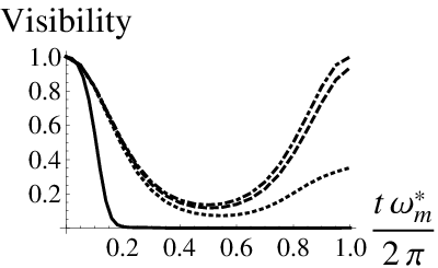
Figure 1: Interference visibility as a function of time in the homogeneous case plotted for κ=1,\kappa=1, m​a​s​s=5×10⁻¹²​k​gmass=5\times 10^{-12}kg for the mirror size L=10−5​mL=10^{-5}m and several values of the frequency: ωm=ωme​x​p×10−5\omega_{m}=\omega_{m}^{exp}\times 10^{-5} (dot-dashed), ωm=ωme​x​p×10−6\omega_{m}=\omega_{m}^{exp}\times 10^{-6} dashed, ωm=5​ωme​x​p×10−7\omega_{m}=5\,\omega_{m}^{exp}\times 10^{-7} (dotted) and ωm=ωme​x​p×10−7\omega_{m}=\omega_{m}^{exp}\times 10^{-7} (continuous black line). Visibility and time are expressed in dimensionless units.

The behavior of visibility for κ=1\kappa=1 and four different values of ωm\omega_{m} is depicted in Figure 1. The first case shows no difference with the free case, and the remaining three, in decreasing order, progressively give a more and more reduction of revival effect at the end of the cycle. A direct comparison can be made with the predictions of other phenomenological collapse models, like GRW, QMUPL and CLS [5, 33]. Let us focus, for example, on the GRW model [6]. In such a case the explicit formula for visibility is

V​i​s​(t)=V​i​s0​(t)​e−3​κ2​ℏ​η02​μn​u​c​ωm​(t−43​sinωmtωm+sin⁡2​ωm​t6​ωm),Vis\left(t\right)=Vis_{0}\left(t\right)\ e^{-\frac{3\ \kappa^{2}\hbar\ \eta_{0}}{2\ \mu_{nuc}\,\omega_{m}}\left(t-\frac{4}{3}\frac{\sin\omega_{m}t}{\omega_{m}}+\frac{\sin 2\omega_{m}t}{6\,\omega_{m}}\right)},

where V​i​s0Vis_{0} is the visibility in the free case, i.e. in the absence of any mechanism of decoherence (of fundamental or environmental nature), η0≃0.5×10⁻²​s−1​m−2\eta_{0}\simeq 0.5\times 10^{-2}s^{-1}m^{-2} and μn​u​c∼1.67×10⁻²⁷​k​g\mu_{nuc}\sim 1.67\times 10^{-27}kg is nucleon mass. Notice that also in this case no explicit dependence on mass appears. It turns out that in the “worst” NNG case (ωm=ωmexp×10−7\omega_{m}=\omega_{m}^{\exp}\times 10^{-7}), in which visibility goes practically to zero, GRW predicts a visibility lowering at the end of the cycle of about 0.5%0.5\% with respect to the free case. It is interesting to note that for smaller Δ​x\Delta x an enhancement of the effect’s observability comes from the consideration of granularity. As discussed in the previous Section, in fact, for Δ​x∼10−12\Delta x\sim 10^{-12} or less matter granularity may come into play; as a consequence, we obtain that already for ωm=ωmexp×10−3\omega_{m}=\omega_{m}^{\exp}\times 10^{-3} visibility behaves in a similar way to the homogeneous case with ωm=ωmexp×10−6\omega_{m}=\omega_{m}^{\exp}\times 10^{-6} (dashed curve of Figure 1).

V Monitoring the mirror’s state: the Wigner function

In the previous Section we have considered a measure of photons’ interference, and shown that with a proper choice of parameters one gets a reduced revival effect at the end of one oscillation period. Here we want to elucidate about the mirror’s state soon after a photon measurement process. For monitoring mirror’s state, and to get a physical insight of what’s going on, we use the Wigner function. As it is well known, this quasi-distribution have both positive and negative parts, the latter being a signature of quantum coherence survival. It is expected that the action of NNG-induced decoherence would reduce, after some time, the interference patterns in the Wigner distribution.

We calculate the Wigner function starting from the expression:

W⁡(x,p,t)=12​ℏ​π2​∫d2​λ​e−λ​η∗+λ∗​η​T​r​[ρm​(t)​eλ​b^†−λ∗​b^],W\left(x,p;t\right)=\frac{1}{2\hbar\pi^{2}}\int d^{2}\lambda\ e^{-\lambda\eta^{\ast}+\lambda^{\ast}\eta}\ Tr\left[\rho_{m}\left(t\right)\ e^{\lambda\widehat{b}^{\dagger}-\lambda^{\ast}\widehat{b}}\right], (V.1)

with

η=i​p2​M​ωm∗​ℏ+x​M​ωm∗2​ℏ,\eta=\frac{ip}{\sqrt{2M\omega_{m}^{\ast}\hbar}}+x\sqrt{\frac{M\omega_{m}^{\ast}}{2\hbar}},

where ρm\rho_{m} is the reduced density matrix of the mirror after a photon detection [36]. Following [32], we take this measurement as the process projecting (physical) photons’ state onto the state

|φ⟩=12(|0A,1B⟩+ei​θ|1A,0B⟩),|\varphi\rangle=\frac{1}{\sqrt{2}}\left(|0_{A},1_{B}\rangle+e^{i\theta}|1_{A},0_{B}\rangle\right),

where θ\theta is a phase constant (it can be shown that the corresponding results are quasi-independent of θ\theta and then we put θ=0\theta=0). Correspondingly, mirror’s density matrix is (||φ⟩⟩≡|φ⟩⊗|φ~⟩\left|\left|\varphi\right\rangle\right\rangle\equiv\left|\varphi\right\rangle\otimes\left|\widetilde{\varphi}\right\rangle)

ρm(t)=TrP​h,P​h~,m~[(||φ⟩⟩⟨⟨φ||⊗1)||Ψ(t)⟩⟩⟨⟨Ψ(t)||].\rho_{m}\left(t\right)=Tr_{Ph,\widetilde{Ph},\widetilde{m}}\left[\left(\left|\left|\varphi\right\rangle\right\rangle\left\langle\left\langle\varphi\right|\right|\otimes{\large 1}\right)~\left|\left|\Psi\left(t\right)\right\rangle\right\rangle\left\langle\left\langle\Psi\left(t\right)\right|\right|\right].

After some calculations, we get the Wigner function as

W⁡(x,p,t)\displaystyle W\left(x,p;t\right) =\displaystyle= 12​ℏ​π2​∫d2​λ​[e−λ​η∗+λ∗​η​T​r​[ρm​(t)​eλ​b†−λ∗​b]]=\displaystyle\frac{1}{2\hbar\pi^{2}}\int d^{2}\lambda\ \left[e^{-\lambda\eta^{\ast}+\lambda^{\ast}\eta}\ Tr\left[\rho_{m}\left(t\right)\ e^{\lambda b^{\dagger}-\lambda^{\ast}b}\right]\right]= (V.2)
=\displaystyle= 14​ℏ​π5∫d2(β,β~,β′,β′~)e−2​η​η∗[α1e−βcβc′∗−12|βc|2−12|βc′|2+2βcη∗+2βc′∗η+α2e−βlβl′∗−12|βl|2−12|βl′|2+2βlη∗+2βl′∗η\displaystyle\frac{1}{4\hbar\pi^{5}}\int d^{2}(\beta,\widetilde{\beta},\beta^{\prime},\widetilde{\beta^{\prime}})e^{-2\eta\eta^{\ast}}\biggl[\alpha_{1}e^{-\beta_{c}\beta_{c}^{\prime^{\ast}}-\frac{1}{2}\left|\beta_{c}\right|^{2}-\frac{1}{2}\left|\beta_{c}^{\prime}\right|^{2}+2\beta_{c}\eta^{\ast}+2\beta_{c}^{\prime^{\ast}}\eta}+\alpha_{2}e^{-\beta_{l}\beta_{l}^{\prime^{\ast}}-\frac{1}{2}\left|\beta_{l}\right|^{2}-\frac{1}{2}\left|\beta_{l}^{\prime}\right|^{2}+2\beta_{l}\eta^{\ast}+2\beta_{l}^{\prime^{\ast}}\eta}
+\displaystyle+ α3e−βcβl′∗−12|βc|2−12|βl′|2+2βcη∗+2βl′∗η+α4e−βlβc′∗−12|βl|2−12|βc′|2+2βlη∗+2βc′∗η].\displaystyle\alpha_{3}e^{-\beta_{c}\beta_{l}^{\prime^{\ast}}-\frac{1}{2}\left|\beta_{c}\right|^{2}-\frac{1}{2}\left|\beta_{l}^{\prime}\right|^{2}+2\beta_{c}\eta^{\ast}+2\beta_{l}^{\prime^{\ast}}\eta}+\alpha_{4}e^{-\beta_{l}\beta_{c}^{\prime^{\ast}}-\frac{1}{2}\left|\beta_{l}\right|^{2}-\frac{1}{2}\left|\beta_{c}^{\prime}\right|^{2}+2\beta_{l}\eta^{\ast}+2\beta_{c}^{\prime^{\ast}}\eta}\biggr].

Explicit expressions for α1,α2,α3\alpha_{1},\alpha_{2},\alpha_{3} and α4\alpha_{4}, together with calculational details, are reported in Appendix D.

Results for κ=2\kappa=2 and ωm=ωmexp×10−5\omega_{m}=\omega_{m}^{\exp}\times 10^{-5} and ωm=5​ωmexp×10−7\omega_{m}=~5\,\omega_{m}^{\exp}\times 10^{-7}, are shown in Figures 2 and 3 respectively for the homogeneous case. As seen for visibility, in the case of (proposed) experimental values, Wigner function after measurement is undistinguishable from the free case. For the second (presently unattainable) much smaller value of ωm\omega_{m}, after a certain time a diminution of interference fringes is observed together with a contextual lowering of the first rest peak.

Refer to caption
Refer to caption
Refer to caption
Refer to caption
Refer to caption
Figure 2: (Color online) Wigner function in the homogeneous case for κ=2,\kappa=~2, ωm=ωme​x​p×10−5,\omega_{m}=\omega_{m}^{exp}\times 10^{-5}, for the mirror size L=10−5​mL=10^{-5}m and for different intermediate times in a complete mirror oscillation. The variables xx and pp are in the ranges {−10​δ​x,10​δ​x}\{-10\delta x,10\delta x\} and {−10​δ​p,10​δ​p}\{-10\delta p,10\delta p\} with δ​x≐ℏ2​M​ωm∗\delta x\doteq\sqrt{\frac{\hbar}{2M\omega_{m}^{*}}} and δ​p≐ℏ​M​ωm∗2\delta p\doteq\sqrt{\frac{\hbar M\omega_{m}^{*}}{2}}, while τ=ωm∗​t\tau=\omega_{m}^{*}t. In the case with ωm=ωme​x​p,\omega_{m}=\omega_{m}^{exp}, as in the absence of gravity, we get qualitatively the same graphics. All quantities are expressed in dimensionless units.
Refer to caption
Refer to caption
Refer to caption
Refer to caption
Refer to caption
Figure 3: (Color online) Wigner function for ωm=5​ωme​x​p×10−7\omega_{m}=~5\,\omega_{m}^{exp}\times 10^{-7}. All the other parameters are as above. All quantities are expressed in dimensionless units.

VI Conclusions and perspectives

In this paper the output of the mirror experiment proposed by Marshall et al. [29] has been calculated within the framework of NNG, assuming both homogeneous and granular mass distributions. By varying the experimental parameters in a wide range beyond the proposed values [29], a window of “sensible” parameters has been found in which the NNG induced decoherence effect is manifest.

In conclusion, even if the experimental test of nonunitary gravity has been proved to lie beyond current technology yet, requiring an unprecedented control of decoherence, its peculiar form of self-gravitational interaction has been shown to be in principle distinguishable from the action of other collapse models. An exploration of the relevant parameter space could in fact, in a feasible experiment, lead to a clear distinction of the most appropriate model. The signature of NNG model is ultimately connected with the fact that fundamental interaction occurs with a “simple” system (the mirror’s copy in this case) rather than with a fundamental “thermal bath” random field leading to a visibility output somehow indistinguishable from the effect of temperature. This is essentially due to the laboratory artificially created superposition state, while in naturally occurring circumstances it is expected that “fundamental environment”, being as complex as the system itself, could eventually lead to auto-thermalization effects.
In spite of the huge technical challenges, however, we believe that due to the rapid progress in developing high-quality micro-optomechanical devices, a prototypal experiment of this type could be soon realized.

A remark is finally in order concerning a finite temperature inclusion into the model. It should be clear that, when our initial knowledge of the system state is characterized by a density matrix like a thermal state, there is no unique prescription to associate it with a pure meta-state. In such a case one has to consider the possibility of using mixed meta-states to encode our incomplete knowledge. This more general case, independently of the specific experiment treated here, will pave the way towards a generalized model of gravity induced thermalization. Such an interesting issue will be addressed in a future publication [37].

Acknowledgements

The authors would like to thank Mario Salerno for discussions and useful comments on the manuscript. Anonymous referee’s critical comment, pointing out an important issue of the work, is also kindly acknowledged.

Appendix A Interacting gravitational potential of the meta-mirrors

In this Appendix the gravitational interaction potential between meta-mirrors is computed within the two assumption of homogeneous and granular mass distributions.

A.1 The case with homogeneous masses

Let’s consider the Newtonian potential energy for two particles with masses M1M_{1} and M2M_{2}

V⁡(r12)=−G​M1​M2r12.V\left(r_{12}\right)=-G\frac{M_{1}M_{2}}{r_{12}}.

Starting from the initial condition where the two mirrors of length LL are overlapped, we consider the shifting of the first mirror of d/2d/2 along z1z_{1} positive axis and the second one along z2z_{2} negative axis. Because of the very small relative displacement dd between the meta-mirrors (which is at maximum of the order of the size of the wave-function describing, in the ordinary setting, the CM coordinate of the mirror), it is enough to calculate the quadratic term of the expansion in the distance of the total gravitational interaction energy

V⁡(d)\displaystyle V\left(d\right) =\displaystyle= ∫−(L+d)/2(L−d)/2dz1∫−(L−d)/2(L+d)/2dz2𝒱(z1,z2)\displaystyle\int_{-\left(L+d\right)/2}^{\left(L-d\right)/2}dz_{1}\int_{-(L-d)/2}^{\left(L+d\right)/2}dz_{2}\;\mathcal{V}\left(z_{1},z_{2}\right)
=\displaystyle= (∫−L/2L/2dz1+∫−(L+d)/2−L/2dz1−∫(L−d)/2L/2dz1)(∫−L/2L/2dz2−∫−L/2−(L−d)/2dz2+∫L/2(L+d)/2dz2)𝒱(z1,z2)\displaystyle\left(\int_{-L/2}^{L/2}dz_{1}+\int_{-(L+d)/2}^{-L/2}dz_{1}-\int_{\left(L-d\right)/2}^{L/2}dz_{1}\right)\left(\int_{-L/2}^{L/2}dz_{2}-\int_{-L/2}^{-\left(L-d\right)/2}dz_{2}+\int_{L/2}^{\left(L+d\right)/2}dz_{2}\right)\mathcal{V}\left(z_{1},z_{2}\right)
=\displaystyle= Const.+12​[𝒱⁡(L2,−L2)−𝒱⁡(L2,L2)]​d2+O⁡(d3),\displaystyle\mbox{{Const.}}+\frac{1}{2}\left[\mathcal{V}\left(\frac{L}{2},-\frac{L}{2}\right)-\mathcal{V}\left(\frac{L}{2},\frac{L}{2}\right)\right]d^{2}+O\left(d^{3}\right),

where 𝒱⁡(z1,z2)​δ​z1​δ​z2\mathcal{V}\left(z_{1},z_{2}\right)\delta z_{1}\delta z_{2} is the interaction energy of two square infinitesimally tiny mirror sheets parallel to the x−yx-y plane,

𝒱⁡(z1,z2)=∬−L2L2d​x1​d​y1​∬−L2L2d​x2​d​y2​(−G​ρ2r12).\mathcal{V}\left(z_{1},z_{2}\right)=\iint\limits_{-\frac{L}{2}}^{\frac{L}{2}}d\,x_{1}d\,y_{1}\iint\limits_{-\frac{L}{2}}^{\frac{L}{2}}d\,x_{2}d\,y_{2}\left(-\frac{G\,\rho^{2}}{r_{12}}\right).

Here we have used the assumption that, for example, ∫−(L+d)/2−L/2dz1∫−L/2L/2dz2𝒱(z1,z2)=d2∫−L/2L/2𝒱(−L2,z2)dz2.\int_{-(L+d)/2}^{-L/2}dz_{1}\int_{-L/2}^{L/2}dz_{2}\mathcal{V}(z_{1},z_{2})=~\frac{d}{2}\int_{-L/2}^{L/2}\mathcal{V}(-\frac{L}{2},z_{2})dz_{2}. In this way the terms linear in dd vanish. Defining the non-dimensional coordinates x1′=x1/L,y1′=y1/L,x_{1}^{\prime}=x_{1}/L,\ y_{1}^{\prime}=y_{1}/L,\ and so on, we get:

[𝒱⁡(L2,−L2)−𝒱⁡(L2,L2)]=\displaystyle\left[\mathcal{V}\left(\frac{L}{2},-\frac{L}{2}\right)-\mathcal{V}\left(\frac{L}{2},\frac{L}{2}\right)\right]=
=\displaystyle= G​M2L3∬−1/21/2dx1′dy1′∬−1/21/2dx2′dy2′(1[(x1′−x2′)2+(y1′−y2′)2]1/2−1[(x1′−x2′)2+(y1′−y2′)2+1]1/2)=\displaystyle\frac{G\,M^{2}}{L^{3}}\iint\limits_{-1/2}^{1/2}dx_{1}^{\prime}dy_{1}^{\prime}\iint\limits_{-1/2}^{1/2}dx_{2}^{\prime}dy_{2}^{\prime}\left(\frac{1}{\left[\left(x_{1}^{\prime}-x_{2}^{\prime}\right)^{2}+\left(y_{1}^{\prime}-y_{2}^{\prime}\right)^{2}\right]^{1/2}}-\frac{1}{\left[\left(x_{1}^{\prime}-x_{2}^{\prime}\right)^{2}+\left(y_{1}^{\prime}-y_{2}^{\prime}\right)^{2}+1\right]^{1/2}}\right)=
=\displaystyle= 4​G​M2L3​∫01d​ξ−​∫01−ξ−d​ξ+​∫01d​η−​∫01−η−d​η+​(1[ξ−2+η−2]1/2−1[ξ−2+η−2+1]1/2)\displaystyle 4\frac{G\,M^{2}}{L^{3}}\int_{0}^{1}d\xi_{-}\int_{0}^{1-\xi_{-}}d\xi_{+}\int_{0}^{1}d\eta_{-}\int_{0}^{1-\eta_{-}}d\eta_{+}\left(\frac{1}{\left[\xi_{-}^{2}+\eta_{-}^{2}\right]^{1/2}}-\frac{1}{\left[\xi_{-}^{2}+\eta_{-}^{2}+1\right]^{1/2}}\right)
=\displaystyle= 4​G​M2L3​∫01d​ξ−​∫01d​η−​(1−ξ−)​(1−η−)​(1[ξ−2+η−2]1/2−1[ξ−2+η−2+1]1/2)=2​π3​G​M2L3,\displaystyle 4\frac{G\,M^{2}}{L^{3}}\int_{0}^{1}d\xi_{-}\int_{0}^{1}d\eta_{-}\left(1-\xi_{-}\right)\left(1-\eta_{-}\right)\left(\frac{1}{\left[\xi_{-}^{2}+\eta_{-}^{2}\right]^{1/2}}-\frac{1}{\left[\xi_{-}^{2}+\eta_{-}^{2}+1\right]^{1/2}}\right)=\frac{2\pi}{3}\frac{G\,M^{2}}{L^{3}},

where we have introduced the new variables ξ±=x1′±x2′\xi_{\pm}=x_{1}^{\prime}\pm x_{2}^{\prime} and η±=y1′±y2′\eta_{\pm}=y_{1}^{\prime}\pm y_{2}^{\prime}.

Then we obtain

V⁡(d)=C​o​n​s​t.+π3​G​M​ρs​i​l​d2,V\left(d\right)=Const.+\frac{\pi}{3}GM\,\rho_{sil}\;d^{2},

from which, writing the interaction term in the meta-Hamiltonian as −KG​(b+b†)​(b~+b~†)-K_{G}\left(b+b^{\dagger}\right)(\widetilde{b}+\widetilde{b}^{\dagger}), we get

KGhom=π​ℏ​G​ρs​i​l3​ωm.K_{G}^{\hom}=\frac{\pi\hbar G\rho_{sil}}{3\omega_{m}}.

A.2 The case with matter-granularity effect

Looking at the meta-mirrors as aggregates of atoms disposed in a lattice {Rj}\{\textbf{R}_{j}\}, we are led to consider the gravitational potential between the meta-crystals described by the state (to be symmetrized)

|𝚽C​r​y​s​t​a​l(−d/2)⟩⊗|𝚽~C​r​y​s​t​a​l(+d/2)⟩,\left|\mathbf{\Phi}_{Crystal}^{\left(-d/2\right)}\right\rangle\otimes\left|\widetilde{\mathbf{\Phi}}_{Crystal}^{\left(+d/2\right)}\right\rangle,

where superscripts parameters ∓d/2\mp d/2 refer to the center of mass displacements from the origin of coordinate system along, say, x−x-axis. The problem is similar to that of potential between two atoms or molecules, where (within the Born-Oppenheimer approximation) nuclei positions are treated as parameters of the atoms/molecules.
The interaction potential is then given by (𝐝≡(d,0,0)\mathbf{d}\equiv\left(d,0,0\right))

V⁡(d)=−Gmn​u​c2∫∫d𝐱d𝐲⟨𝚽C​r​y​s​t​a​l(−d/2)|ψ†(𝐱)ψ(𝐱)|𝚽C​r​y​s​t​a​l(−d/2)⟩⟨𝚽~C​r​y​s​t​a​l(+d/2)|ψ~†(𝐲)ψ~(𝐲)|𝚽~C​r​y​s​t​a​l(+d/2)⟩|𝐱−𝐲|=−Gmn​u​c2(mn​u​c​ωC​r​y​s​t​a​lℏ​π)∑h,k=1Nn​u​c∫∫d𝐱d𝐲e−mn​u​c​ωC​r​y​s​t​a​lℏ[(𝐱−𝐑h(−d/2))2+(𝐲−𝐑k(+d/2))2]|𝐱−𝐲|≃−Gmn​u​c2(mn​u​c​ωC​r​y​s​t​a​lℏ​π)Nn​u​c∫∫d𝐱d𝐲e−mn​u​c​ωC​r​y​s​t​a​lℏ​[(𝐱+𝐝/2)2+(𝐲−𝐝/2)2]|𝐱−𝐲|,\displaystyle\begin{split}V\left(d\right)&=-Gm_{nuc}^{2}\int\int d\mathbf{x}d\mathbf{y}\frac{\left\langle\mathbf{\Phi}_{Crystal}^{\left(-d/2\right)}\right|\psi^{\dagger}\left(\mathbf{x}\right)\psi\left(\mathbf{x}\right)\left|\mathbf{\Phi}_{Crystal}^{\left(-d/2\right)}\right\rangle\left\langle\widetilde{\mathbf{\Phi}}_{Crystal}^{\left(+d/2\right)}\right|\widetilde{\psi}^{\dagger}\left(\mathbf{y}\right)\widetilde{\psi}\left(\mathbf{y}\right)\left|\widetilde{\mathbf{\Phi}}_{Crystal}^{\left(+d/2\right)}\right\rangle}{\left|\mathbf{x}-\mathbf{y}\right|}\\ &=-Gm_{nuc}^{2}\left(\frac{m_{nuc}\omega_{Crystal}}{\hbar\pi}\right)\sum_{h,k=1}^{N_{nuc}}\int\int d\mathbf{x}d\mathbf{y}\frac{e^{-\frac{m_{nuc}\omega_{Crystal}}{\hbar}\left[\left(\mathbf{x}-\mathbf{R}_{h}^{(-d/2)}\right)^{2}+\left(\mathbf{y}-\mathbf{R}_{k}^{(+d/2)}\right)^{2}\right]}}{\left|\mathbf{x}-\mathbf{y}\right|}\\ &\simeq-Gm_{nuc}^{2}\left(\frac{m_{nuc}\omega_{Crystal}}{\hbar\pi}\right)N_{nuc}\int\int d\mathbf{x}d\mathbf{y}\frac{e^{-\frac{m_{nuc}\omega_{Crystal}}{\hbar}\left[\left(\mathbf{x}+\mathbf{d}/2\right)^{2}+\left(\mathbf{y}-\mathbf{d}/2\right)^{2}\right]}}{\left|\mathbf{x-y}\right|},\end{split} (A.1)

where, for simplicity, Einstein model for the crystal has been used, with ωC​r​y​s​t​a​l≡\omega_{Crystal}\equiv Einstein frequency ≃10​T​H​z\simeq 10\,THz, mn​u​c≃4.7×10⁻²⁶​K​gm_{nuc}\simeq 4.7\times 10^{-26}Kg is nucleus mass, Nn​u​c≃1014N_{nuc}\simeq 10^{14} the number of nuclei. In the last line of the above formula, we have made the assumption that the nuclei wavefunction spreads are much lower than interatomic distance, and that the formers are greater than dd. To get a simple estimate, we can consider the interaction between interpenetrating spheres of radius ℏ2​mn​u​c​ωC​r​y​s​t​a​l\sqrt{\frac{\hbar}{2m_{nuc}\omega_{Crystal}}} separated by a distance dd, so that

V⁡(d)≃C​o​n​s​t.+23​G​M​ρn​u​c​d2,V\left(d\right)\simeq Const.+\frac{2}{3}GM\rho_{nuc}\;d^{2},

giving the (enhanced) gravitational coupling

KG gran=2​ℏ​G​ρn​u​c3​ωm≃104×KGhom.K_{G}^{\text{ gran}}=\frac{2\hbar G\rho_{nuc}}{3\omega_{m}}\simeq 10^{4}\times K_{G}^{\text{hom}}.

Appendix B Dynamical evolution of the meta-system

In the following we study in detail the dynamical evolution of the meta-system. As initial meta-state we take

||Ψ(0)⟩⟩=12[(|0A1B⟩+|1A0B⟩)|α⟩]⊗[(|0A~1B~⟩+|1A~0B~⟩)|α~⟩]≡|ψ(0)⟩⊗|ψ(0)⟩\left|\left|\Psi\left(0\right)\right\rangle\right\rangle=\frac{1}{2}\left[\left(\left|0_{A}1_{B}\right\rangle+\left|1_{A}0_{B}\right\rangle\right)\ \left|\alpha\right\rangle\right]\otimes\left[\left(\left|0_{\tilde{A}}1_{\tilde{B}}\right\rangle+\left|1_{\tilde{A}}0_{\tilde{B}}\right\rangle\right)\ \left|\widetilde{\alpha}\right\rangle\right]\equiv\left|\psi\left(0\right)\right\rangle\otimes\left|\psi\left(0\right)\right\rangle (B.1)

where general coherent states α1\alpha_{1} and α2\alpha_{2} are considered, although acceptable meta-states must be symmetrized with respect to the physical and hidden parts.

Let’s start by calculating the meta-state at time tt. We will use the interaction picture, defining

||Ψ(t)⟩⟩I​n​t=ei⁡(Hf​r​e​e​[b,b†,𝒩A,𝒩B;ωm∗]+Hf​r​e​e​[b~,b~†,𝒩A∼,𝒩B∼;ωm∗])​t/ℏ||Ψ(t)⟩⟩S​c​h\left|\left|\Psi\left(t\right)\right\rangle\right\rangle_{Int}=e^{i\left(H_{free}\left[b,b^{{\dagger}},\mathcal{N}_{A},\mathcal{N}_{B};\omega_{m}^{\ast}\right]+H_{free}\left[\tilde{b},\tilde{b}^{{\dagger}},\mathcal{N}_{A}^{\sim},\mathcal{N}_{B}^{\sim};\omega_{m}^{\ast}\right]\right)t/\hbar}\left|\left|\Psi(t)\right\rangle\right\rangle_{Sch}\,

where

||Ψ(t)⟩⟩S​c​h=|ψ(t)⟩⊗|ψ(t)⟩\left|\left|\Psi\left(t\right)\right\rangle\right\rangle_{Sch}=\left|\psi\left(t\right)\right\rangle\otimes\left|\psi\left(t\right)\right\rangle

and

|ψ(t)⟩=12e−i​ωP​h​t(|0A1B⟩⊗|αe−i​ωm∗​t⟩+eiκ2(ωm∗t−sinωm∗t)ei​κ​ℑ⁡[α⁡(1−e−i​ωm∗​t)]|1A0B⟩⊗|αe−i​ωm∗​t+κ(1−e−i​ωm∗​t)⟩).\left|\psi\left(t\right)\right\rangle=\frac{1}{\sqrt{2}}e^{-i\omega_{Ph}t}\left(\left|0_{A}1_{B}\right\rangle\otimes\left|\alpha e^{-i\omega_{m}^{*}t}\right\rangle+e^{i\kappa^{2}\left(\omega_{m}^{*}t-\sin\omega_{m}^{*}t\right)}e^{i\kappa\Im[\alpha(1-e^{-i\omega_{m}^{*}t})]}\left|1_{A}0_{B}\right\rangle\otimes\left|\alpha e^{-i\omega_{m}^{*}t}+\kappa\left(1-e^{-i\omega_{m}^{*}t}\right)\right\rangle\right). (B.2)

The interaction Hamiltonian

HG=−KG​(b+b†)​(b~+b~†)H_{G}=-K_{G}\left(b+b^{\dagger}\right)(\widetilde{b}+\widetilde{b}^{\dagger})

evolves as

HG,I​n​t​(t)\displaystyle H_{G,Int}\left(t\right) =\displaystyle= −KGei⁡(Hf​r​e​e​[b,b†,𝒩A,𝒩B;ωm∗]+Hf​r​e​e​[b~,b~†,𝒩A∼,𝒩B∼;ωm∗])​t/ℏ(b+b†)×\displaystyle-K_{G}e^{i\left(H_{free}\left[b,b^{\dagger},\mathcal{N}_{A},\mathcal{N}_{B};\omega_{m}^{\ast}\right]+H_{free}\left[\tilde{b},\tilde{b}^{\dagger},\mathcal{N}_{A}^{\sim},\mathcal{N}_{B}^{\sim};\omega_{m}^{\ast}\right]\right)t/\hbar}\left(b+b^{\dagger}\right)\times
×\displaystyle\times (b~+b~†)e−i(Hf​r​e​e[b,b†,𝒩A,𝒩B;ωm∗]+Hf​r​e​e[b~,b~†,𝒩A∼,𝒩B∼;ωm∗])t/ℏ=\displaystyle(\widetilde{b}+\widetilde{b}^{\dagger})e^{-i\left(H_{free}\left[b,b^{\dagger},\mathcal{N}_{A},\mathcal{N}_{B};\omega_{m}^{\ast}\right]+H_{free}\left[\tilde{b},\tilde{b}^{\dagger},\mathcal{N}_{A}^{\sim},\mathcal{N}_{B}^{\sim};\omega_{m}^{\ast}\right]\right)t/\hbar}=
=\displaystyle= −KGei​Hf​r​e​e​[b,b†,𝒩A,𝒩B;ωm∗]​t/ℏ(b+b†)e−iHf​r​e​e[b,b†,𝒩A,𝒩B;ωm∗]t/ℏ×\displaystyle-K_{G}e^{iH_{free}\left[b,b^{\dagger},\mathcal{N}_{A},\mathcal{N}_{B};\omega_{m}^{\ast}\right]t/\hbar}\left(b+b^{\dagger}\right)e^{-iH_{free}\left[b,b^{\dagger},\mathcal{N}_{A},\mathcal{N}_{B};\omega_{m}^{\ast}\right]t/\hbar}\times
×\displaystyle\times ei​Hf​r​e​e​[b~,b~†,𝒩A∼,𝒩B∼;ωm∗]​t/ℏ(b~+b~†)e−iHf​r​e​e[b~,b~†,𝒩A∼,𝒩B∼;ωm∗]t/ℏ.\displaystyle e^{iH_{free}\left[\tilde{b},\tilde{b}^{\dagger},\mathcal{N}_{A}^{\sim},\mathcal{N}_{B}^{\sim};\omega_{m}^{\ast}\right]t/\hbar}(\widetilde{b}+\widetilde{b}^{\dagger})e^{-iH_{free}\left[\tilde{b},\tilde{b}^{\dagger},\mathcal{N}_{A}^{\sim},\mathcal{N}_{B}^{\sim};\omega_{m}^{\ast}\right]t/\hbar}.

The above expression is the product of two specular terms, so it suffices to calculate the first, say. We make use of the Backer-Hausdorff lemma:

e−F​G​eF=∑n=0∞(−1)nn!​[F,G]n,e^{-F}Ge^{F}=\sum\limits_{n=0}^{\infty}\frac{\left(-1\right)^{n}}{n!}\left[F,G\right]_{n},

with

[F,G]0=G,[F,G]n=[F,[F,G]n−1],\left[F,G\right]_{0}=G,\quad\left[F,G\right]_{n}=\left[F,\left[F,G\right]_{n-1}\right],

and

F=−i⁡[ωm∗​b†​b−g​𝒩A​(b+b†)]​t,G=b+b†,F=-i\left[\omega_{m}^{*}b^{\dagger}b-g\mathcal{N}_{A}\left(b+b^{\dagger}\right)\right]t,\qquad G=b+b^{\dagger},

(gg is now defined as g=κ​ωm∗g=\kappa\,\omega_{m}^{*}) by which, noting that

[F,G]0\displaystyle\left[F,G\right]_{0} =\displaystyle= G=b+b†,\displaystyle G=b+b^{\dagger},
[F,G]1\displaystyle\left[F,G\right]_{1} =\displaystyle= −i​ωm∗​t​[b†​b,b+b†]=i​ωm∗​t​(b−b†),\displaystyle-i\omega_{m}^{*}t\left[b^{\dagger}b,b+b^{\dagger}\right]=i\omega_{m}^{*}t\left(b-b^{\dagger}\right),
[F,G]2\displaystyle\left[F,G\right]_{2} =\displaystyle= [F,[F,G]1]=−(ωm∗​t)2​[(b+b†)−2​(g/ωm∗)​𝒩A],\displaystyle\left[F,\left[F,G\right]_{1}\right]=-(\omega_{m}^{*}t)^{2}\left[\left(b+b^{\dagger}\right)-2\left(g/\omega_{m}^{*}\right)\mathcal{N}_{A}\right],
[F,G]3\displaystyle\left[F,G\right]_{3} =\displaystyle= −i​(ωm∗​t)3​(b−b†)=−(ωm∗​t)2​[F,G]1,\displaystyle-i(\omega_{m}^{*}t)^{3}\left(b-b^{\dagger}\right)=-(\omega_{m}^{*}t)^{2}\left[F,G\right]_{1},
[F,G]4\displaystyle\left[F,G\right]_{4} =\displaystyle= −(ωm∗​t)2​[F,G]2\displaystyle-(\omega_{m}^{*}t)^{2}\left[F,G\right]_{2}
\displaystyle...
\displaystyle...
[F,G]ne​v​e​n≠0\displaystyle\left[F,G\right]_{n_{even}\neq 0} =\displaystyle= (−1)ne​v​e​n/2​(ωm∗​t)ne​v​e​n​[(b+b†)−2​(g/ωm∗)​𝒩A]\displaystyle(-1)^{n_{even}/2}\left(\omega_{m}^{*}t\right)^{n_{even}}\left[\left(b+b^{\dagger}\right)-2\left(g/\omega_{m}^{*}\right)\mathcal{N}_{A}\right]
[F,G]no​d​d\displaystyle\left[F,G\right]_{n_{odd}} =\displaystyle= (i​ωm∗​t)no​d​d​(b−b†),\displaystyle\left(i\omega_{m}^{*}t\right)^{n_{odd}}\left(b-b^{\dagger}\right),

we obtain:

𝒪^​(t)\displaystyle\widehat{\mathcal{O}}\left(t\right) ≡\displaystyle\equiv ei​Hf​r​e​e​[a,a†,𝒩A,𝒩B;ωm∗]​t/ℏ(b+b†)e−iHf​r​e​e[a,a†,𝒩A,𝒩B;ωm∗]t/ℏ\displaystyle e^{iH_{free}\left[a,a^{\dagger},\mathcal{N}_{A},\mathcal{N}_{B};\omega_{m}^{\ast}\right]t/\hbar}\left(b+b^{\dagger}\right)e^{-iH_{free}\left[a,a^{\dagger},\mathcal{N}_{A},\mathcal{N}_{B};\omega_{m}^{\ast}\right]t/\hbar}
=\displaystyle= b†​(cos⁡(ωm∗​t)+i​sin⁡(ωm∗​t))+b⁡(cos⁡(ωm∗​t)−i​sin⁡(ωm∗​t))−2​g​𝒩A​cos⁡(ωm∗​t)ωm∗+2​g​𝒩Aωm∗,\displaystyle b^{\dagger}(\cos(\omega_{m}^{*}t)+i\sin(\omega_{m}^{*}t))+b(\cos(\omega_{m}^{*}t)-i\sin(\omega_{m}^{*}t))-\frac{2g\mathcal{N}_{A}\cos(\omega_{m}^{*}t)}{\omega_{m}^{*}}+\frac{2g\mathcal{N}_{A}}{\omega_{m}^{*}},

and a similar result for 𝒪~^​(t):\widehat{\widetilde{\mathcal{O}}}(t):

𝒪~^​(t)\displaystyle\widehat{\widetilde{\mathcal{O}}}\left(t\right) ≡\displaystyle\equiv ei​Hf​r​e​e​[a~,a~†,𝒩~A,𝒩~B;ωm∗]​t/ℏ(b~+b~†)e−iHf​r​e​e[a~,a~†,𝒩~A,𝒩~B;ωm∗]t/ℏ\displaystyle e^{iH_{free}\left[\widetilde{a},\widetilde{a}^{\dagger},\widetilde{\mathcal{N}}_{A},\widetilde{\mathcal{N}}_{B};\omega_{m}^{\ast}\right]t/\hbar}\left(\widetilde{b}+\widetilde{b}^{\dagger}\right)e^{-iH_{free}\left[\widetilde{a},\widetilde{a}^{\dagger},\widetilde{\mathcal{N}}_{A},\widetilde{\mathcal{N}}_{B};\omega_{m}^{\ast}\right]t/\hbar}
=\displaystyle= b~†​(cos⁡(ωm∗​t)+i​sin⁡(ωm∗​t))+b~​(cos⁡(ωm∗​t)−i​sin⁡(ωm∗​t))−2​g​𝒩~A​cos⁡(ωm∗​t)ωm∗+2​g​𝒩~Aωm∗,\displaystyle\widetilde{b}^{\dagger}(\cos(\omega_{m}^{*}t)+i\sin(\omega_{m}^{*}t))+\widetilde{b}(\cos(\omega_{m}^{*}t)-i\sin(\omega_{m}^{*}t))-\frac{2g\mathcal{\widetilde{N}}_{A}\cos(\omega_{m}^{*}t)}{\omega_{m}^{*}}+\frac{2g\mathcal{\widetilde{N}}_{A}}{\omega_{m}^{*}},

or

𝒪^​(t)=γ⁡(t)​b†+γ∗​(t)​b+Γ⁡(t),𝒪^~​(t)=γ⁡(t)​b~†+γ∗​(t)​b~+Γ~​(t),\widehat{\mathcal{O}}(t)=\gamma(t)b^{\dagger}+\gamma^{\ast}(t)b+\Gamma(t),\qquad\widetilde{\widehat{\mathcal{O}}}(t)=\gamma(t)\widetilde{b}^{\dagger}+\gamma^{\ast}(t)\widetilde{b}+\widetilde{\Gamma}(t),

where

γ⁡(t)=cos⁡(ωm∗​t)+i​sin⁡(ωm∗​t),Γ⁡(t)=−2​κ​𝒩A​(cos⁡(ωm∗​t)−1),Γ~​(t)=−2​κ​𝒩~A​(cos⁡(ωm∗​t)−1).\gamma(t)=\cos(\omega_{m}^{*}t)+i\sin(\omega_{m}^{*}t),\quad\Gamma(t)=-2\kappa\mathcal{N}_{A}(\cos(\omega_{m}^{*}t)-1),\quad\widetilde{\Gamma}(t)=-2\kappa\mathcal{\widetilde{N}}_{A}(\cos(\omega_{m}^{*}t)-1).

The evolution equation is

d∥Ψ(t)⟩⟩I​n​td​t=−iℏHG,I​n​t(t)∥Ψ(t)⟩⟩I​n​t=iℏKG𝒪^(t)𝒪~^(t)∥Ψ(t)⟩⟩I​n​t,\frac{d\|\Psi(t)\rangle\rangle_{Int}}{dt}=-\frac{i}{\hbar}H_{G,Int}(t)\|\Psi(t)\rangle\rangle_{Int}=\frac{i}{\hbar}K_{G}\widehat{\mathcal{O}}(t)\widehat{\widetilde{\mathcal{O}}}(t)\|\Psi(t)\rangle\rangle_{Int},

i.e., using the Hubbard-Stratonovich transformation [38],

∥Ψ(t)⟩⟩I​n​t=T^e∫0tiℏ​KG​𝒪^​(t′)​𝒪~^​(t′)​d​t′∥Ψ(0)⟩=\displaystyle\|\Psi(t)\rangle\rangle_{Int}=\widehat{T}e^{\int_{0}^{t}\frac{i}{\hbar}K_{G}\widehat{\mathcal{O}}(t^{\prime})\widehat{\widetilde{\mathcal{O}}}(t^{\prime})dt^{\prime}}\|\Psi(0)\rangle=
=\displaystyle= ∫D[φ1(t),φ2(t)]e−i​c2ℏ∫0tdt′(φ12−φ22)T^ei​c​KGℏ​∫0td​t′​(φ1+φ2)​𝒪^​(t)T^ei​c​KGℏ​∫0td​t′​(φ1−φ2)​𝒪~^​(t)∥Ψ(0)⟩⟩\displaystyle\int D[\varphi_{1}(t),\varphi_{2}(t)]e^{-\frac{ic^{2}}{\hbar}\int_{0}^{t}dt^{\prime}(\varphi_{1}^{2}-\varphi_{2}^{2})}\widehat{T}e^{\frac{ic\sqrt{K_{G}}}{\hbar}\int_{0}^{t}dt^{\prime}(\varphi_{1}+\varphi_{2})\widehat{\mathcal{O}}(t)}\widehat{T}e^{\frac{ic\sqrt{K_{G}}}{\hbar}\int_{0}^{t}dt^{\prime}(\varphi_{1}-\varphi_{2})\widehat{\widetilde{\mathcal{O}}}(t)}\|\Psi(0)\rangle\rangle
=\displaystyle= 1π2∬d2βd2β~∫D[φ1(t),φ2(t)]e−ic2/ℏ∫0tdt′(φ12−φ22)⟨β|T^eicKG/ℏ∫0tdt′(φ1+φ2)𝒪^(t)|α⟩×\displaystyle\frac{1}{\pi^{2}}\iint d^{2}\beta\,d^{2}\widetilde{\beta}\int D[\varphi_{1}(t),\varphi_{2}(t)]e^{-ic^{2}/\hbar\int_{0}^{t}dt^{\prime}(\varphi_{1}^{2}-\varphi_{2}^{2})}\langle\beta|\widehat{T}e^{ic\sqrt{K_{G}}/\hbar\int_{0}^{t}dt^{\prime}(\varphi_{1}+\varphi_{2})\widehat{\mathcal{O}}(t)}|\alpha\rangle\times
×\displaystyle\times ⟨β~|T^eicKG/ℏ∫0tdt′(φ1−φ2)𝒪~^(t)|α~⟩|β⟩|ent⟩⊗|β~⟩|e​n​t~⟩=1π2∬d2βd2β~K𝒩A​𝒩~A(β,β~;α;t)|β⟩|ent⟩⊗|β~⟩|e​n​t~⟩,\displaystyle\langle\widetilde{\beta}|\widehat{T}e^{ic\sqrt{K_{G}}/\hbar\int_{0}^{t}dt^{\prime}(\varphi_{1}-\varphi_{2})\widehat{\widetilde{\mathcal{O}}}(t)}|\widetilde{\alpha}\rangle|\beta\rangle|ent\rangle\otimes|\widetilde{\beta}\rangle|\widetilde{ent}\rangle=\frac{1}{\pi^{2}}\iint d^{2}\beta d^{2}\widetilde{\beta}\;K^{\mathcal{N}_{A}\widetilde{\mathcal{N}}_{A}}(\beta,\widetilde{\beta};\alpha;t)|\beta\rangle|ent\rangle\otimes|\widetilde{\beta}\rangle|\widetilde{ent}\rangle,

where cc is a constant. Before dealing with the kernel K𝒩A​𝒩~AK^{\mathcal{N}_{A}\widetilde{\mathcal{N}}_{A}}, we calculate the amplitude with the help of the Baker-Campbell-Hausdorff formula:

et⁡(A^+B^)=et​A^​et​B^​e−t22​[A^,B^]​et36​(2​[B^,[A^,B^]]+[A^,[A^,B^]])​…,e^{t(\widehat{A}+\widehat{B})}=e^{t\widehat{A}}e^{t\widehat{B}}e^{-\frac{t^{2}}{2}[\widehat{A},\widehat{B}]}e^{\frac{t^{3}}{6}(2[\widehat{B},[\widehat{A},\widehat{B}]]+[\widehat{A},[\widehat{A},\widehat{B}]])}\dots,
⟨β|T^​ei​c​KGℏ​∫0td​t′​(φ1+φ2)​𝒪^​(t)|α⟩=\displaystyle\langle\beta|\widehat{T}e^{\frac{ic\sqrt{K_{G}}}{\hbar}\int_{0}^{t}dt^{\prime}(\varphi_{1}+\varphi_{2})\widehat{\mathcal{O}}(t)}|\alpha\rangle=
=\displaystyle= ⟨β|T^exp{fb†∫0tdt′(φ1+φ2)γ(t)}exp{fb∫0tdt′(φ1+φ2)γ∗(t)}×\displaystyle\langle\beta|\widehat{T}\exp\biggr\{f\,b^{\dagger}\int_{0}^{t}dt^{\prime}(\varphi_{1}+\varphi_{2})\gamma(t)\biggr\}\exp\biggl\{f\,b\int_{0}^{t}dt^{\prime}(\varphi_{1}+\varphi_{2})\gamma^{\ast}(t)\biggr\}\times
×\displaystyle\times exp{f22(∫0tdt′(φ1+φ2)γ(t))(∫0tdt′(φ1+φ2)γ∗(t))}|α⟩exp{f∫0tdt′(φ1+φ2)Γ(t)}=\displaystyle\exp\biggl\{\frac{f^{2}}{2}\biggl(\int_{0}^{t}dt^{\prime}(\varphi_{1}+\varphi_{2})\gamma(t)\biggr)\biggl(\int_{0}^{t}dt^{\prime}(\varphi_{1}+\varphi_{2})\gamma^{\ast}(t)\biggr)\biggr\}|\alpha\rangle\exp\biggl\{f\int_{0}^{t}dt^{\prime}(\varphi_{1}+\varphi_{2})\Gamma(t)\biggl\}=
=\displaystyle= ef​β∗​∫0td​t′​(φ1+φ2)​γ​(t)​ef​α​∫0td​t′​(φ1+φ2)​γ∗​(t)​ef22​(∫0td​t′​(φ1+φ2)​γ​(t))​(∫0td​t′​(φ1+φ2)​γ∗​(t))​ef​∫0td​t′​(φ1+φ2)​Γ​(t)​⟨β|α⟩\displaystyle e^{f\beta^{\ast}\int_{0}^{t}dt^{\prime}(\varphi_{1}+\varphi_{2})\gamma(t)}e^{f\alpha\int_{0}^{t}dt^{\prime}(\varphi_{1}+\varphi_{2})\gamma^{\ast}(t)}e^{\frac{f^{2}}{2}\bigl(\int_{0}^{t}dt^{\prime}(\varphi_{1}+\varphi_{2})\gamma(t)\bigr)\bigl(\int_{0}^{t}dt^{\prime}(\varphi_{1}+\varphi_{2})\gamma^{\ast}(t)\bigr)}e^{f\int_{0}^{t}dt^{\prime}(\varphi_{1}+\varphi_{2})\Gamma(t)}\langle\beta|\alpha\rangle
(f≡i​cℏ​KG).\biggl(f\equiv\frac{ic}{\hbar}\sqrt{K_{G}}\biggr).

A similar result holds on for the other amplitude by making the following substitutions: (φ1+φ2)→(φ1−φ2),β∗→β~∗,Γ→Γ~.(\varphi_{1}+~\varphi_{2})\rightarrow~(\varphi_{1}-~\varphi_{2}),\quad\beta^{\ast}\rightarrow~\widetilde{\beta}^{\ast},\quad\Gamma\rightarrow\widetilde{\Gamma}. We get then

K𝒩A​𝒩~A(β,β~;α;t)=limN→∞Δ​t→0∬…∫∏i=1Ndφ2,i∬…∫∏i=1Ndφ1,iexp{−i​c2ℏ∑i=1NΔt(φ1,i2−φ2,i2)+\displaystyle K^{\mathcal{N}_{A}\widetilde{\mathcal{N}}_{A}}(\beta,\widetilde{\beta};\alpha;t)=\lim_{\begin{subarray}{c}N\rightarrow\infty\\ \Delta t\rightarrow 0\end{subarray}}\iint\dots\int\prod_{i=1}^{N}d\varphi_{2,i}\iint\dots\int\prod_{i=1}^{N}d\varphi_{1,i}\exp\biggl\{-\frac{i\,c^{2}}{\hbar}\sum_{i=1}^{N}\Delta t(\varphi_{1,i}^{2}-\varphi_{2,i}^{2})+
+\displaystyle+ f∑i=1NΔt(φ1,i+φ2,i)(β∗γi+αγi∗+Γi)+f22∑i,j=1N(Δt)2(φ1,i+φ2,i)γiγj∗(φ1,j+φ2,j)}×\displaystyle f\sum_{i=1}^{N}\Delta t(\varphi_{1,i}+\varphi_{2,i})(\beta^{\ast}\gamma_{i}+\alpha\gamma^{\ast}_{i}+\Gamma_{i})+\frac{f^{2}}{2}\sum_{i,j=1}^{N}(\Delta t)^{2}(\varphi_{1,i}+\varphi_{2,i})\gamma_{i}\gamma^{\ast}_{j}(\varphi_{1,j}+\varphi_{2,j})\biggr\}\times
×\displaystyle\times exp⁡{f​∑i=1NΔ​t​(φ1,i−φ2,i)​(β~∗​γi+α​γi∗+Γ~i)+f22​∑i,j=1N(Δ​t)2​(φ1,i−φ2,i)​γi​γj∗​(φ1,j−φ2,j)}​⟨β|α⟩​⟨β~|α~⟩=\displaystyle\exp\biggl\{f\sum_{i=1}^{N}\Delta t(\varphi_{1,i}-\varphi_{2,i})(\widetilde{\beta}^{\ast}\gamma_{i}+\alpha\gamma^{\ast}_{i}+\widetilde{\Gamma}_{i})+\frac{f^{2}}{2}\sum_{i,j=1}^{N}(\Delta t)^{2}(\varphi_{1,i}-\varphi_{2,i})\gamma_{i}\gamma^{\ast}_{j}(\varphi_{1,j}-\varphi_{2,j})\biggr\}\langle\beta|\alpha\rangle\langle\widetilde{\beta}|\widetilde{\alpha}\rangle=
=\displaystyle= exp[−|β|22−|α|22+β∗α−|β~|22−|α|22+β~∗α]×\displaystyle\exp{\left[-\frac{|\beta|^{2}}{2}-\frac{|\alpha|^{2}}{2}+\beta^{*}\alpha-\frac{|\widetilde{\beta}|^{2}}{2}-\frac{|\alpha|^{2}}{2}+\widetilde{\beta}^{*}\alpha\right]}\times
×\displaystyle\times limN→∞Δ​t→0∬…∫∏i=1Ndφ2,iexp{∑i=1N[i​c2ℏΔtδi,j+f22(Δt)2γiγj∗]φ2,iφ2,j+f∑i=1NΔt(β∗γi+Γi−β~∗γi−Γ~i)φ2,i}×\displaystyle\lim_{\begin{subarray}{c}N\rightarrow\infty\\ \Delta t\rightarrow 0\end{subarray}}\iint\dots\int\prod_{i=1}^{N}d\varphi_{2,i}\exp\biggl\{\sum_{i=1}^{N}\biggl[\frac{ic^{2}}{\hbar}\Delta t\delta_{i,j}+\frac{f^{2}}{2}(\Delta t)^{2}\gamma_{i}\gamma^{\ast}_{j}\biggr]\varphi_{2,i}\varphi_{2,j}+f\sum_{i=1}^{N}\Delta t\bigl(\beta^{\ast}\gamma_{i}+\Gamma_{i}-\widetilde{\beta}^{\ast}\gamma_{i}-\widetilde{\Gamma}_{i}\bigr)\varphi_{2,i}\biggr\}\times
×\displaystyle\times ∬…∫∏i=1Ndφ1,iexp{∑i,j=1N[−i​c2ℏΔtδi,j+f22(Δt)2γiγj∗]φ1,iφ1,j+f∑i=1NΔt(β∗γi+2αγi∗+Γi+β~∗γi+Γ~i)φ1,i}=\displaystyle\iint\dots\int\prod_{i=1}^{N}d\varphi_{1,i}\exp\biggl\{\sum_{i,j=1}^{N}\biggl[-\frac{ic^{2}}{\hbar}\Delta t\delta_{i,j}+\frac{f^{2}}{2}(\Delta t)^{2}\gamma_{i}\gamma^{\ast}_{j}\biggr]\varphi_{1,i}\varphi_{1,j}+f\sum_{i=1}^{N}\Delta t(\beta^{\ast}\gamma_{i}+2\alpha\gamma^{\ast}_{i}+\Gamma_{i}+\widetilde{\beta}^{\ast}\gamma_{i}+\widetilde{\Gamma}_{i})\varphi_{1,i}\biggl\}=
=\displaystyle= e−|β|22−|α|22+β∗​α​e−|β~|22−|α|22+β~∗​α×limN→∞Δ​t→0(2​π)2​Ndet𝐀(N)​e−12​𝐉T​(𝐀(N))−1​𝐉=\displaystyle e^{-\frac{|\beta|^{2}}{2}-\frac{|\alpha|^{2}}{2}+\beta^{*}\alpha}e^{-\frac{|\widetilde{\beta}|^{2}}{2}-\frac{|\alpha|^{2}}{2}+\widetilde{\beta}^{*}\alpha}\times\lim_{\begin{subarray}{c}N\rightarrow\infty\\ \Delta t\rightarrow 0\end{subarray}}\sqrt{\frac{(2\pi)^{2N}}{\det\mathbf{A}^{(N)}}}\;e^{-\frac{1}{2}\mathbf{J}^{T}(\mathbf{A}^{(N)})^{-1}\mathbf{J}}=
=\displaystyle= e−|β|22−|α|22+β∗​α​e−|β~|22−|α|22+β~∗​α×limN→∞Δ​t→0(2​π)Ndet𝐀1(N)​det𝐀2(N)​e−12​𝐉1T​(𝐀1(N))−1​𝐉1−12​𝐉2T​(𝐀2(N))−1​𝐉2\displaystyle e^{-\frac{|\beta|^{2}}{2}-\frac{|\alpha|^{2}}{2}+\beta^{*}\alpha}e^{-\frac{|\widetilde{\beta}|^{2}}{2}-\frac{|\alpha|^{2}}{2}+\widetilde{\beta}^{*}\alpha}\times\lim_{\begin{subarray}{c}N\rightarrow\infty\\ \Delta t\rightarrow 0\end{subarray}}\frac{(2\pi)^{N}}{\sqrt{\det\mathbf{A}_{1}^{(N)}\det\mathbf{A}_{2}^{(N)}}}\;e^{-\frac{1}{2}\mathbf{J}_{1}^{T}(\mathbf{A}_{1}^{(N)})^{-1}\mathbf{J}_{1}-\frac{1}{2}\mathbf{J}_{2}^{T}(\mathbf{A}_{2}^{(N)})^{-1}\mathbf{J}_{2}}
=\displaystyle= Λ(t)e−|β|22−|α|22+β∗​αe−|β~|22−|α|22+β~∗​α×\displaystyle\Lambda(t)\;e^{-\frac{|\beta|^{2}}{2}-\frac{|\alpha|^{2}}{2}+\beta^{*}\alpha}e^{-\frac{|\widetilde{\beta}|^{2}}{2}-\frac{|\alpha|^{2}}{2}+\widetilde{\beta}^{*}\alpha}\times
×\displaystyle\times e−KG2​ℏ2∫0t∫0tdt′dt′′[β∗γ(t′)+2αγ∗(t′)+Γ(t′)+β~∗γ(t′)+Γ~(t′)]A1−1(t′,t′′)[β∗γ(t′′)+2αγ∗(t′′)+Γ(t′′)+β~∗γ(t′′)+Γ~(t′′)]×\displaystyle e^{-\frac{K_{G}}{2\hbar^{2}}\int_{0}^{t}\!\!\int_{0}^{t}dt^{\prime}dt^{\prime\prime}[\beta^{\ast}\gamma(t^{\prime})+2\alpha\gamma^{\ast}(t^{\prime})+\Gamma(t^{\prime})+\widetilde{\beta}^{\ast}\gamma(t^{\prime})+\widetilde{\Gamma}(t^{\prime})]\textbf{A}_{1}^{-1}(t^{\prime},t^{\prime\prime})[\beta^{\ast}\gamma(t^{\prime\prime})+2\alpha\gamma^{\ast}(t^{\prime\prime})+\Gamma(t^{\prime\prime})+\widetilde{\beta}^{\ast}\gamma(t^{\prime\prime})+\widetilde{\Gamma}(t^{\prime\prime})]}\times
×\displaystyle\times e−KG2​ℏ2∫0t∫0tdt′dt′′[β∗γ(t′)+Γ(t′)−β~∗γ(t′)−Γ~(t′)]A2−1(t′,t′′)[β∗γ(t′′)+Γ(t′′)−β~∗γ(t′′)−Γ~(t′′)].\displaystyle e^{-\frac{K_{G}}{2\hbar^{2}}\int_{0}^{t}\!\!\int_{0}^{t}dt^{\prime}dt^{\prime\prime}[\beta^{\ast}\gamma(t^{\prime})+\Gamma(t^{\prime})-\widetilde{\beta}^{\ast}\gamma(t^{\prime})-\widetilde{\Gamma}(t^{\prime})]\textbf{A}_{2}^{-1}(t^{\prime},t^{\prime\prime})[\beta^{\ast}\gamma(t^{\prime\prime})+\Gamma(t^{\prime\prime})-\widetilde{\beta}^{\ast}\gamma(t^{\prime\prime})-\widetilde{\Gamma}(t^{\prime\prime})]}.

where

φ1,1=φ1​(t=0),φ1,N=φ1​(t),φ2,1=φ2​(t=0),φ2,N=φ2​(t);Δ​t=tN,τ=ωm∗​t,\varphi_{1,1}=\varphi_{1}(t=0),\quad\varphi_{1,N}=\varphi_{1}(t),\quad\varphi_{2,1}=\varphi_{2}(t=0),\quad\varphi_{2,N}=\varphi_{2}(t);\qquad\Delta t=\frac{t}{N},\ \ \tau=\omega_{m}^{\ast}t\ ,

and

𝐀(N)=(𝐀1(N)00𝐀2(N)),𝐉(N)=(𝐉1(N)𝐉2(N)),\mathbf{A}^{\left(N\right)}=\begin{pmatrix}\mathbf{A}_{1}^{\left(N\right)}&0\\ 0&\mathbf{A}_{2}^{\left(N\right)}\end{pmatrix},\qquad\mathbf{J}^{\left(N\right)}=\begin{pmatrix}\mathbf{J}_{1}^{\left(N\right)}\\ \mathbf{J}_{2}^{\left(N\right)}\end{pmatrix},
[𝐀1(N)]i​j=ωm∗−2​(Δ​τ)2​[2​i​ωm∗ℏ​δi,jΔ​τ+KGℏ2​ℜ⁡[γi⋅γj∗]],[𝐀2(N)]i​j=ωm∗−2​(Δ​τ)2​[−2​i​ωm∗ℏ​δi,jΔ​τ+KGℏ2​ℜ⁡[γi⋅γj∗]],\left[\mathbf{A}_{1}^{\left(N\right)}\right]_{ij}=\omega_{m}^{\ast-2}\left(\Delta\tau\right)^{2}\left[\frac{2i\omega_{m}^{\ast\ }}{\hbar}\frac{\delta_{i,j}}{\Delta\tau}+\frac{K_{G}}{\hbar^{2}}\Re{[\gamma_{i}\cdot\gamma_{j}^{\ast}]}\right],\qquad\left[\mathbf{A}_{2}^{\left(N\right)}\right]_{ij}\ =\omega_{m}^{\ast-2}\left(\Delta\tau\right)^{2}\ \left[-\frac{2i\omega_{m}^{\ast\ }}{\hbar}\frac{\delta_{i,j}}{\Delta\tau}+\frac{K_{G}}{\hbar^{2}}\Re{[\gamma_{i}\cdot\gamma_{j}^{\ast}]}\right],
[𝐉1(N)]i=1ℏ​KG​Δ​τωm∗​[(β∗+β~∗)​γi+2​α​γi∗+Γ+𝒩A​𝒩~A],[𝐉2(N)]i=1ℏ​KG​Δ​τωm∗​[(β∗−β~∗)​γi+Γ−𝒩A​𝒩~A];\left[\mathbf{J}_{1}^{\left(N\right)}\right]_{i}=\frac{1}{\hbar}\sqrt{K_{G}}\;\frac{\Delta\tau}{\omega_{m}^{\ast}}\left[\left(\beta^{\ast}+\widetilde{\beta}^{\ast}\right)\gamma_{i}+2\alpha\gamma_{i}^{\ast}+\Gamma^{\mathcal{N}_{A}\widetilde{\mathcal{N}}_{A}}_{+}\right],\qquad\left[\mathbf{J}_{2}^{\left(N\right)}\right]_{i}=\frac{1}{\hbar}\sqrt{K_{G}}\;\frac{\Delta\tau}{\omega_{m}^{\ast}}\left[\left(\beta^{\ast}-\widetilde{\beta}^{\ast}\right)\gamma_{i}+\Gamma_{-}^{\mathcal{N}_{A}\widetilde{\mathcal{N}}_{A}}\right];

here with ℜ⁡[x]\Re{[x]} we indicate the real part of xx and

Γ+𝒩A​𝒩~A=Γ⁡(t)+Γ~​(t)andΓ−𝒩A​𝒩~A=Γ⁡(t)−Γ~​(t).\Gamma_{+}^{\mathcal{N}_{A}\widetilde{\mathcal{N}}_{A}}=\Gamma(t)+\widetilde{\Gamma}(t)\qquad\mbox{and}\qquad\Gamma_{-}^{\mathcal{N}_{A}\widetilde{\mathcal{N}}_{A}}=\Gamma(t)-\widetilde{\Gamma}(t).

We take now the continuous limit as

ωm∗2​𝐀1​[2](N)\displaystyle\omega_{m}^{*2}\,\mathbf{A}_{1[2]}^{\left(N\right)} ⟶N→∞Δ​τ→0⁡\displaystyle\underset{{}_{\begin{subarray}{c}N\rightarrow\infty\\ \Delta\tau\rightarrow 0\end{subarray}}}{\longrightarrow} 𝐀1​[2]​(τ′,τ′′),\displaystyle\qquad\mathbf{A}_{1[2]}\left(\tau^{\prime},\tau^{\prime\prime}\right),
𝐉1(N)Δ​τ\displaystyle\frac{\mathbf{J}_{1}^{\left(N\right)}}{\Delta\tau} ⟶N→∞Δ​τ→0⁡\displaystyle\underset{{}_{\begin{subarray}{c}N\rightarrow\infty\\ \Delta\tau\rightarrow 0\end{subarray}}}{\longrightarrow} 𝐉1(τ)=1ℏ​ωm∗KG[(β∗+β~∗)γ(τ)+2αγ∗(τ)+Γ+𝒩A​𝒩~A(τ)],\displaystyle\qquad\mathbf{J}_{1}(\tau)=\qquad\frac{1}{\hbar\omega_{m}^{\ast}}\sqrt{K_{G}}\left[(\beta^{\ast}+\widetilde{\beta}^{\ast})\gamma(\tau)+2\alpha\gamma^{\ast}(\tau)+\Gamma_{+}^{\mathcal{N}_{A}\widetilde{\mathcal{N}}_{A}}(\tau)\right],
𝐉2(N)Δ​τ\displaystyle\frac{\mathbf{J}_{2}^{(N)}}{\Delta\tau} ⟶N→∞Δ​τ→0⁡\displaystyle\underset{{}_{\begin{subarray}{c}N\rightarrow\infty\\ \Delta\tau\rightarrow 0\end{subarray}}}{\longrightarrow} 𝐉2(τ)=1ℏ​ωm∗KG[(β∗−β~∗)γ(τ)+Γ−𝒩A​𝒩~A(τ)],\displaystyle\qquad\mathbf{J}_{2}(\tau)=\qquad\frac{1}{\hbar\omega_{m}^{\ast}}\sqrt{K_{G}}\left[(\beta^{\ast}-\widetilde{\beta}^{\ast})\gamma(\tau)+\Gamma_{-}^{\mathcal{N}_{A}\widetilde{\mathcal{N}}_{A}}(\tau)\right],
Λ≡limN→∞Δ​τ→0(2​π)Nc2​det𝐀1​det𝐀2,withc2=2​π​ℏ​ωm∗Δ​τ.\Lambda\equiv\lim_{\begin{subarray}{c}N\rightarrow\infty\\ \Delta\tau\rightarrow 0\end{subarray}}\frac{(2\pi)^{N}}{c^{2}\sqrt{\det\mathbf{A}_{1}\det\mathbf{A}_{2}}},\quad\mbox{with}\quad c^{2}=\frac{2\pi\hbar\omega_{m}^{\ast}}{\Delta\tau}.

Alternatively, the function Λ⁡(t)\Lambda(t) can also be obtained from the normalization condition ⟨⟨Ψ(t)||Ψ(t)⟩⟩=1.\langle\langle\Psi(t)||\Psi(t)\rangle\rangle=1.

Defining now, for general functions f⁡(τ)f(\tau) and g⁡(τ)g(\tau),

ℱ1​[2]f,g​(τ)=∫0τ∫0τd​τ′​d​τ′′​f​(τ′)​𝐀1​[2]−1​(τ′,τ′′)​g​(τ′′),\mathcal{F}_{1[2]}^{f,g}\left(\tau\right)=\int\limits_{0}^{\tau}\int\limits_{0}^{\tau}d\tau^{\prime}d\tau^{\prime\prime}f\left(\tau^{\prime}\right)\mathbf{A}_{1[2]}^{-1}\left(\tau^{\prime},\tau^{\prime\prime}\right)g\left(\tau^{\prime\prime}\right), (B.3)

we get

K𝒩A​𝒩~A​(β,β~,t)=\displaystyle K^{\mathcal{N}_{A}\widetilde{\mathcal{N}}_{A}}(\beta,\widetilde{\beta};t)=
=\displaystyle= Λ(t)e−|β|22−|α|22+β∗​αe−|β~|22−|α|22+β~∗​α×\displaystyle\Lambda\left(t\right)\;e^{-\frac{|\beta|^{2}}{2}-\frac{|\alpha|^{2}}{2}+\beta^{\ast}\alpha}e^{-\frac{|\widetilde{\beta}|^{2}}{2}-\frac{|\alpha|^{2}}{2}+\widetilde{\beta}^{\ast}\alpha}\times
×\displaystyle\times e−12​ℏ2KG∫0ωm∗​t∫0ωm∗​tdτ′dτ′′[(β∗+β~∗)γ(τ′)+2αγ∗(τ′)+Γ+𝒩A​𝒩~A(τ′)]𝐀1−1(τ′,τ′′)[(β∗+β~∗)γ(τ′′)+2αγ∗(τ′′)+Γ+𝒩A​𝒩~A(τ′′)]×\displaystyle e^{-\frac{1}{2\hbar^{2}}K_{G}\int\limits_{0}^{\omega_{m}^{\ast}t}\int\limits_{0}^{\omega_{m}^{\ast}t}d\tau^{\prime}d\tau^{\prime\prime}\left[\left(\beta^{\ast}+\widetilde{\beta}^{\ast}\right)\gamma\left(\tau^{\prime}\right)+2\alpha\gamma^{\ast}\left(\tau^{\prime}\right)+\Gamma_{+}^{\mathcal{N}_{A}\widetilde{\mathcal{N}}_{A}}\left(\tau^{\prime}\right)\right]\mathbf{A}_{1}^{-1}\left(\tau^{\prime},\tau^{\prime\prime}\right)\left[\left(\beta^{\ast}+\widetilde{\beta}^{\ast}\right)\gamma\left(\tau^{\prime\prime}\right)+2\alpha\gamma^{\ast}\left(\tau^{\prime\prime}\right)+\Gamma_{+}^{\mathcal{N}_{A}\widetilde{\mathcal{N}}_{A}}\left(\tau^{\prime\prime}\right)\right]}\times
×\displaystyle\times e−12​ℏ2KG∫0ωm∗​t∫0ωm∗​tdτ′dτ′′[(β∗−β~∗)γ(τ′)+Γ−𝒩A​𝒩~A(τ′)]𝐀2−1(τ′,τ′′)[(β∗−β~∗)γ(τ′′)+Γ−𝒩A​𝒩~A(τ′′)]=\displaystyle e^{-\frac{1}{2\hbar^{2}}K_{G}\int\limits_{0}^{\omega_{m}^{\ast}t}\int\limits_{0}^{\omega_{m}^{\ast}t}d\tau^{\prime}d\tau^{\prime\prime}\left[\left(\beta^{\ast}-\widetilde{\beta}^{\ast}\right)\gamma\left(\tau^{\prime}\right)+\Gamma_{-}^{\mathcal{N}_{A}\widetilde{\mathcal{N}}_{A}}\left(\tau^{\prime}\right)\right]\mathbf{A}_{2}^{-1}\left(\tau^{\prime},\tau^{\prime\prime}\right)\left[\left(\beta^{\ast}-\widetilde{\beta}^{\ast}\right)\gamma\left(\tau^{\prime\prime}\right)+\Gamma_{-}^{\mathcal{N}_{A}\widetilde{\mathcal{N}}_{A}}\left(\tau^{\prime\prime}\right)\right]}=
=\displaystyle= Λ(t)e−|β|22−|α|22+β∗​αe−|β~|22−|α|22+β~∗​α×\displaystyle\Lambda(t)\;e^{-\frac{|\beta|^{2}}{2}-\frac{|\alpha|^{2}}{2}+\beta^{\ast}\alpha}e^{-\frac{|\widetilde{\beta}|^{2}}{2}-\frac{|\alpha|^{2}}{2}+\widetilde{\beta}^{\ast}\alpha}\times
×\displaystyle\times e−12​ℏ2​KG​{(β∗+β~∗)2​∫0ωm∗​t∫0ωm∗​td​τ′​d​τ′′​γ​(τ′)​𝐀1−1​(τ′,τ′′)​γ​(τ′′)+4​α​(β∗+β~∗)​∫0ωm∗​t∫0ωm∗​td​τ′​d​τ′′​γ∗​(τ′)​𝐀1−1​(τ′,τ′′)​γ​(τ′′)}×\displaystyle e^{-\frac{1}{2\hbar^{2}}K_{G}\left\{\left(\beta^{\ast}+\widetilde{\beta}^{\ast}\right)^{2}\int\limits_{0}^{\omega_{m}^{\ast}t}\int\limits_{0}^{\omega_{m}^{\ast}t}d\tau^{\prime}d\tau^{\prime\prime}\gamma\left(\tau^{\prime}\right)\mathbf{A}_{1}^{-1}\left(\tau^{\prime},\tau^{\prime\prime}\right)\gamma\left(\tau^{\prime\prime}\right)+4\alpha\left(\beta^{\ast}+\widetilde{\beta}^{\ast}\right)\int\limits_{0}^{\omega_{m}^{\ast\ }t}\int\limits_{0}^{\omega_{m}^{\ast\ }t}d\tau^{\prime}d\tau^{\prime\prime}\gamma^{\ast}\left(\tau^{\prime}\right)\mathbf{A}_{1}^{-1}\left(\tau^{\prime},\tau^{\prime\prime}\right)\gamma(\tau^{\prime\prime})\right\}}\times
×\displaystyle\times e−12​ℏ2​KG​{2​(β∗+β~∗)​∫0ωm∗​t∫0ωm∗​td​τ′​d​τ′′​γ​(τ′)​𝐀1−1​(τ′,τ′′)​Γ+𝒩A​𝒩~A​(τ′′)}×\displaystyle e^{-\frac{1}{2\hbar^{2}}K_{G}\left\{2\left(\beta^{\ast}+\widetilde{\beta}^{\ast}\right)\int\limits_{0}^{\omega_{m}^{\ast}t}\int\limits_{0}^{\omega_{m}^{\ast}t}d\tau^{\prime}d\tau^{\prime\prime}\gamma(\tau^{\prime})\ \mathbf{A}_{1}^{-1}(\tau^{\prime},\tau^{\prime\prime})\Gamma_{+}^{\mathcal{N}_{A}\widetilde{\mathcal{N}}_{A}}(\tau^{\prime\prime})\right\}}\times
×\displaystyle\times e−12​ℏ2​KG​{(β∗−β~∗)2​∫0ωm∗​t∫0ωm∗​td​τ′​d​τ′′​γ​(τ′)​𝐀2−1​(τ′,τ′′)​γ​(τ′′)+2​(β∗−β~∗)​∫0ωm∗​t∫0ωm∗​td​τ′​d​τ′′​γ​(τ′)​𝐀2−1​(τ′,τ′′)​Γ−𝒩A​𝒩~A​(τ′′)}×\displaystyle e^{-\frac{1}{2\hbar^{2}}K_{G}\left\{\left(\beta^{\ast}-\widetilde{\beta}^{\ast}\right)^{2}\int\limits_{0}^{\omega_{m}^{\ast}t}\int\limits_{0}^{\omega_{m}^{\ast}t}d\tau^{\prime}d\tau^{\prime\prime}\gamma\left(\tau^{\prime}\right)\mathbf{A}_{2}^{-1}\left(\tau^{\prime},\tau^{\prime\prime}\right)\gamma\left(\tau^{\prime\prime}\right)+2\left(\beta^{\ast}-\widetilde{\beta}^{\ast}\right)\int\limits_{0}^{\omega_{m}^{\ast}t}\int\limits_{0}^{\omega_{m}^{\ast}t}d\tau^{\prime}d\tau^{\prime\prime}\gamma\left(\tau^{\prime}\right)\ \mathbf{A}_{2}^{-1}\left(\tau^{\prime},\tau^{\prime\prime}\right)\ \Gamma_{-}^{\mathcal{N}_{A}\widetilde{\mathcal{N}}_{A}}\left(\tau^{\prime\prime}\right)\right\}}\times
×\displaystyle\times e−12​ℏ2​KG​{4​α​∫0ωm∗​t∫0ωm∗​td​τ′​d​τ′′​γ∗​(τ′)​𝐀1−1​(τ′,τ′′)​Γ+𝒩A​𝒩~A​(τ′′)}×\displaystyle e^{-\frac{1}{2\hbar^{2}}K_{G}\left\{4\alpha\int\limits_{0}^{\omega_{m}^{\ast}t}\int\limits_{0}^{\omega_{m}^{\ast}t}d\tau^{\prime}d\tau^{\prime\prime}\gamma^{\ast}\left(\tau^{\prime}\right)\ \mathbf{A}_{1}^{-1}\left(\tau^{\prime},\tau^{\prime\prime}\right)\ \Gamma_{+}^{\mathcal{N}_{A}\widetilde{\mathcal{N}}_{A}}\left(\tau^{\prime\prime}\right)\right\}}\times
×\displaystyle\times e−12​ℏ2​KG​{4​α2​∫0ωm∗​t∫0ωm∗​td​τ′​d​τ′′​γ∗​(τ′)​𝐀1−1​(τ′,τ′′)​γ∗​(τ′′)+∫0ωm∗​t∫0ωm∗​td​τ′​d​τ′′​Γ+𝒩A​𝒩~A​(τ′)​𝐀1−1​(τ′,τ′′)​Γ+𝒩A​𝒩~A​(τ′′)}×\displaystyle e^{-\frac{1}{2\hbar^{2}}K_{G}\left\{4\alpha^{2}\int\limits_{0}^{\omega_{m}^{\ast}t}\int\limits_{0}^{\omega_{m}^{\ast}t}d\tau^{\prime}d\tau^{\prime\prime}\gamma^{\ast}\left(\tau^{\prime}\right)\mathbf{A}_{1}^{-1}\left(\tau^{\prime},\tau^{\prime\prime}\right)\gamma^{\ast}\left(\tau^{\prime\prime}\right)+\int\limits_{0}^{\omega_{m}^{\ast}t}\int\limits_{0}^{\omega_{m}^{\ast}t}d\tau^{\prime}d\tau^{\prime\prime}\Gamma_{+}^{\mathcal{N}_{A}\widetilde{\mathcal{N}}_{A}}\left(\tau^{\prime}\right)\mathbf{A}_{1}^{-1}\left(\tau^{\prime},\tau^{\prime\prime}\right)\Gamma_{+}^{\mathcal{N}_{A}\widetilde{\mathcal{N}}_{A}}\left(\tau^{\prime\prime}\right)\right\}}\times
×\displaystyle\times e−12​ℏ2​KG​{∫0ωm∗​t∫0ωm∗​td​τ′​d​τ′′​Γ−𝒩A​𝒩~A​(τ′)​𝐀2−1​(τ′,τ′′)​Γ−𝒩A​𝒩~A​(τ′′)}.\displaystyle e^{-\frac{1}{2\hbar^{2}}K_{G}\left\{\int\limits_{0}^{\omega_{m}^{\ast}t}\int\limits_{0}^{\omega_{m}^{\ast}t}d\tau^{\prime}d\tau^{\prime\prime}\Gamma_{-}^{\mathcal{N}_{A}\widetilde{\mathcal{N}}_{A}}\left(\tau^{\prime}\right)\mathbf{A}_{2}^{-1}\left(\tau^{\prime},\tau^{\prime\prime}\right)\ \Gamma_{-}^{\mathcal{N}_{A}\widetilde{\mathcal{N}}_{A}}\left(\tau^{\prime\prime}\right)\right\}}.

Finally

K𝒩A​𝒩~A​(β,β~,t)=Λ(t)e−|β|22−|β~|22+β∗​α+β~∗​α−|α|2e−12​ℏ2​KG​{4​α​[ℱ1γ∗,Γ++α​ℱ1γ∗,γ∗]+ℱ1Γ+,Γ++ℱ2Γ−,Γ−}××e−12​ℏ2​KG​{ℱ1γ,γ​(β∗+β~∗)2+ℱ2γ,γ​(β∗−β~∗)2+2​(β∗+β~∗)​[2​α​ℱ1γ∗,γ+ℱ1γ,Γ+]+2​ℱ2γ,Γ−​(β∗−β~∗)}.\begin{split}{K}^{\mathcal{N}_{A}\widetilde{\mathcal{N}}_{A}}(\beta,\widetilde{\beta};t)&=\Lambda\left(t\right)e^{-\frac{|\beta|^{2}}{2}-\frac{|\widetilde{\beta}|^{2}}{2}+\beta^{\ast}\alpha+\widetilde{\beta}^{\ast}\alpha-|\alpha|^{2}}e^{-\frac{1}{2\hbar^{2}}K_{G}\left\{4\alpha\left[\mathcal{F}_{1}^{\gamma^{\ast},\Gamma_{+}}+\alpha\mathcal{F}_{1}^{\gamma^{\ast},\gamma^{\ast}}\right]+\mathcal{F}_{1}^{\Gamma_{+},\Gamma_{+}}+\mathcal{F}_{2}^{\Gamma_{-},\Gamma_{-}}\right\}}\times\\ &\times e^{-\frac{1}{2\hbar^{2}}K_{G}\left\{\mathcal{F}_{1}^{\gamma,\gamma}\left(\beta^{\ast}+\widetilde{\beta}^{\ast}\right)^{2}+\mathcal{F}_{2}^{\gamma,\gamma}\left(\beta^{\ast}-\widetilde{\beta}^{\ast}\right)^{2}+2\left(\beta^{\ast}+\widetilde{\beta}^{\ast}\right)\left[2\alpha\mathcal{F}_{1}^{\gamma^{\ast},\gamma}\ +\mathcal{F}_{1}^{\gamma,\Gamma_{+}}\right]+2\mathcal{F}_{2}^{\gamma,\Gamma_{-}}\left(\beta^{\ast}-\widetilde{\beta}^{\ast}\right)\ \right\}}.\end{split} (B.4)

Inverse operators 𝐀1−1,𝐀2−1\mathbf{A}_{1}^{-1},\mathbf{A}_{2}^{-1} have been evaluated numerically.

Note that the dependence on β,β~\beta,\widetilde{\beta} is present only in the second factor (second and third row), while the dependence on photon states is hidden in Γ+𝒩A​𝒩~A,Γ−𝒩A​𝒩~A\Gamma_{+}^{\mathcal{N}_{A}\widetilde{\mathcal{N}}_{A}},\Gamma_{-}^{\mathcal{N}_{A}\widetilde{\mathcal{N}}_{A}}.

Schrödinger state at time tt is then given by Equation (IV.1).

Appendix C Integrals of visibility

Integrals (I) and (II) appearing in Equation (IV.2) are given by

(I)=14​π4eiκ2(ω∗mt−sinω∗mt)𝕂10(t)𝕂00∗(t)×\displaystyle(I)=\frac{1}{4\pi^{4}}e^{i\kappa^{2}\left(\omega^{*}_{m}t-\sin\omega^{*}_{m}t\right)}\mathbb{K}^{10}\left(t\right)\mathbb{K}^{00\,*}\left(t\right)\times
×\displaystyle\times ∬d2​β​d2​β′​ei​κ​ℑ⁡[β⁡(1−e−i​ωm∗​t)]​L​(β,β′)​h​(β,β′)​K110​(β)​K300​(β′)​∬d2​β~​d2​β~′​K210​(β~)​K400​(β~′)​g​(β~,β~′)​Hc​(β~,β~′),\displaystyle\iint d^{2}\beta d^{2}\beta^{\prime}e^{i\kappa\Im[\beta(1-e^{-i\omega_{m}^{*}t})]}L\left(\beta,\beta^{\prime}\right)h(\beta,\beta^{\prime})K_{1}^{10}\left(\beta\right)K_{3}^{00}\left(\beta^{\prime}\right)\iint d^{2}\widetilde{\beta}d^{2}\widetilde{\beta}^{\prime}K_{2}^{10}(\widetilde{\beta})K_{4}^{00}(\widetilde{\beta}^{\prime})g(\widetilde{\beta},\widetilde{\beta}^{\prime})H_{c}(\widetilde{\beta},\widetilde{\beta}^{\prime}),
(II)=14​π4eiκ2(ω∗mt−sinω∗mt)𝕂11(t)𝕂01∗(t)×\displaystyle\left(II\right)=\frac{1}{4\pi^{4}}e^{i\kappa^{2}\left(\omega^{*}_{m}t-\sin\omega^{*}_{m}t\right)}\mathbb{K}^{11}\left(t\right)\mathbb{K}^{01\,*}\left(t\right)\times
×\displaystyle\times ∬d2​β​d2​β′​ei​κ​ℑ⁡[β⁡(1−e−i​ωm∗​t)]​L​(β,β′)​h​(β,β′)​K111​(β)​K301​(β′)​∬d2​β~​d2​β~′​K211​(β~)​K401​(β~′)​ε​(β~)​δ​(β~′)​g​(β~,β~′)​Hl​(β~,β~′).\displaystyle\iint d^{2}\beta d^{2}\beta^{\prime}e^{i\kappa\Im[\beta(1-e^{-i\omega_{m}^{*}t})]}L\left(\beta,\beta^{\prime}\right)h(\beta,\beta^{\prime})K_{1}^{11}\left(\beta\right)K_{3}^{01}\left(\beta^{\prime}\right)\iint d^{2}\widetilde{\beta}d^{2}\widetilde{\beta}^{\prime}K_{2}^{11}(\widetilde{\beta})K_{4}^{01}(\widetilde{\beta}^{\prime})\varepsilon(\widetilde{\beta})\delta(\widetilde{\beta}^{\prime})g(\widetilde{\beta},\widetilde{\beta}^{\prime})H_{l}(\widetilde{\beta},\widetilde{\beta}^{\prime}).

Appendix D Calculation of the Wigner Function

In the following we present the details of the calculation of the Wigner function. Let’s start by computing ρm​(t).\rho_{m}\left(t\right). Defining

||Ψ(t)⟩⟩φ\displaystyle\left|\left|\Psi\left(t\right)\right\rangle\right\rangle_{\varphi} =\displaystyle= ⟨φ|⊗⟨φ|||Ψ(t)⟩⟩=\displaystyle\left\langle\varphi\right|\otimes\left\langle\varphi\right|\left|\left|\Psi\left(t\right)\right\rangle\right\rangle=
=\displaystyle= 12​π2∬−∞∞d2βd2β~[K00(β,β~)|βc⟩|β~c⟩+K01(β,β~)f(β~)e−i​θ|βc⟩|β~l⟩+\displaystyle\frac{1}{2\pi^{2}}\iint_{-\infty}^{\infty}d^{2}\beta d^{2}\widetilde{\beta}\biggl[K^{00}(\beta,\widetilde{\beta})\left|\beta_{c}\right\rangle\left|\widetilde{\beta}_{c}\right\rangle+K^{01}(\beta,\widetilde{\beta})f(\widetilde{\beta})e^{-i\theta}\left|\beta_{c}\right\rangle\left|\widetilde{\beta}_{l}\right\rangle+
+\displaystyle+ K10(β,β~)f(β)e−i​θ|βl⟩|β~c⟩+K11(β,β~)f(β)f(β~)e−2​i​θ|βl⟩|β~l⟩]\displaystyle K^{10}(\beta,\widetilde{\beta})f(\beta)e^{-i\theta}\left|\beta_{l}\right\rangle\left|\widetilde{\beta}_{c}\right\rangle+K^{11}(\beta,\widetilde{\beta})f(\beta)f(\widetilde{\beta})e^{-2i\theta}\left|\beta_{l}\right\rangle\left|\widetilde{\beta}_{l}\right\rangle\biggr]

and

ρφ(t)=∥Ψ(t)⟩⟩φ⟨⟨Ψ(t)∥,\rho_{\varphi}(t)=\|\Psi(t)\rangle\rangle_{\varphi}\langle\langle\Psi(t)\|,

the density matrix of the physical mirror is:

ρm​(t)\displaystyle\rho_{m}\left(t\right) =\displaystyle= Tr(ρφ(t))=1π∫d2χ~⟨χ~|ρφ|χ~⟩=\displaystyle Tr(\rho_{\varphi}\left(t\right))=\frac{1}{\pi}\int d^{2}\widetilde{\chi}\left\langle\widetilde{\chi}\right|\rho_{\varphi}\left|\widetilde{\chi}\right\rangle=
=\displaystyle= 14​π4∫d2(β,β~,β′,β′~)(α1|βc⟩⟨βc′|+α2|βl⟩⟨βl′|+α3|βc⟩⟨βl′|+α4|βl⟩⟨βc′|),\displaystyle\frac{1}{4\pi^{4}}\int d^{2}(\beta,\widetilde{\beta},\beta^{\prime},\widetilde{\beta^{\prime}})\biggl(\alpha_{1}\left|\beta_{c}\right\rangle\left\langle\beta_{c}^{\prime}\right|+\alpha_{2}\left|\beta_{l}\right\rangle\left\langle\beta_{l}^{\prime}\right|+\alpha_{3}\left|\beta_{c}\right\rangle\left\langle\beta_{l}^{\prime}\right|+\alpha_{4}\left|\beta_{l}\right\rangle\left\langle\beta_{c}^{\prime}\right|\biggr),

where

α1​(β,β~,β′,β~′)\displaystyle\alpha_{1}(\beta,\widetilde{\beta},\beta^{\prime},\widetilde{\beta}^{\prime}) =\displaystyle= K00​(β,β~)​K∗00​(β′,β~′)​eβ~c​β~c′⁣∗−12​|β~c|2−12​|β~c′|2+\displaystyle K^{00}(\beta,\widetilde{\beta})K^{\ast 00}(\beta^{\prime},\widetilde{\beta}^{\prime})e^{\widetilde{\beta}_{c}\widetilde{\beta}_{c}^{\prime\ast}-\frac{1}{2}\left|\widetilde{\beta}_{c}\right|^{2}-\frac{1}{2}\left|\widetilde{\beta}_{c}^{\prime}\right|^{2}}+
+\displaystyle+ K00​(β,β~)​K∗01​(β′,β′~)​ei​θ​f∗​(β~′)​eβ~c​βl′~∗−12​|β~c|2−12​|βl′~|2+\displaystyle K^{00}(\beta,\widetilde{\beta})K^{\ast 01}(\beta^{\prime},\widetilde{\beta^{\prime}})e^{i\theta}f^{\ast}(\widetilde{\beta}^{\prime})e^{\widetilde{\beta}_{c}\widetilde{\beta_{l}^{\prime}}^{\ast}-\frac{1}{2}\left|\widetilde{\beta}_{c}\right|^{2}-\frac{1}{2}\left|\widetilde{\beta_{l}^{\prime}}\right|^{2}}+
+\displaystyle+ K01(β,β~)K∗00(β′,β′~)e−i​θf(β~)eβ~lβ~c′∗−12|β~l|2−12|β~c′|2+\displaystyle K^{01}(\beta,\widetilde{\beta})K^{\ast 00}(\beta^{\prime},\widetilde{\beta^{\prime}})e^{-i\theta}f(\widetilde{\beta})\,e^{\widetilde{\beta}_{l}\widetilde{\beta}_{c}^{\prime^{\ast}}-\frac{1}{2}\left|\widetilde{\beta}_{l}\right|^{2}-\frac{1}{2}\left|\widetilde{\beta}_{c}^{\prime}\right|^{2}}+
+\displaystyle+ K01​(β,β~)​K∗01​(β′,β′~)​f​(β~)​f∗​(β~′)​eβ~l​βl′~∗−12​|β~l|2−12​|βl′~|2,\displaystyle K^{01}(\beta,\widetilde{\beta})K^{\ast 01}(\beta^{\prime},\widetilde{\beta^{\prime}})f(\widetilde{\beta})f^{\ast}(\widetilde{\beta}^{\prime})e^{\widetilde{\beta}_{l}\widetilde{\beta_{l}^{\prime}}^{\ast}-\frac{1}{2}\left|\widetilde{\beta}_{l}\right|^{2}-\frac{1}{2}\left|\widetilde{\beta_{l}^{\prime}}\right|^{2}},
α2​(β,β~,β′,β′~)\displaystyle\alpha_{2}(\beta,\widetilde{\beta},\beta^{\prime},\widetilde{\beta^{\prime}}) =\displaystyle= K10​(β,β~)​K∗10​(β′,β′~)​f​(β)​f∗​(β′)​eβ~c​β~c′⁣∗−12​|β~c|2−12​|β~c′|2+\displaystyle K^{10}(\beta,\widetilde{\beta})K^{\ast 10}(\beta^{\prime},\widetilde{\beta^{\prime}})f(\beta)f^{\ast}(\beta^{\prime})\,e^{\widetilde{\beta}_{c}\widetilde{\beta}_{c}^{\prime\ast}-\frac{1}{2}\left|\widetilde{\beta}_{c}\right|^{2}-\frac{1}{2}\left|\widetilde{\beta}_{c}^{\prime}\right|^{2}}+
+\displaystyle+ K10​(β,β~)​K∗11​(β′,β′~)​f​(β)​f∗​(β′)​ei​θ​f∗​(β~′)​eβ~c​βl′~∗−12​|β~c|2−12​|β′~l|2+\displaystyle K^{10}(\beta,\widetilde{\beta})K^{\ast 11}(\beta^{\prime},\widetilde{\beta^{\prime}})f(\beta)f^{\ast}(\beta^{\prime})e^{i\theta}f^{\ast}(\widetilde{\beta}^{\prime})\,e^{\widetilde{\beta}_{c}\widetilde{\beta_{l}^{\prime}}^{\ast}-\frac{1}{2}\left|\widetilde{\beta}_{c}\right|^{2}-\frac{1}{2}\left|\widetilde{\beta^{\prime}}_{l}\right|^{2}}+
+\displaystyle+ K11(β,β~)K∗10(β′,β′~)e−i​θf(β)f∗(β′)f(β~)eβ~lβ~c′∗−12|β~l|2−12|β~′c|2+\displaystyle K^{11}(\beta,\widetilde{\beta})K^{\ast 10}(\beta^{\prime},\widetilde{\beta^{\prime}})e^{-i\theta}f(\beta)f^{\ast}(\beta^{\prime})f(\widetilde{\beta})\,e^{\widetilde{\beta}_{l}\widetilde{\beta}_{c}^{\prime^{*}}-\frac{1}{2}\left|\widetilde{\beta}_{l}\right|^{2}-\frac{1}{2}\left|\widetilde{\beta}^{\prime}_{c}\right|^{2}}+
+\displaystyle+ K11​(β,β~)​K∗11​(β′,β′~)​f​(β)​f​(β~)​f∗​(β′)​f∗​(β~′)​eβ~l​βl′~∗−12​|β~l|2−12​|βl′~|2,\displaystyle K^{11}(\beta,\widetilde{\beta})K^{\ast 11}(\beta^{\prime},\widetilde{\beta^{\prime}})f(\beta)f(\widetilde{\beta})f^{\ast}(\beta^{\prime})f^{\ast}(\widetilde{\beta}^{\prime})e^{\widetilde{\beta}_{l}\widetilde{\beta_{l}^{\prime}}^{\ast}-\frac{1}{2}\left|\widetilde{\beta}_{l}\right|^{2}-\frac{1}{2}\left|\widetilde{\beta^{\prime}_{l}}\right|^{2}},
α3​(β,β~,β′,β′~)\displaystyle\alpha_{3}(\beta,\widetilde{\beta},\beta^{\prime},\widetilde{\beta^{\prime}}) =\displaystyle= K00(β,β~)K∗10(β′,β′~)ei​θf∗(β′)eβ~cβ~c′∗−12|β~c|2−12|β~′c|2+\displaystyle K^{00}(\beta,\widetilde{\beta})K^{\ast 10}(\beta^{\prime},\widetilde{\beta^{\prime}})e^{i\theta}f^{\ast}(\beta^{\prime})\,e^{\widetilde{\beta}_{c}\widetilde{\beta}_{c}^{\prime^{*}}-\frac{1}{2}\left|\widetilde{\beta}_{c}\right|^{2}-\frac{1}{2}\left|\widetilde{\beta}^{\prime}_{c}\right|^{2}}+
+\displaystyle+ K00​(β,β~)​K∗11​(β′,β′~)​e2​i​θ​f∗​(β′)​f∗​(β~′)​eβ~c​βl′~∗−12​|β~c|2−12​|βl′~|2+\displaystyle K^{00}(\beta,\widetilde{\beta})K^{\ast 11}(\beta^{\prime},\widetilde{\beta^{\prime}})e^{2i\theta}f^{\ast}(\beta^{\prime})f^{\ast}(\widetilde{\beta}^{\prime})\,e^{\widetilde{\beta}_{c}\widetilde{\beta_{l}^{\prime}}^{\ast}-\frac{1}{2}\left|\widetilde{\beta}_{c}\right|^{2}-\frac{1}{2}\left|\widetilde{\beta^{\prime}_{l}}\right|^{2}}+
+\displaystyle+ K01(β,β~)K∗10(β′,β′~)f(β~)f∗(β′)eβ~lβ~c′∗−12|β~l|2−12|β~′c|2+\displaystyle K^{01}(\beta,\widetilde{\beta})K^{\ast 10}(\beta^{\prime},\widetilde{\beta^{\prime}})f(\widetilde{\beta})f^{\ast}(\beta^{\prime})\,e^{\widetilde{\beta}_{l}\widetilde{\beta}_{c}^{\prime^{*}}-\frac{1}{2}\left|\widetilde{\beta}_{l}\right|^{2}-\frac{1}{2}\left|\widetilde{\beta}^{\prime}_{c}\right|^{2}}+
+\displaystyle+ K01​(β,β~)​K∗11​(β′,β′~)​ei​θ​f​(β~)​f∗​(β′)​f∗​(β′~)​eβ~l​βl′~∗−12​|β~l|2−12​|βl′~|2,\displaystyle K^{01}(\beta,\widetilde{\beta})K^{\ast 11}(\beta^{\prime},\widetilde{\beta^{\prime}})e^{i\theta}f(\widetilde{\beta})f^{\ast}(\beta^{\prime})f^{\ast}(\widetilde{\beta^{\prime}})e^{\widetilde{\beta}_{l}\widetilde{\beta_{l}^{\prime}}^{\ast}-\frac{1}{2}\left|\widetilde{\beta}_{l}\right|^{2}-\frac{1}{2}\left|\widetilde{\beta^{\prime}_{l}}\right|^{2}},
α4​(β,β~,β′,β′~)\displaystyle\alpha_{4}(\beta,\widetilde{\beta},\beta^{\prime},\widetilde{\beta^{\prime}}) =\displaystyle= K10​(β,β~)​K∗00​(β′,β′~)​e−i​θ​f​(β)​eβ~c​β~c′⁣∗−12​|β~c|2−12​|β~c′|2+\displaystyle K^{10}(\beta,\widetilde{\beta})K^{\ast 00}(\beta^{\prime},\widetilde{\beta^{\prime}})e^{-i\theta}f(\beta)\,e^{\widetilde{\beta}_{c}\widetilde{\beta}_{c}^{\prime\ast}-\frac{1}{2}\left|\widetilde{\beta}_{c}\right|^{2}-\frac{1}{2}\left|\widetilde{\beta}_{c}^{\prime}\right|^{2}}+
+\displaystyle+ K10​(β,β~)​K∗01​(β′,β′~)​f​(β)​f∗​(β~′)​eβ~c​βl′~∗−12​|β~c|2−12​|β′~l|2+\displaystyle K^{10}(\beta,\widetilde{\beta})K^{\ast 01}(\beta^{\prime},\widetilde{\beta^{\prime}})f(\beta)f^{\ast}(\widetilde{\beta}^{\prime})\,e^{\widetilde{\beta}_{c}\widetilde{\beta_{l}^{\prime}}^{\ast}-\frac{1}{2}\left|\widetilde{\beta}_{c}\right|^{2}-\frac{1}{2}\left|\widetilde{\beta^{\prime}}_{l}\right|^{2}}+
+\displaystyle+ K11(β,β~)K∗00(β′,β′~)e−2​i​θf(β)f(β~)eβ~lβ~c′∗−12|β~l|2−12|β~′c|2+\displaystyle K^{11}(\beta,\widetilde{\beta})K^{\ast 00}(\beta^{\prime},\widetilde{\beta^{\prime}})e^{-2i\theta}f(\beta)f(\widetilde{\beta})\,e^{\widetilde{\beta}_{l}\widetilde{\beta}_{c}^{\prime^{*}}-\frac{1}{2}\left|\widetilde{\beta}_{l}\right|^{2}-\frac{1}{2}\left|\widetilde{\beta}^{\prime}_{c}\right|^{2}}+
+\displaystyle+ K11​(β,β~)​K∗01​(β′,β′~)​e−i​θ​f​(β)​f​(β~)​f∗​(β~′)​eβ~l​βl′~∗−12​|β~l|2−12​|βl′~|2.\displaystyle K^{11}(\beta,\widetilde{\beta})K^{\ast 01}(\beta^{\prime},\widetilde{\beta^{\prime}})e^{-i\theta}f(\beta)f(\widetilde{\beta})f^{\ast}(\widetilde{\beta}^{\prime})e^{\widetilde{\beta}_{l}\widetilde{\beta_{l}^{\prime}}^{\ast}-\frac{1}{2}\left|\widetilde{\beta}_{l}\right|^{2}-\frac{1}{2}\left|\widetilde{\beta^{\prime}_{l}}\right|^{2}}.

By taking the trace

T​r​[ρm​(t)​eλ​b†−λ∗​b]\displaystyle Tr\left[\rho_{m}\left(t\right)\ e^{\lambda b^{\dagger}-\lambda^{\ast}b}\right] =\displaystyle= 1π∫d2χ⟨χ|ρm(t)eλ​b†−λ∗​b|χ⟩=\displaystyle\frac{1}{\pi}\int d^{2}\chi\left\langle\chi\right|\rho_{m}\left(t\right)e^{\lambda b^{\dagger}-\lambda^{\ast}b}\left|\chi\right\rangle=
=\displaystyle= 14​π5∫d2(β,β~,β′,β′~)∫d2χe−|χ|2−λ∗​χ−12​|λ|2(α1eβcχ∗−12|βc|2−12|βc′|2+βc′∗χ+βc′∗λ+\displaystyle\frac{1}{4\pi^{5}}\int d^{2}(\beta,\widetilde{\beta},\beta^{\prime},\widetilde{\beta^{\prime}})\int d^{2}\chi e^{-\left|\chi\right|^{2}-\lambda^{\ast}\chi-\frac{1}{2}\left|\lambda\right|^{2}}\biggl(\alpha_{1}e^{\beta_{c}\chi^{\ast}-\frac{1}{2}\left|\beta_{c}\right|^{2}-\frac{1}{2}\left|\beta_{c}^{\prime}\right|^{2}+\beta_{c}^{\prime^{\ast}}\chi+\beta_{c}^{\prime^{\ast}}\lambda}+
+\displaystyle+ α2eβlχ∗−12|βl|2−12|βl′|2+βl′∗χ+βl′∗λ+α3eβcχ∗−12|βc|2−12|βl′|2+βl′∗χ+βl′∗λ+\displaystyle\alpha_{2}e^{\beta_{l}\chi^{\ast}-\frac{1}{2}\left|\beta_{l}\right|^{2}-\frac{1}{2}\left|\beta_{l}^{\prime}\right|^{2}+\beta_{l}^{\prime^{\ast}}\chi+\beta_{l}^{\prime^{\ast}}\lambda}+\alpha_{3}e^{\beta_{c}\chi^{\ast}-\frac{1}{2}\left|\beta_{c}\right|^{2}-\frac{1}{2}\left|\beta_{l}^{\prime}\right|^{2}+\beta_{l}^{\prime^{\ast}}\chi+\beta_{l}^{\prime^{\ast}}\lambda}+
+\displaystyle+ α4eβlχ∗−12|βl|2−12|βc′|2+βc′∗χ+βc′∗λ)\displaystyle\alpha_{4}e^{\beta_{l}\chi^{\ast}-\frac{1}{2}\left|\beta_{l}\right|^{2}-\frac{1}{2}\left|\beta_{c}^{\prime}\right|^{2}+\beta_{c}^{\prime^{\ast}}\chi+\beta_{c}^{\prime^{\ast}}\lambda}\biggr)

we finally obtain Equation (V.2).

References

  • [1] J. von Neumann, Mathematische Grundlagen der Quantenmechanik, Springer Verlag, Berlin (1932).
  • [2] R. Penrose, Gen. Rel. Grav. 28, 581 (1996).
  • [3] L. Diosi, Phys. Rev. A 40, 1165 (1989).
  • [4] G. C. Ghirardi, R. Grassi, A. Rimini, Phys. Rev. A 42, 1057 (1990).
  • [5] A. Bassi, G. C. Ghirardi, Phys. Rept. 379, 257 (2003), references therein.
  • [6] G. C. Ghirardi, A. Rimini, T. Weber, Phys. Rev. D 34, 470 (1986).
  • [7] P. Pearle, Phys. Rev. A 39, 2277 (1989); G. C. Ghirardi, P. Pearle, A. Rimini, Phys. Rev. A 42, 78 (1990).
  • [8] J. van Wezel, T. Oosterkamp, J. Zaanen, Phil. Mag. 88, 1005 (2008); J. van Wezel, J. van der Brink, Phil. Mag. 88, 1659 (2008); J. van Wezel, Symmetry 2, 582 (2010).
  • [9] S. De Filippo, F. Maimone, Phys. Rev. D 66, 044018 (2002); S. De Filippo, F. Maimone, AIP Conf. Proc. 643, 373 (2003).
  • [10] F. Maimone, S. De Filippo, AIP Conf. Proc. 643, 379 (2003).
  • [11] J. Ellis, J. S. Hagelin, D. V. Nanopoulos, M. Srednicki, Nucl. Phys. B 241, 381 (1984).
  • [12] T. Banks, L. Susskind, M. E. Peskin, Nucl. Phys. B 244, 125 (1984).
  • [13] W. G. Unruh, R. M. Wald, Phys. Rev. D 52, 2176 (1995).
  • [14] S. W. Hawking, Phys. Rev. D 14, 2460 (1976).
  • [15] J. Preskill, hep-th/9209058.
  • [16] R. M. Wald, General Relativity, University of Chicago, Chicago (1981).
  • [17] F. Karolyhazy, A. Frenkel, B. Lukacs, In: Quantum Concepts in Space and Time, R. Penrose, C. J. Isham (Eds.), Clarendon, Oxford (1986).
  • [18] S. De Filippo, F. Maimone, Phys. Lett. B 584, 141 (2004).
  • [19] J. D. Bekenstein, Phys. Rev. D 7, 2333 (1973); J. D. Bekenstein, Phys. Rev. D 9, 3292 (1974).
  • [20] S. W. Hawking, Comm. Math. Phys. 87, 395 (1982).
  • [21] J. Anandan, Found. Phys. 29, 333 (1999).
  • [22] W. L. Power, I. C. Percival, Proc. Roy. Soc.Lond. A 456, 955 (2000).
  • [23] S. De Filippo, Phys. Rev. A 62, 052307 (2000).
  • [24] A. J. Leggett, J. Phys.: Cond. Matt. 14, R415 (2002).
  • [25] W. Shollkopf, J. P. Toennies, Science 266, 1345 (1994); M. Arndt, O. Nairz, J. Vos-Andreae, C. Keller, G. van der Zouw, A. Zeilinger, Nature 401, 680 (1999); M. Arndt, L. Hackermuller, S. Uttenthaler, K. Hornberger, E. Reiger, B. Brezger, A. Zeilinger, Phys. Rev. Lett. 91, 090408 (2003).
  • [26] J. R. Friedman, V. Patel, W. Chen, S. K. Tolpygo, J. E. Lukens, Nature 406, 43 (2000); C. Wan der Wal, A. ter Haar, F. Wilhelm, R. Schouten, C. Harmans, T. Orlando, S. Lloyd, J. Mooij, Science 290, 773 (2000); V. E. Manucharyan, J. Koch, M. Brink, L. I. Glazman, M. H. Devoret, arXiv:0910.3039v1.
  • [27] J. I. Cirac, M. Lewenstein, K. Molmer, P. Zoller, Phys. Rev. A 57, 1208 (1998); C. Gross, T. Zibold, E. Nicklas, J. Esteve, M. K. Oberthaler, Nature 464, 1165 (2010); N. Bar-Gill, C. Gross, G. Kurizski, I. Mazets, M. K. Oberthaler, Phys. Rev. Lett. 106, 120404 (2011); Q. Y. He, M. D. Reid, C. Gross, M. K. Oberthaler, P. D. Drummond, Phys. Rev. Lett. 106, 120405 (2011); Y. V. Bludov, V. V. Konotop, M. Salerno, Europhys. Lett. 93, 30003 (2011).
  • [28] T. Kippenberg, K. Vahala, Science 321, 1172 (2008); F. Marquardt, S. Girvin, Physics 2, 40 (2009); I. Favero, K. Karrai, Nature Phot. 3, 201 (2009).
  • [29] W. Marshall, C. Simon, R. Penrose, D. Bouwmeester, Phys. Rev. Lett. 91, 130401 (2003).
  • [30] S. De Filippo, F. Maimone, Entropy 6, 153 (2004).
  • [31] S. De Filippo, F. Maimone, A. L. Robustelli, Physica A 330, 459 (2003).
  • [32] D. Kleckner, I. Pikovski, E. Jeffrey, L. Ament, E. Eliel, J. van der Brink, D. Bouwmeester, New J. Phys. 10, 095020 (2008); D. Kleckner, PhD. Thesys, University of California Santa Barbara (2010).
  • [33] A. Bassi, E. Ippoliti, S. L. Adler, Phys. Rev. Lett. 94, 030401(2005).
  • [34] J. Z.Berna´\acute{a}d, L. Diosi, T. Geszti, Phys. Rev. Lett. 97, 250404 (2006).
  • [35] L. Diósi, J. Phys. A: Math. Theor. 40, 2989 (2007).
  • [36] C. W. Gardiner, P. Zoller, Quantum Noise (2 ed.), Springer Verlag, Berlin (2000).
  • [37] F. Maimone, A. Naddeo, G. Scelza, work in preparation.
  • [38] J. W. Negele and H. Orland, Quantum Many-Particle Systems, Addison-Wesley, Reading, MA (1988).