A tight unconditional lower bound on distributed random walk computation
Abstract
We consider the problem of performing a random walk in a distributed network. Given bandwidth constraints, the goal of the problem is to minimize the number of rounds required to obtain a random walk sample. Das Sarma et al. [PODC’10] show that a random walk of length on a network of diameter can be performed in time. A major question left open is whether there exists a faster algorithm, especially whether the multiplication of and is necessary.
In this paper, we show a tight unconditional lower bound on the time complexity of distributed random walk computation. Specifically, we show that for any , , and , performing a random walk of length on an -node network of diameter requires time. This bound is unconditional, i.e., it holds for any (possibly randomized) algorithm. To the best of our knowledge, this is the first lower bound that the diameter plays a role of multiplicative factor. Our bound shows that the algorithm of Das Sarma et al. is time optimal.
Our proof technique introduces a new connection between bounded-round communication complexity and distributed algorithm lower bounds with as a trade-off parameter, strengthening the previous study by Das Sarma et al. [STOC’11]. In particular, we make use of the bounded-round communication complexity of the pointer chasing problem. Our technique can be of independent interest and may be useful in showing non-trivial lower bounds on the complexity of other fundamental distributed computing problems.
Keywords: Random walks, Distributed algorithms, Lower bounds, Communication complexity.
1 Introduction
The random walk plays a central role in computer science, spanning a wide range of areas in both theory and practice. The focus of this paper is on performing a random walk in distributed networks, in particular, decentralized algorithms for performing a random walk in arbitrary networks. The random walk is used as an integral subroutine in a wide variety of network applications ranging from token management [19, 4, 8], small-world routing [21], search [31, 1, 7, 18, 27], information propagation and gathering [5, 20], network topology construction [18, 24, 25], expander testing [12], constructing random spanning trees [6, 3, 2], distributed construction of expander networks [24], and peer-to-peer membership management [16, 32]. For more applications of random walks to distributed networks, see e.g. [11]. Motivated by the wide applicability of the random walk, [10, 11] consider the running time of performing a random walk on the synchronous distributed model. We now explain the model and problems before describing previous work and our results.
1.1 Distributed Computing Model
Consider a synchronous network of processors with unbounded computational power. The network is modeled by an undirected connected -node multi-graph, where nodes model the processors and edges model the links between the processors. The processors (henceforth, nodes) communicate by exchanging messages via the links (henceforth, edges). The nodes have limited global knowledge, in particular, each of them has its own local perspective of the network (a.k.a graph), which is confined to its immediate neighborhood.
There are several measures to analyze the performance of algorithms on this model, a fundamental one being the running time, defined as the worst-case number of rounds of distributed communication. This measure naturally gives rise to a complexity measure of problems, called the time complexity. On each round at most bits can be sent through each edge in each direction. This is a standard model of distributed computation known as the model [29] and has been attracting a lot of research attention during last two decades (e.g., see [29] and the references therein). We note that our result also holds on the model, where on each round at most bits can be sent through each edge in each direction (see the remark after Theorem 1.1). We ignore this parameter to make the proofs and theorem statements simpler.
1.2 Problems
The basic problem is computing a random walk where destination outputs source, defined as follows. We are given a network and a source node . The goal is to devise a distributed algorithm such that, in the end, some node outputs the ID of , where is a destination node picked according to the probability that it is the destination of a random walk of length starting at . We assume the standard random walk where, in each step, an edge is taken from the current node with probability proportional to where is the degree of . Our goal is to output a true random sample from the -walk distribution starting from .
For clarity, observe that the following naive algorithm solves the above problem in rounds. The walk of length is performed by sending a token for steps, picking a random neighbor in each step. Then, the destination node of this walk outputs the ID of . The main objective of distributed random walk problem is to perform such sampling with significantly less number of rounds, i.e., in time that is sublinear in . On the other hand, we note that it can take too much time (as much as time) in the model to collect all the topological information at the source node (and then computing the walk locally).
The following variations were also previously considered.
- 1.
Computing a random walk where source outputs destination: The problem is almost the same as above except that, in the end, the source has to output the ID of the destination. This version is useful in nodes learning the topology of their surrounding networks and related applications such as a decentralized algorithm for estimating the mixing time [11].
- 2.
Computing a random walk where nodes know their positions: Instead of outputting the ID of source or destination, we want each node to know its position(s) in the random walk. That is, if (where ) is the result random walk starting at , we want each node in the walk to know the number at the end of the process. This version is used to construct a random spanning tree in [11].
1.3 Previous work and our result
A key purpose of the random walk in many network applications is to perform node sampling. While the sampling requirements in different applications vary, whenever a true sample is required from a random walk of certain steps, typically all applications perform the walk naively — by simply passing a token from one node to its neighbor: thus to perform a random walk of length takes time linear in . Das Sarma et al. [10] showed this is not a time-optimal strategy and the running time can be made sublinear in , i.e., performing a random walk of length on an -node network of diameter can be done in time where hides . Subsequently, Das Sarma et al. [11] improved this bound to which holds for all three versions of the problem.
There are two key motivations for obtaining sublinear time bounds. The first is that in many algorithmic applications, walks of length significantly greater than the network diameter are needed. For example, this is necessary in two applications presented in [11], namely distributed computation of a random spanning tree (RST) and computation of mixing time. More generally, many real-world communication networks (e.g., ad hoc networks and peer-to-peer networks) have relatively small diameter, and random walks of length at least the diameter are usually performed for many sampling applications, i.e., .
The second motivation is understanding the time complexity of distributed random walks. Random walk is essentially a global problem which requires the algorithm to “traverse” the entire network. Classical “global” problems include the minimum spanning tree, shortest path etc. Network diameter is an inherent lower bound for such problems. Problems of this type raise the basic question whether (or as the case here) time is essential or is the network diameter , the inherent parameter. As pointed out in the seminal work of [17], in the latter case, it would be desirable to design algorithms that have a better complexity for graphs with low diameter. While both upper and lower bounds of time complexity of many “global” problems are known (see, e.g., [9]), the status of the random walk problem is still wide open.
A preliminary attempt to show a random walk lower bound is presented in [11]. They consider a restricted class of algorithms, where each message sent between nodes must be in the form of an interval of numbers. Moreover, a node is allowed to send a number or an interval containing it only after it receives such number. For this very restricted class of algorithms, a lower bound of is shown [11] for the version where every node must know their positions in the end of the computation. While this lower bound shows a potential limitation of random walk algorithms, it has many weaknesses. First, it does not employ an information theoretic argument and thus does not hold for all types of algorithm. Instead, it assumes that the algorithms must send messages as intervals and thus holds only for a small class of algorithms, which does not even cover all deterministic algorithms. Second, the lower bound holds only for the version where nodes know their position(s), thereby leaving lower bounds for the other two random walk versions completely open. More importantly, there is still a gap of between lower and upper bounds, leaving a question whether there is a faster algorithm.
Motivated by these applications, past results, and open problems, we consider the problem of finding lower bounds for random walk computation. In this work, we show an unconditional lower bound of for all three versions of the random walk computation problem. This means that the algorithm in [11] is optimal for all three variations. In particular, we show the following theorem.
Theorem 1.1.
For any , and such that , there exists a family of -node networks of diameter such that performing a random walk (any of the three versions) of length on these networks requires rounds.
We note that our lower bound of also holds for the general model, where each edge has bandwidth instead of , as long as . Moreover, one can also show a lower bound on simple graphs by subdividing edges in the network used in the proof and double the value of .
1.4 Techniques and proof overview
Our main approach relies on enhancing the connection between communication complexity and distributed algorithm lower bounds first studied in [9]. It has been shown in [9] that a fast distributed algorithm for computing a function can be converted into a two-party communication protocol with small message complexity to compute the same function. In other words, the communication complexity lower bounds implies the time complexity lower bounds of distributed algorithms. This result is then used to prove lower bounds on many verification problems. (In the verification problems, we are given , a subgraph of the network , where each vertex of knows which edges incident on it are in . We would like to verify whether has some properties, e.g., if it is a tree or if it is connected.) The lower bounds of verification problems are then used to prove lower bounds of approximation algorithms for many graph problems. Their work, however, does not make progress on achieving any unconditional lower bound on the random walk problem.
Further, while this approach has been successfully used to show lower bounds for several problems in terms of network size (i.e., ), it is not clear how to apply them to random walk computation. All the lower bounds previously shown are for optimization problems for well-defined metrics - for e.g. computing a minimum spanning tree. Random walk computation, on the other hand, is not deterministic; the input requires parameters such as the length of the walk and even if the source node and are fixed, the solution (i.e. the walk) is not uniquely determined. While even other problems, such as MST, can have multiple solutions, for optimization problems, verification is well-defined. It is not clear what it even means to verify whether a random walk is correct. For this reason, proving a lower bound of random walk computation through verification problems seems impossible.
Additionally, in terms of the theoretical bound we obtain, a key difficulty in our result is to introduce the graph parameter diameter (i.e., ) into the lower bound multiplied by . A crucial shortcoming in extending previous work in this regard is that the relationship between communication complexity and distributed computing shown in [9] does not depend on the network diameter at all. In fact, such a relationship might not exist since the result in [9] is tight for some functions.
To overcome these obstacles, we consider a variation of communication complexity called -round two-party communication complexity, which has been successfully used in, e.g., circuit complexity and data stream computation (see, e.g., [15, 28]). We obtain a new connection showing that a fast distributed algorithm for computing a function can be converted to a two-party communication protocol with a small message complexity and number of rounds to compute the same function. Moreover, the larger the network diameter is, the smaller the number of rounds will be. To obtain this result one need to deal with a more involved proof; for example, the new proof does not seem to work for the networks previously considered [9, 14, 22, 26, 30] and thus we need to introduce a new network called (which is essentially an extension of the network in [30]). This result and related definitions are stated and proved in Section 2.
A particular communication complexity result that we will use is that of Nisan and Wigderson [28] for the -round pointer chasing problem. Using the connection established in Section 2, we derive a lower bound of any distributed algorithms for solving the pointer chasing problem on a distributed network. This result is in Section 3.
Finally, we prove Theorem 1.1 from the lower bound result in Section 3. The main idea, which was also used in [11], is to construct a network that has the same structure as (thus has the same diameter and number of nodes) but different edge capacities (depending on the input) so that a random walk follows a desired path (which is unknown) with high probability. This proof is in Section 4.
2 From bounded-round communication complexity to distributed algorithm lower bounds
Consider the following problem. There are two parties that have unbounded computational power. Each party receives a -bit string, for some integer , denoted by and in . They both want to together compute for some function . At the end of the computation, the party receiving has to output the value of . We consider two models of communication.
- •
-round direct communication: This is a variant of the standard model in communication complexity (see [28] and references therein). Two parties can communicate via a bidirectional edge of unlimited bandwidth. We call the party receiving Alice, and the other party Bob. Two parties communicate in rounds where each round Alice sends a message (of any size) to Bob followed by Bob sending a message to Alice.
- •
Communication through network : Two parties are distinct nodes in a distributed network , for some integers and and real ; all networks in have nodes and a diameter of . (This network is described below.) We denote the nodes receiving and by and , respectively.
We consider the public coin randomized algorithms under both models. In particular, we assume that all parties (Alice and Bob in the first model and all nodes in in the second model) share a random bit string of infinite length. For any , we say that a randomized algorithm is -error if for any input, it outputs the correct answer with probability at least , where the probability is over all possible random bit strings. In the first model, we focus on the message complexity, i.e., the total number of bits exchanged between Alice and Bob, denoted by . In the second model, we focus on the running time, denoted by .
Before we describe in detail, we note the following characteristics which will be used in later sections. An essential part of consists of paths, denoted by and nodes and (see Fig. 2). Every edge induced by this subgraph has infinitely many copies (in other words, infinite capacity). (We let some edges to have infinitely many copies so that we will have a freedom to specify the number of copies later on when we prove Theorem 1.1 in Section 4. The leftmost and rightmost nodes of each path are adjacent to and respectively. Ending nodes on the same side of the path (i.e., leftmost or rightmost nodes) are adjacent to each other. The following properties of follow from the construction of described in Section 2.2.
Lemma 2.1.
For any , and , network has nodes. Each of its path has nodes. Its diameter is .
Proof.
It follows from the construction of in Section 2.2 that the number of nodes in each path is (cf. Eq. (3)). Since there are paths, the number of nodes in all paths is . Each highway has nodes. Therefore, there are nodes in the highways. For , the last quantity is . Hence, the total number of nodes is .
To analyze the diameter of , observe that each node on any path can reach a node in highway by traveling through nodes in . Moreover, any node in highway can reach a node in highway by traveling trough nodes in . Finally, there are nodes in . Therefore, every node can reach any other node in steps by traveling through . Note that this upper bound is tight since the distance between and is . ∎
The rest of this section is devoted to prove Theorem 2.3 which strengthens Theorem 3.1 in [9]. Recall that Theorem 3.1 in [9] states that if there is a fast -error algorithm for computing function on any network , then there is a fast -error algorithm for Alice and Bob to compute , as follows11 1 Note that Theorem 3.1 in [9] is in fact stated on a graph different from but its proof can be easily adapted to prove Theorem 2.2..
Theorem 2.2 (Theorem 3.1 in [9]).
Consider any integers , , real and function . Let . For any , if then can be computed by a direct communication protocol using at most communication bits in total. In other words,
The theorem above does not try to optimize number of rounds used by direct communication protocols. In fact, a closer look into the proof of Theorem 3.1 in [9] reveals that rounds of communication are used.
Theorem 2.3 stated below strengthens the above theorem by making sure that the number of rounds needed in the direct communication is small. In particular, it says that if there is a fast -error algorithm for computing function on any network , then there is a fast bounded-round -error algorithm for Alice and Bob to compute . More importantly, the number of rounds depends on the diameter of (which is ), i.e., the larger the network diameter, the smaller the number of rounds.
Theorem 2.3.
Consider any integers , , real and function . Let . For any , if then can be computed by a -round direct communication protocol using at most communication bits in total. In other words,
2.1 Preliminary: the network

Before we describe the construction of , we first describe a network called which is a slight modification of the network introduced in [30]. In the next section, we show how we modify to obtain .
has three parameters, a real and two integers and .22 2 Note that we could restrict to be an integer here since for any , , and such that . However, we will need to be a real when we define so we allow it to be a real here as well to avoid confusion. The two basic units in the construction of are highways and paths.
Highways.
There are highways, denoted by , , , . The highway is a path of nodes, i.e.,
We connect the highways by adding edges between nodes of the same subscripts, i.e., for any and , there is an edge between and .
For any , let
| (1) |
We use to specify the number of nodes in the paths (defined next), i.e., each path will have nodes. Note that
| (2) |
Paths.
There are paths, denoted by . To construct each path, we first construct its subpaths as follows. For each node in and any , we create a subpath of , denoted by , having nodes. Denote nodes in in order by . We connect these paths together to form , i.e., for any , we create edges and . Let
These two nodes can be thought of as the leftmost and rightmost nodes of path . We connect the paths together by adding edges between the leftmost (rightmost, respectively) nodes in the paths, i.e., for any and , we add edges (, respectively).
We connect the highways and paths by adding an edge from each node to . We also create nodes and and connect (, respectively) to all nodes (, respectively). See Fig. 1 for an example.
2.2 Description of
We now modify to obtain . Again, has three parameters, a real and two integers and . The two basic units in the construction of are highways and paths. The highways are defined in exactly the same way as before. The main modification is the definition of (cf. Eq. (1)) which affects the number of nodes in the subpaths of each path .
Definition of .
First, for a technical reason in the proof of Theorem 2.3, we need to be small when is small. Thus, we define the following notation . For any , define
Note that can be viewed as the number of nodes in with subscripts between and , i.e.,
We now define as follows. For any , let
The reason we define this way is that we use it to specify the number of nodes in the paths (as described in the previous section) and we want to be able to control this number precisely. In particular, while each path in has nodes (cf. Eq. (2)), the number of nodes in each path in is
| (3) |
We need this precision so that we can deal with any value of when we prove Theorem 1.1 in Section 4.

Finally, we make infinite copies of every edge except highway edges, i.e., those in . (In other words, we make them have infinite capacity). As mentioned earlier, we do this so that we will have a freedom to specify the number of copies later on when we prove Theorem 1.1 in Section 4. Observe that if Theorem 2.3 then it also holds when we set the numbers of edge copies in to some specific numbers. Fig. 2 shows an example of .
2.3 Terminologies
For any numbers , , , and , we say that if or ( and ). For any and , define the -set as
See Fig. 3 for an example. For convenience, for any , let
and, for any , let
Let be any deterministic distributed algorithm run on for computing a function . Fix any input strings and given to and respectively. Let denote the execution of on and . Denote the state of the node at the end of time during the execution by . Let be the state of the node before the execution begins. Note that is independent of the input if , depends only on if and depends only on if . Moreover, in two different executions and , a node reaches the same state at time (i.e., ) if and only if it receives the same sequence of messages on each of its incoming links.
For a given set of nodes , a configuration
is a vector of the states of the nodes of at the end of time of the execution . From now on, to simplify notations, when , and are clear from the context, we use to denote .
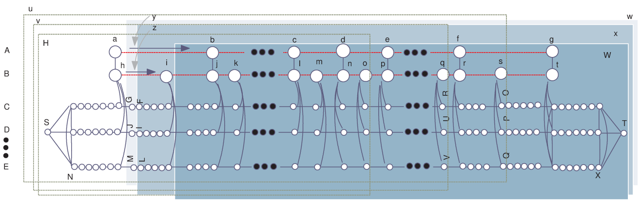
2.4 Proof of Theorem 2.3
Let . Let be the function in the theorem statement. Let be any -error distributed algorithm for computing on . Fix a random string used by (shared by all nodes in ) and consider the deterministic algorithm run on the input of and the fixed random string . Let be the worst case running time of algorithm (over all inputs). We only consider , as assumed in the theorem statement. We show that Alice and Bob, when given as the public random string, can simulate using communication bits in rounds, as follows. (We provide an example in the end of this section.)
Rounds, Phases, and Iterations.
For convenience, we will name the rounds backward, i.e., Alice and Bob start at round and proceed to round , , and so on. Each round is divided into two phases, i.e., when Alice sends messages and Bob sends messages (recall that Alice sends messages first in each iteration). Each phase of round is divided into iterations. Each iteration simulates one round of algorithm . We call the iteration of round when Alice (Bob, respectively) sends messages the iteration (, respectively). Therefore, in each round we have the following order of iterations: , , , , , , . For convenience, we refer to the time before communication begins as round and let and .
Our goal is to simulate one round of algorithm per iteration. That is, after iteration finishes, we will finish the round of algorithm . Specifically, we let
and our goal is to construct a protocol with properties as in the following lemma.
Lemma 2.4.
There exists a protocol such that there are at most bits sent in each iteration and satisfies the following properties. For any and ,
- 1.
after finishes, Alice and Bob know and , respectively, and
- 2.
after finishes, Alice and Bob know and , respectively.
Proof.
We first argue that the properties hold for iteration , i.e., before Alice and Bob starts communicating. After round starts, Alice can compute which contains the states of all nodes in except . She can do this because every node except and has the same state regardless of the input and the state of depends only on her input string . Similarly, Bob can compute which depends only on his input .
Now we show that, if the lemma holds for any iteration then it also holds for iteration as well. Specifically, we show that if Alice and Bob know and , respectively, then they will know and , respectively, after Alice sends at most messages.
First we show that Alice can compute without receiving any message from Bob. Recall that Alice can compute if she knows
- •
, and
- •
all messages sent to all nodes in at time of algorithm .
By assumption, Alice knows which implies that she knows since
Moreover, observe that all neighbors of all nodes in are in . Thus, Alice can compute all messages sent to all nodes in at time of algorithm . Therefore, Alice can compute without receiving any message from Bob.
Now we show that Bob can compute by receiving at most bits from Alice and use the knowledge of . Note that Bob can compute if he knows
- •
, and
- •
all messages sent to all nodes in at time of algorithm .
By assumption, Bob knows which implies that he knows since . Moreover, observe that all neighbors of all nodes in are in , except
In other words, Bob can compute all messages sent to all nodes in at time except
where is the message sent from to at time of algorithm . Observe further that Alice can compute these messages because she knows which contains the states of
at time . (In particular, is a superset of which contains the states of , , .) So, Alice can send these messages to Bob and Bob can compute at the end of the iteration. Each of these messages contains at most bits since each of them corresponds to a message sent on one edge. Therefore, Alice sends at most bits to Bob in total. This shows the first property.
After Alice finishes sending messages, the two parties will switch their roles and a similar protocol can be used to show that the second property, i.e., if the lemma holds for any iteration then it also holds for iteration as well. That is, if Alice and Bob know and , respectively, then Bob can send bits to Alice so that they can compute and , respectively. ∎
Let be the protocol as in Lemma 2.4. Alice and Bob will run protocol until round , where is the largest number such that . Lemma 2.4 implies that after iteration , Bob knows
(note that ). In particular, Bob knows the state of node at time , i.e., he knows . Thus, Bob can output the output of which is output from .
Since is -error, the probability (over all possible shared random strings) that outputs the correct value of is at least . Therefore, the communication protocol run by Alice and Bob is -error as well. The number of rounds is bounded as in the following claim.
Claim 2.5.
If algorithm finishes in time then . In other words, the number of rounds Alice and Bob need to simulate is
Proof.
Let and let . Assume for the sake of contradiction that Alice and Bob need more than rounds. This means that . Alice and Bob requiring more than rounds implies that
| (4) |
It follows that for any ,
| (5) | ||||
| (6) | ||||
| (7) |
where Eq. (5) follows from the definition of , Eq. (6) is because , and Eq. (7) is by the definition of . Therefore, the total number of steps that can be simulated by Alice and Bob up to round is
contradicting Eq. (4). ∎
Since there are at most bits sent in each iteration and Alice and Bob runs for iterations, the total number of bits exchanged is at most . This completes the proof of Theorem 2.3.
Example 2.6.
Fig. 3 shows an example of the protocol we use above. Before iteration begins, Alice and Bob know and , respectively (since Alice and Bob already simulated for steps in round ). Then, Alice computes and sends and to Bob. Alice and Bob then compute and , respectively, at the end of iteration . After they repeat this process for five more times, i.e. Alice sends
Bob will be able to compute . Note that Alice is able to compute , , , without receiving any messages from Bob so she can compute and send the previously mentioned messages to Bob.
3 The pointer chasing problem
In this section, we define the pointer chasing problem and prove its lower bound (Lemma 3.2) which will be used to prove Theorem 1.1 in the next section.
Informally, the -round pointer chasing problem has parameters and and there are two players, which could be Alice and Bob or nodes and , who receive functions and , respectively. The goal is to compute a function starting from and alternatively applying and for times each, i.e., compute where and appear times each. To be precise, let be the set of functions . For any define inductively as
Also define function . The goal of the -round pointer chasing problem is to compute .
Observe that if Alice and Bob can communicate for rounds then they can compute naively by exchanging bits. Interestingly, Nisan and Wigderson [28] show that if Alice and Bob are allowed only rounds then they essentially cannot do anything better than having Alice sent everything she knows to Bob.33 3 In fact this holds even when Alice and Bob are allowed rounds but Alice cannot send a message in the first round.
Theorem 3.1.
[28] .
The pointer chasing problem on .
We now consider the pointer chasing problem on network where and receive and respectively. The following lemma follows from Theorem 2.3 and 3.1.
Lemma 3.2.
For any , , , , , .
Proof.
4 Proof of the main theorem
In this section, we prove Theorem 1.1. An lower bound has already been shown (and is fairly straightforward) in [10]; so we focus on showing the lower bound. Moreover, we will prove the theorem only for the version where destination outputs source. This is because we can convert algorithms for the other two version to solve this version by adding rounds. To see this, observe that once the source outputs the ID of the destination, we can take additional rounds to send the ID of the source to the destination. Similarly, if nodes know their positions, the node with position can output the source’s ID by taking additional rounds to request for the source’s ID. Theorem 1.1, for the case where destination outputs source, follows from the following lemma.
Lemma 4.1.
For any real and integers , and , there exists a family of networks such that any network has nodes and diameter , and any algorithm for computing the destination of a random walk of length requires time on some network .
Proof.
We show how to compute on by reducing the problem to the problem of sampling a random walk destination in some network , obtained by restrict the number of copies of some edges in , depending on input functions and . We let be the family of network over all input functions. Note that for any input functions, an algorithm on can be run on with the same running time since every edge in has more capacity than its counterpart in .
Let and . Note that . For any and , let
That is, , , , , , , , , . Let be the number of nodes in each path. Note that by Lemma 2.1. Denote the nodes in from left to right by . (Thus, and .) Also denote the nodes in from right to left by . (Thus, and .) Note that for any and , and are adjacent to while and are adjacent to .
Now we construct . For simplicity, we fix input functions and and denote simply by . To get we let every edge in have one copy (thus with capacity ), except the following edges. For any , , and , we have copies of edges between nodes and and copies of edges between nodes and . Note that these numbers of copies of edges are always the same, regardless of the input and .
Additionally, we have the following numbers of edges which depend on the input functions. First, specifies the following number of edges between its neighbors. For any , , we have copies of edges between nodes and . These numbers of edges can be specified in one round since both and are adjacent to . Similarly, we have copies of edges between nodes and which can be done in one round since both nodes are adjacent to . This completes the description of .
Now we use any random walk algorithm to compute the destination of a walk of length on by starting a random walk at . If the random walk destination is for some , then node outputs the number ; otherwise, node outputs an arbitrary number.
Now observe the following claim.
Claim 4.2.
Node outputs with probability at least .
Proof.
Let be the path consisting of nodes , , , , , , , , , , , . We claim that the random walk will follow path with probability at least . The node of distance from in this path is and thus the algorithm described above will output with probability at least .
To prove the above claim, consider any node in path . Let and be the node before and after in , respectively. Let and be the number of multiedges and , respectively. Observe that . Moreover, observe that there are at most edges between and other nodes. Thus, if a random walk is at , it will continue to with probability at least . By union bound, the probability that a random walk will follow is at least , as claimed. ∎
Thus, if there is any random walk algorithm with running time on all networks in then we can use such algorithm to solve (with error probability ) in time . Using the lower bound of computing solving in Lemma 3.2, the random walk computation also has a lower bound of as claimed. ∎
5 Conclusion
In this paper we prove a tight unconditional lower bound on the time complexity of distributed random walk computation, implying that the algorithm in [11] is time optimal. To the best of our knowledge, this is the first lower bound that the diameter plays a role of multiplicative factor. Our proof technique comes from strengthening the connection between communication complexity and distributed algorithm lower bounds initially studied in [9] by associating rounds in communication complexity to the distributed algorithm running time, with network diameter as a trade-off factor.
There are many open problems left for random walk computation. One interesting open problem is showing a lower bound of performing a long walk. We conjecture that the same lower bound of holds for any . However, it is not clear whether this will hold for longer walks. For example, one can generate a random spanning tree by computing a walk of length equals the cover time (using the version where every node knows their positions) which is where is the number of edges in the network (see detail in [11]). It is interesting to see if performing such a walk can be done faster. Additionally, the upper and lower bounds of the problem of generating a random spanning tree itself is very interesting since its current upper bound of [11] simply follows as an application of random walk computation [11] while no lower bound is known. Another interesting open problem prove the lower bound of for some value of for the problem of performing walks of length .
In light of the success in proving distributed algorithm lower bounds from communication complexity in this and the previous work [9], it is also interesting to explore further applications of this technique. One interesting approach is to show a connection between distributed algorithm lower bounds and other models of communication complexity, such as multiparty and asymmetric communication complexity (see, e.g., [23]). One particular interesting research topic is applying this technique to distance-related problems such as shortest - path, single-source distance computation, and all-pairs shortest path. The lower bound of are shown in [9] for these types of problems. It is interesting to see if there is an -time algorithm for these problems (or any sub-linear time algorithm) or a time lower bound of exists. The special cases of these problems on complete graphs (as noted in [13]) are particularly interesting. Besides these problems, there are still some gaps between upper and lower bounds of problems considered in [9] such as the minimum cut and generalized Steiner forest.
References
- [1] Lada A. Adamic, Rajan M. Lukose, Amit R. Puniyani, and Bernardo A. Huberman. Search in power-law networks. Physical Review, 64, 2001.
- [2] H. Baala, O. Flauzac, J. Gaber, M. Bui, and T. El-Ghazawi. A self-stabilizing distributed algorithm for spanning tree construction in wireless ad hoc networks. J. Parallel Distrib. Comput., 63(1):97–104, 2003.
- [3] Judit Bar-Ilan and Dror Zernik. Random leaders and random spanning trees. In Proceedings of the 3rd International Workshop on Distributed Algorithms, pages 1–12, London, UK, 1989. Springer-Verlag.
- [4] Thibault Bernard, Alain Bui, and Olivier Flauzac. Random distributed self-stabilizing structures maintenance. In ISSADS, pages 231–240, 2004.
- [5] Ashwin R. Bharambe, Mukesh Agrawal, and Srinivasan Seshan. Mercury: supporting scalable multi-attribute range queries. In SIGCOMM, pages 353–366, 2004.
- [6] Andrei Z. Broder. Generating random spanning trees. In FOCS, pages 442–447, 1989.
- [7] Brian F. Cooper. Quickly routing searches without having to move content. In IPTPS, pages 163–172, 2005.
- [8] Don Coppersmith, Prasad Tetali, and Peter Winkler. Collisions among random walks on a graph. SIAM J. Discret. Math., 6(3):363–374, 1993.
- [9] Atish Das Sarma, Stephan Holzer, Liah Kor, Amos Korman, Danupon Nanongkai, Gopal Pandurangan, David Peleg, and Roger Wattenhofer. Distributed Verification and Hardness of Distributed Approximation. In STOC, 2011.
- [10] Atish Das Sarma, Danupon Nanongkai, and Gopal Pandurangan. Fast distributed random walks. In PODC, pages 161–170, 2009.
- [11] Atish Das Sarma, Danupon Nanongkai, Gopal Pandurangan, and Prasad Tetali. Efficient distributed random walks with applications. In PODC, pages 201–210, 2010.
- [12] Shlomi Dolev and Nir Tzachar. Spanders: distributed spanning expanders. In SAC, pages 1309–1314, 2010.
- [13] Michael Elkin. Distributed approximation: a survey. SIGACT News, 35(4):40–57, 2004.
- [14] Michael Elkin. An Unconditional Lower Bound on the Time-Approximation Trade-off for the Distributed Minimum Spanning Tree Problem. SIAM J. Comput., 36(2):433–456, 2006. Also in STOC’04.
- [15] Joan Feigenbaum, Sampath Kannan, Andrew McGregor, Siddharth Suri, and Jian Zhang 0004. Graph Distances in the Data-Stream Model. SIAM J. Comput., 38(5):1709–1727, 2008. Also in SODA’05.
- [16] Ayalvadi J. Ganesh, Anne-Marie Kermarrec, and Laurent Massoulié. Peer-to-peer membership management for gossip-based protocols. IEEE Trans. Comput., 52(2):139–149, 2003.
- [17] Juan A. Garay, Shay Kutten, and David Peleg. A Sublinear Time Distributed Algorithm for Minimum-Weight Spanning Trees. SIAM J. Comput., 27(1):302–316, 1998. Also in FOCS ’93.
- [18] Christos Gkantsidis, Milena Mihail, and Amin Saberi. Hybrid search schemes for unstructured peer-to-peer networks. In INFOCOM, pages 1526–1537, 2005.
- [19] Amos Israeli and Marc Jalfon. Token management schemes and random walks yield self-stabilizing mutual exclusion. In PODC, pages 119–131, 1990.
- [20] David Kempe, Jon M. Kleinberg, and Alan J. Demers. Spatial gossip and resource location protocols. In STOC, pages 163–172, 2001.
- [21] Jon M. Kleinberg. The small-world phenomenon: an algorithmic perspective. In STOC, pages 163–170, 2000.
- [22] Liah Kor, Amos Korman, and David Peleg. Tight bounds for distributed mst verification. In STACS, pages 69–80, 2011.
- [23] Eyal Kushilevitz and Noam Nisan. Communication complexity. Cambridge University Press, New York, NY, USA, 1997.
- [24] Ching Law and Kai-Yeung Siu. Distributed construction of random expander networks. In INFOCOM, 2003.
- [25] Dmitri Loguinov, Anuj Kumar, Vivek Rai, and Sai Ganesh. Graph-theoretic analysis of structured peer-to-peer systems: routing distances and fault resilience. In SIGCOMM, pages 395–406, 2003.
- [26] Zvi Lotker, Boaz Patt-Shamir, and David Peleg. Distributed MST for constant diameter graphs. Distributed Computing, 18(6):453–460, 2006. Also in PODC’01.
- [27] Qin Lv, Pei Cao, Edith Cohen, Kai Li, and Scott Shenker. Search and replication in unstructured peer-to-peer networks. In ICS, pages 84–95, 2002.
- [28] Noam Nisan and Avi Wigderson. Rounds in communication complexity revisited. SIAM J. Comput., 22(1):211–219, 1993. Also in STOC’91.
- [29] David Peleg. Distributed computing: a locality-sensitive approach. Society for Industrial and Applied Mathematics, Philadelphia, PA, USA, 2000.
- [30] David Peleg and Vitaly Rubinovich. A Near-Tight Lower Bound on the Time Complexity of Distributed Minimum-Weight Spanning Tree Construction. SIAM J. Comput., 30(5):1427–1442, 2000. Also in FOCS’99.
- [31] Ming Zhong and Kai Shen. Random walk based node sampling in self-organizing networks. Operating Systems Review, 40(3):49–55, 2006.
- [32] Ming Zhong, Kai Shen, and Joel I. Seiferas. Non-uniform random membership management in peer-to-peer networks. In INFOCOM, pages 1151–1161, 2005.