Spectrum Sensing Based on Blindly Learned Signal Feature
Abstract
Spectrum sensing is the major challenge in the cognitive radio (CR). We propose to learn local feature and use it as the prior knowledge to improve the detection performance. We define the local feature as the leading eigenvector derived from the received signal samples. A feature learning algorithm (FLA) is proposed to learn the feature blindly. Then, with local feature as the prior knowledge, we propose the feature template matching algorithm (FTM) for spectrum sensing. We use the discrete Karhunen–Loève transform (DKLT) to show that such a feature is robust against noise and has maximum effective signal-to-noise ratio (SNR). Captured real-world data shows that the learned feature is very stable over time. It is almost unchanged in 25 seconds. Then, we test the detection performance of the FTM in very low SNR. Simulation results show that the FTM is about 2 dB better than the blind algorithms, and the FTM does not have the noise uncertainty problem.
I Introduction
Radio frequency is fully allocated for the primary users (PU), but with low utilization rate [1] as low as [2, 3]. The concept of cognitive radio (CR) was proposed so that the secondary users (SU) can occupy the unused spectrum from the PU, therefore improving the spectrum utilization rate. The CR requires the SU to detect the existence of PU in a short time in very low signal-to-noise ratio (SNR), which is spectrum sensing. IEEE 802.22 is the first IEEE working group embedding the CR technology [4] and has triggered lots of research.
Many spectrum sensing algorithms have been proposed. Take the DTV signal sensing for example. Specific features are often defined from the spectral information, such as pilot tone [5], spectrum shape [6] and cyclostationarity [7], etc.. Generally speaking, they are robust and have good performance when it is assumed that those features are universal to all the SUs. However, such assumption is not true in real-life. Fig. 1 shows the DTV spectrum measured [8] at different locations. It can be seen that the spectral features are location dependent, due to different channel characteristics and synchronization mis-match, etc. Therefore, we cannot rely on the pre-determined prior knowledge of signals for spectrum sensing.

Energy based algorithms do not have such problem. Essentially, energy based algorithms require the prior knowledge of noise. However, the noise uncertainty problem [9] will limit the performance of energy based algorithms. Pure blind algorithms have been proposed in [10, 11], such as the maximum eigenvalue to minimum eigenvalue ratio (MME). No noise information is required and the noise uncertainty problem is successfully avoided.
In this paper, we propose to use learned prior knowledge to improve detection performance. The learned prior knowledge is the leading eigenvector derived from the received signal’s sample covariance matrix, using the discrete Karhunen–Loève transform (DKLT). Similar to the terminology of the pattern recognition in machine learning, we define the leading eigenvector as signal feature. We first propose a feature learning algorithm (FLA) to acquire the local feature blindly. Then, we propose a feature template matching algorithm (FTM) which uses the learned feature for spectrum sensing. The leading eigenvector, a.k.a., feature, is optimum in signal representation [12] and most reliable when the distribution of signal is unknown [13]. In analogy with the recognition of pattern features in image and speech, etc., spectrum sensing is the recognition of the PU feature at the receiver. We will show that:
- 1.
Feature is a robust approximation of the non-white wide-sense stationary (WSS) signal against the white Gaussian noise (WGN).
- 2.
Feature has maximum effective SNR.
- 3.
The proposed algorithms are immune to the noise uncertainty problem.
We use both simulated data and real-world data to demonstrate that feature is robust and stable against noise and feature can be learned blindly even in very low SNR. DTV samples [8] are used to compare the detection performance of the FTM and the MME. The simulation results show that to achieve the same detection performance, the minimum required SNR for the FTM is about 2 dB lower than that of the MME, which shows that with the feature as the prior knowledge, the detection performance can be improved.
The paper is organized as follows. The FLA and the FTM are presented in Section II. The theoretical background of the feature is introduced in Section III. Simulation results are shown in Section IV and conclusions are made in Section V.
II Problem Formulation and the Proposed Algorithms
The spectrum sensing problem can be modeled as follows. represents the received signal at the SU, with the PU signal and the WGN. Both and are independent random process with zero mean, but is non-white WSS while is white Gaussian. Assume the frequency bandwidth being sensed is centered at frequency . After Nyquist sampling with period , we can represent the received signal in discrete form: , and . The spectrum sensing problem has two hypotheses: , signal does not exist; and , signal exists. The received discrete form signal under the two hypotheses is therefore as follows:
| (1) |
| (2) |
Two probabilities are of interest. The detection probability, , and the false alarm probability, .
It is assumed that the learning and sensing processes are performed within the channel coherent time, and there is a pre-whitening filter before any processing.
Let , and be random vectors consisting of samples of , and , respectively:
| (3) |
| (4) |
| (5) |
where denotes matrix transpose. Using as the notation for expectation, we have corresponding covariance matrices:
| (6) |
| (7) |
| (8) |
Since and are independent, we have:
| (9) |
Since is WGN, we have:
| (10) |
where is noise variance and is identity matrix.
If we do the eigen-decomposition on the covariance matrix , we can get a set of eigenvalues and eigenvectors , satisfying:
| (11) |
and
| (12) |
In the terminology of pattern recognition, are called features. The process of calculating features is called feature extraction. Since our algorithms only deal with the leading eigenvector, in this paper only is named as feature for brevity.
The exact covariance matrix cannot be derived in practice because we do not know the exact expectation of all the random processes. Alternatively, if we define as the -th sensing segment, we can have an approximated sample covariance matrix by averaging:
| (13) |
Now we use to represent the leading eigenvector of covariance matrix of segment , a.k.a., the feature of segment . We use the intuitive template matching to find the similarity of features between segments and :
| (14) |
Based on the above notations and concept of feature, we propose the FLA and the FTM:
Algorithm 1, the FLA
- 1.
Collect two consecutive sensing segments , , with samples each.
- 2.
- 3.
Extract features and for the corresponding segments.
- 4.
Compute similarity between these two features using (14).
- 5.
If , then feature is learned as .
where is the threshold determined according by the similarity of consecutive noise segments.
Using the learned feature as the prior knowledge, we propose the FTM:
Algorithm 2, the FTM
- 1.
Collect consecutive samples.
- 2.
- 3.
Extract feature of the current segment.
- 4.
Compute similarity .
- 5.
If , then hypothesis is claimed. Otherwise, hypothesis is claimed.
Both and are thresholds to be set according to noise statistics. As will be shown later, and are independent to the noise energy, or the SNR. There is no noise uncertainty problems in setting or .
So far we have proposed the FLA and FTM. In the next section we will show why we use leading eigenvector as feature.
III Theoretical Background
The theoretical background of the FLA and FTM lies in DKLT. It explains why we define feature as leading eigenvector. We follow the description of [14] to get a brief review of DKLT. If we consider a zero mean random sequence , this sequence can be expanded in any set of orthonormal basis functions as:
| (15) |
where the are coefficients in the expansion and “orthonormal” means that the functions satisfy the relation
| (17) |
It is desired to find a particular orthonormal set of functions such that:
| (18) |
Therefore, the coefficients are uncorrelated. Define random vector , coefficient vector , and the matrix
| (19) |
where
| (20) |
From (16), is a unitary matrix such that . (15) and (18) can now be expressed in matrix formulation as:
| (21) |
and
| (22) |
Equation (21) and (22) have the following interpretation. If we consider the sequence as a vector in an -dimensional space, then can be regarded as components of the same vector with respect to a rotated coordinate system. If we choose as the eigenvectors of the covariance matrix:
| (23) |
Then, the resulting satisfy (18). Therefore, the desired set of basis functions in (15) are determined by the eigenvectors of the covariance matrix :
| (24) |
Thus in the new coordinate system, eigenvectors determine the directions, while eigenvalues determine the signal energy in the corresponding directions.
The transformation in (17) with such basis functions is the DKLT, and (15) is called the Karhunen–Loève expansion for the random process. The DKLT is the only transformation that results in (18).
III-A Properties of Feature and DKLT
DKLT has many useful properties. They have been successfully used in principle component analysis (PCA) [15], singular spectrum analysis (SSA) [16] and pattern recognition [17], etc.. We list two of the properties for spectrum sensing.
Property 1:
Equation (15) is the optimal linear approximation representation of the random process if the expansion is truncated to use orthonormal basis functions:
| (25) |
Property 2:
The leading eigenvector is determined by the direction with largest signal energy. For any , will remain almost the same.
Property 2 has a geometric explanation with a two dimensional case in Fig. 2. Assume we have random vectors , where is vectorized sine sequence and is the vectorized WGN sequence. SNR is set to dB. There are 1000 samples for each random vectors in Fig. 2. Now we use DKLT to set the new axes for each random vector samples such that is strongest along the corresponding new axes. It can be seen that new axes for (SNR = dB) and (SNR = dB) are almost the same. axes for (SNR = ), however, is rotated with some random angle. This is because WGN has almost same energy distributed in every direction. New axes for noise will be random and unpredictable but the direction for signal is very robust, as long as .

Property 2 helps us to conclude that among all eigenvectors, only leading eigenvector is most robust against noise. Together with Property 1, we can prove that the leading eigenvector is also optimal approximation of original signal by simply setting to in (25). Moreover, since signal energy/noise energy estimation is not used in the entire process [18], there is no noise uncertainty problem for feature learning.
In another view, the effective SNR on the leading eigenvector is higher than the original SNR. If we do DKLT on and , we have eigenvalues for and for ; eigenvectors for and for . The SNR for is:
| (26) |
Suppose we only use the leading eigenvector to approximate by in (25). Since is white, for all , the SNR for is therefore
| (27) |
The SNR gain after using the leading eigenvector of DKLT is:
| (28) |
Since , . Such SNR gain is optimal [19].
This is the foundation of the FLA and FTM. They use the fact that consecutive features of WSS signal are similar, while consecutive features of noise are random.
III-B Implementation Issue
The major processing part of our algorithms lies in the feature extraction. If we analyze the processing delay of the feature extraction, it can be divided to two steps. First is to compute the covariance matrix in (13) and the other is the eigenvector calculation. Since the computation of can be done in real-time, the major processing delay lies in the eigenvector calculation. In the feature extraction, we only want to know the leading eigenvector and we do not need to do the complete eigen-decomposition, which has computation complexity of . Recently, a fast PCA algorithm for fixed point implementation have been proposed with computation complexity [20], minimizing the processing delay. Being able to compute (13) in real-time is a huge advantage if compared with spectral methods using the fast Fourier transform (FFT). Since FFT can only be calculated when all samples are captured, the computation complexity is . Because usually , the feature extraction has much less delay than FFT. Currently we have implemented the algorithms in field programmable gate array (FPGA) and digital signal processor (DSP) [21, 22].
IV Simulation Results
In this section, we first use show that the signal feature can be extracted under unknown low SNR. Then, real-world captured data is used to show that the signal feature can be learned blindly and is stable over time. Finally, we compare the detection performance of the FTM with the MME in very low SNR, using the same real-world data. In the comparison, same covariance matrix is used, but the FTM has the learned feature as prior knowledge.
IV-A Feature Robustness Test Against Noise
Here we give an example to show feature extraction under unknown low SNR. has constant power spectrum density in the frequency band from MHz to MHz. is the noisy signal with unknown amount of noise. As shown in Fig. 3, no spectral information of can be extracted in the frequency domain. We use the FLA to extract the features from the noisy and the noise free . As can be seen in Fig. 4, those two features are very similar, with similarity as high as . As a result, feature is very robust against noise and there is no noise uncertainty in feature extraction.


IV-B Feature Learning Test with Real-world Data
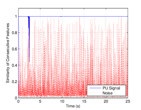
Then we use real world data to demonstrate that the signal feature is very stable over time while the noise feature is random. Field measurements of DTV done in Washington D.C. [8] are used as the PU signal. Simulated WGN samples are used. The captured signal has a duration of about 25 seconds. All synchronization information of the DTV signal is blind to the SU receiver. Receiver SNR and the communication channel between the transmitter and receiver are also unknown. However, we do know that the received SNR is changing at the receiver and the channel has slow fading. We use the FLA to calculate the similarities of consecutive features for both signal and noise in 25 seconds, respectively. We set and . The corresponding duration of each segment is approximately ms. Fig. 5 shows Similarity of Consecutive Features VS Time plot. By setting , for amount of time when the PU signal exists. Moreover, the similarity between the features of the first sensing segment and the last sensing segment is as high as , showing that the signal feature is very stable and almost unchanged in 25 seconds. When the PU signal does not exist, for only amount of time. Sohpisticated learning algorithms will be developed in the feature learning process to obtain the signal feature in a robust and fast manner.
IV-C ROC Curves for the FTM and the MME
We use one segment of the previous DTV data samples as the clean received PU signal and add noise with variance to emulate . In the simulation, the signal feature is the prior knowledge. Sensing time is set to approximately ms with and . WGN is added according to different SNR levels. We compare the results of both algorithms. The MME uses the covariance matrix’s max-min eigenvalue ratio, for detection [10], and uses no prior knowledge. and are set the same for these two algorithms. In the simulation, we perform both algorithms on the same signal and noise and repeat the simulation for times. Fig. 6 shows the VS SNR, with . It can be seen that to reach , the minimum required SNR for the FTM is about dB lower than that of the MME. Note that in our simulations, all set by the FTM to get are very stable for different SNR. This is because is independent of SNR, signal energy or noise energy, and the FTM does not have noise uncertainty problem. Fig. 7 shows the receiver operating characteristic (ROC) curves when SNR = dB. At , FTM has , while MME only has . This shows the advantage of using the prior knowledge.


V Conclusions
Signal feature is location dependent. We propose to learn signal feature blindly and use it for spectrum sensing. We define the signal feature as the leading eigenvector of signal’s sample covariance matrix, because it is a robust approximation of original signal against noise and optimum in effective SNR, based on DKLT properties. We propose the FLA for blind feature learning and the FTM for spectrum sensing with the signal feature as the prior knowledge. Since our algorithms do not depend on SNR or the noise energy, noise uncertainty problem is successfully avoided. We use simulated data and real-world data to demonstrate feature’s robustness against noise and its stability over time. Detection performance of the FTM in low SNR is compared with MME, which is totally blind. Simulation results show that to achieve and , the minimum requried SNR for the FTM is about dB lower than that of the MME.
This is only the beginning of our work. Further research topics include implementation, sophisticated feature learning and quantizing the thresholds, etc. In addition, feature extracted by DKLT is optimum only in the context of linear transforms. When signal has non-linear structures, non-linear methods like Kernel-PCA [23] and manifold-learning [24] can be the next powerful tools to be explored.
Acknowledgment
This work is funded by National Science Foundation through grants (ECCS-0901420), (ECCS-0821658), and Office of Naval Research through two contracts (N00014-07-1-0529, N00014-11-1-0006).
References
- [1] G. Staple and K. Werbach, “The end of spectrum scarcity,” IEEE Spectrum, vol. 41, no. 3, pp. 48–52, 2004.
- [2] FCC, “Spectrum policy task force report,” tech. rep., ET Docket No. 02-155, Nov. 2002.
- [3] D. Cabric, S. Mishra, and R. Brodersen, “Implementation issues in spectrum sensing for cognitive radios,” in Asilomar Conference on Signals, Systems, and Computers, vol. 1, pp. 772–776, 2004.
- [4] “Ieee 802.22 working group on wireless regional area networks,” 2004. http://www.ieee802.org/22.
- [5] C. Cordeiro, M. Ghosh, D. Cavalcanti, and K. Challapali, “Spectrum sensing for dynamic spectrum access of TV bands,” in Second International Conference on Cognitive Radio Oriented Wireless Networks and Communications, (Orlando, Florida), Aug. 2007.
- [6] Z. Quan, S. J. Shellhammer, W. Zhang, and A. H. Sayed, “Spectrum sensing by cognitive radios at very low SNR,” in IEEE Global Communications Conference 2009, 2009.
- [7] A. Dandawate and G. Giannakis, “Statistical tests for presence of cyclostationarity,” IEEE Transactions on Signal Processing, vol. 42, no. 9, pp. 2355–2369, 1994.
- [8] V. Tawil, “51 captured DTV signal.” http://grouper.ieee.org/groups /802/22/Meeting_documents/2006_May/Informal_Documents, May 2006.
- [9] R. Tandra and A. Sahai, “Fundamental limits on detection in low SNR under noise uncertainty,” in Proc. Wireless Commun. Symp. on Signal Process., Jun. 2005.
- [10] Y. Zeng and Y. Liang, “Maximum-minimum eigenvalue detection for cognitive radio,” in IEEE 18th International Symposium on Personal, Indoor and Mobile Radio Communications (PIMRC) 2007, pp. 1–5, 2007.
- [11] T. Lim, R. Zhang, Y. Liang, and Y. Zeng, “GLRT-based spectrum sensing for cognitive radio,” in Global Telecommunications Conference, pp. 1–5, IEEE, 2008.
- [12] S. Watanabe, “Karhunen–Loève expansion and factor analysis: theoreticalremarks and applications,” in Proc. 4th Prague (IT) Conf., pp. 635–660, 1965.
- [13] T. Y. Young, “The reliability of linear feature extractors,” IEEE Transactions on Computers, vol. C-20, no. 9, pp. 967–971, 1971.
- [14] C. Therrien, Discrete Random Signals and Statistical Signal Processing. Englewood Cliffs, NJ: Prentice Hall PTR, 1992.
- [15] L. Smith, “A tutorial on principal components analysis,” Cornell University, USA, vol. 51, p. 52, 2002.
- [16] M. Ghil, M. Allen, M. Dettinger, K. Ide, D. Kondrashov, M. Mann, A. Robertson, A. Saunders, Y. Tian, F. Varadi, et al., “Advanced spectral methods for climatic time series,” Rev. Geophys, vol. 40, no. 1, p. 1003, 2002.
- [17] K. Fukunaga and W. Koontz, “Application of the Karhunen–Loève expansion to feature selection and ordering,” IEEE Transactions on Computers, vol. C-19, no. 4, pp. 311–318, 1970.
- [18] S. Kay, Fundamentals of Statistical Signal Processing, Volume 2: Detection theory. Prentice Hall PTR, 1998.
- [19] J. Makhoul, “On the eigenvectors of symmetric Toeplitz matrices,” IEEE Transactions on Acoustics, Speech and Signal Processing, vol. 29, no. 4, pp. 868–872, 1981.
- [20] A. Sharma and K. Paliwal, “Fast principal component analysis using fixed-point algorithm,” Pattern Recognition Letters, vol. 28, no. 10, pp. 1151–1155, 2007.
- [21] R. Qiu, Z. Chen, N. Guo, Y. Song, P. Zhang, H. Li, and L. Lai, “Towards a real-time cognitive radio network testbed: Architecture, hardware platform, and application to smart grid,” in Networking Technologies for Software Defined Radio (SDR) Networks, 2010 Fifth IEEE Workshop on, pp. 1–6, IEEE, 2010.
- [22] P. Zhang, R. Qiu, and G. Nan, “Demonstration of feature learning based spectrum sensing in cognitive radio.” Submitted, 2010.
- [23] B. Schölkopf, A. Smola, and K. Müller, Advances in Kernel Methods–Support Vector Learning. Cambridge, MA: MIT Press, 1999.
- [24] K. Weinberger and L. Saul, “Unsupervised learning of image manifolds by semidefinite programming,” International Journal of Computer Vision, vol. 70, no. 1, pp. 77–90, 2006.