High Field Studies of Superconducting Fluctuations in High- Cuprates
Evidence for
a Small Gap distinct from the Large Pseudogap
Abstract
We have used large pulsed magnetic fields up to 60 Tesla to suppress the contribution of superconducting fluctuations (SCF) to the ab-plane conductivity above in a series of YBa2Cu3O6+x from the deep pseudogapped state to slight overdoping. Accurate determinations of the SCF contribution to the conductivity versus temperature and magnetic field have been achieved. Their joint quantitative analyses with respect to Nernst data allow us to establish that thermal fluctuations following the Ginzburg-Landau scheme are dominant for nearly optimally doped samples.The deduced coherence length is in perfect agreement with a gaussian (Aslamazov-Larkin) contribution for . A phase fluctuation contribution might be invoked for the most underdoped samples in a range which increases when controlled disorder is introduced by electron irradiation. For all dopings we evidence that the fluctuations are highly damped when increasing or . This behaviour does not follow the Ginzburg-Landau approach which should be independent of the microscopic specificities of the SC state. The data permits us to define a field and a temperature above which the SCF are fully suppressed. The analysis of the fluctuation magnetoconductance in the Ginzburg-Landau approach allows us to determine the critical field . The actual values of and are found quite similar and both increase with hole doping. These depairing fields, which are directly connected to the magnitude of the SC gap, do therefore follow the variation which is at odds with the sharp decrease of the pseudogap with increasing hole doping. This is on line with our previous evidence that is not the onset of pairing. So the large gap seen by spectroscopic experiments in the underdoped regime has to be associated with the pseudogap. We finally propose here a three dimensional phase diagram including a disorder axis, which allows to explain most peculiar observations done so far on the diverse cuprate families.
pacs
74.40.-n, 74.72.-h., 74.25..F-, 74.62.EnI Introduction.
The occurrence of a pseudogap [1] in the phase diagram of high- cuprates has raised many questions which are still intensely debated. Immediately after its discovery, the important issue was to know whether it might be connected to superconductivity (SC). The fact that the onset temperature of the pseudogap has been found quite robust with disorder contrary to has been a strong indication that the two phenomena are not directly related [2].
While this mainly resulted from quasi static NMR measurements in the 1990’s, a large amount of new data using energy and/or wave vector resolved spectroscopies have followed during the last 10 years. STM experiments revealed first that the gap structure detected below in underdoped samples of Bi2Sr2CaCu2O8 (Bi2212) did not totally disappear above, and transforms into a dip in the density of states [3]. From ARPES experiments, it was found as well that a gap structure is observed in the normal state of underdoped samples [4]. The energy gap detected at low was found to match the variation in overdoped samples, i.e. to increase continuously with decreasing doping but continues to increase in the pseudogap state, when decreases [3]. So putting all these observations in perspective has justified the idea that the pseudogap could be a precursor pairing state and not an independent crossover or ordering occuring in the normal state.
This preformed pair scenario has been strengthened by the observations in the underdoped cuprates of a large positive Nernst heat transport coefficient well above up to an onset temperature [5, 6, 7]. This was attributed to vortices and/or phase fluctuations of the superconducting order parameter, along a line suggested initially from finite-frequency conductivity data [8]. Indeed in these compounds with small superfluid density , it has been proposed that is determined by the phase stiffness of the superconducting order parameter and can be much lower than the mean field critical temperature [9]. These experiments, together with the observed diamagnetism above [10, 11] have entertained the idea that a precursor pairing model could be viable to explain the pseudogap. However others suggest that it could be due to a magnetic order, such as stripes, nematic order or orbital currents, which could compete or at least interfere with superconductivity [12, 13, 14, 15].
In a previous report, based on the experimental approach using high magnetic fields to suppress the superconducting fluctuatons (SCF), which will be described in great detail here, we could determine precisely altogether the onset temperatures of the SCF and of the pseudogap within the same set of transport experiments [16]. We have shown there that occurs below the onset of SCF at optimal doping, demonstrating unambiguously that the pseudogap cannot be a precursor state for superconducting pairing and has then to be related to a distinct magnetic order.
This pseudogap issue being settled, it remains that these Nernst experiments evidence that SC pairing extends above , which raises important questions about the nature and high extension of the SCF. Indeed, as for thin superconducting films the SCF are expected to extend well above in 2D systems as compared to the case of classical 3D BCS superconductors where they disappear in a vanishingly small range [17]. This has initiated a large effort to study the extension of SCF in thin metallic films. In particular, it has been demonstrated that a large Nernst signal remains as well above [18], displaying strong similarities on the qualitative aspects with what is observed in the cuprates [19]. Therefore a detailed quantitative study of the SCF in these systems with short coherence length is highly desirable as it might help as well to clear some issues concerning the SC state in high- cuprates.
Since the early days of superconductivity, one of the simplest way to study SCF has been to determine their effect on the electrical conductivity [17]. The fluctuation excess conductivity has been usually well interpreted in the Ginzburg-Landau (GL) formalism in terms of gaussian amplitude fluctuations of the order parameter [20]. Among the different contributions which can be at play, the Aslamazov-Larkin (AL) term either in 2D or 3D appear the most relevant in high- cuprates [21, 22, 23, 24]. However in the majority of experiments reported to date, analyses of the excess conductivity - denoted as paraconductivity in the AL framework- have been limited to optimally doped compounds. Indeed in this case, it has been postulated that the linear dependence of the resistivity observed in the normal state can be extrapolated down to low . The SCF contribution to the conductivity has been then estimated by the deviation from this linear behaviour. As we shall demonstrate in this work such an assumption unavoidably introduces large errors if the normal state resistivity deviates from linear. Also it is unable to give a reliable estimate of the highest temperature at which SCF can be detected as this temperature is a priori imposed by the analysis. Such a criticism is also valid for the magnetoconductance studies in which the normal state contribution is either totally neglected [25, 26, 27, 28] or accounted for by an approximative extrapolation from the high- normal state behavior [29, 30].
Recently we have proposed an original method based on the behavior of the magnetoresistance in high magnetic fields to determine the field and the temperature above which the normal state is completely restored [31]. We have insisted on the fact that was indeed a reliable determination of the onset of SCF. In the present paper we have been able to improve the data accuracy and to extend the measurements for different hole dopings. This allowed us to perform a quantitative analysis of the SCF contribution to the conductivity, and of its and dependence.
After describing the experimental details in section II, we completely determine the normal state variations of the transport properties in section III. We obtain then accurate determinations of the SCF contribution to the conductivity versus and (section IV) both for slightly overdoped and underdoped compounds. The incidence on the SCF of extrinsic controlled disorder introduced by low electron irradiation is studied as well.
In section V we give evidence that is slightly larger than the onset of Nernst effect we have taken before on the same samples [7] and that is comparable to the onset field of SCF deduced from Nernst signal or diamagnetic contributions to the magnetization [11].
We then take advantage of this unique set of accurate data to perform a quantitative analysis of the SCF conductivity (section VI). By confronting these results to Nernst measurements, we do establish then (section VI.B) that, up to , the gaussian AL contribution which decreases as explains quantitatively both data around optimal doping. This approach fails in the case of the most underdoped sample, so that contributions of phase fluctuations might be invoked there in a small range of temperatures above (section VI.C). Above this range, which increases markedly in presence of disorder, gaussian amplitude fluctuations of the order parameter again dominate. In any case, for all the samples studied, we obtain an accurate determination of the dependence of the coherence length and of its limit.
In Section VII, we show that the analysis of the excess magnetoconductivity in the Ginzburg-Landau regime allows us to estimate the upper-critical fields which are found to increase with doping, similarly to the values. From this observation, we can conclude that the superconducting gap increases with doping contrary to the pseudogap which decreases.
In section VIII, we study how the SCF vanish with increasing temperature and magnetic field. We find for all our samples that the SCF magnitude drops sharply at high to vanish near . We point out that the cut-off which must be invoked to explain that behaviour implies that the density of fluctuating pairs vanishes at . Moreover (section VIII.B) the field dependence of the SCF conductivity displays a similar and quite robust exponential dependence in , whatever the hole doping or the quantity of disorder. This behavior again suggests that and are upper limits fixed by the vanishing of the pair formation energy.
We then discuss in section IX the results obtained in the present paper in the context of the large set of data accumulated on the cuprates in the last decade. We draw there conclusions on various important aspects of the normal state and SC properties, and on the incidence of disorder. We shall confirm the independence of the pseudogap from the pair formation and give some clues which might help to clarify the one gap-two gaps dichotomy in these materials.
II Samples and measurements
YBa2Cu3O6+x (YBCO) single crystals were grown using the flux method. Low resistance contacts were achieved by evaporating gold pads in a standard four probe geometry. Subsequent annealings in different atmospheres were performed in order to get samples with various oxygen contents. We have studied four different samples labelled following the values of their critical temperatures taken at the mid-point of the resistive transition: two underdoped samples UD57 and UD85, an optimally doped sample OPT93.6 and a slightly overdoped one OD92.5. The estimate of the hole doping has been done using the parabolic relationship between and [32]. This yields oxygen contents of 6.54, 6.8, 6.91 and 6.95 respectively. Although this is not a totally secure method [33], it helps at least to proceed comparisons between data on similar samples. The resistivity curves of the four different samples are displayed in Fig.1

The magnetoresistance (MR) measurements were performed at the LNCMI-Toulouse in a pulsed field magnet up to 55-60T. The magnetic field was applied along the axis in order to better suppress SC and its polarity was reversed to eliminate by summation any Hall effect contribution to the MR determination.
Controlled disorder was introduced by electron irradiation at low in optimally doped or underdoped samples with K. This type of irradiation provides an efficient way to create point defects, copper and oxygen vacancies, in the CuO2 planes, uniformly distributed throughout the samples [34]. Their effect on the transport and superconducting properties have been extensively studied previously [35, 36, 37]. Whatever the hole doping, we have shown that Matthiessen’s rule is well verified at high temperature - as the high parts of the curves shift parallel to each other. This confirms that the hole doping is not significantly modified. This type of irradiation results in modifications of the superconducting properties very similar to those obtained with Zn substitution [33]. In particular, the rate of decrease which is around - 10K per defect %- in the CuO2 plane (Zn impurities or Cu vacancies) in optimally doped YBCO7 becomes twice larger in underdoped YBCO6.6 [2, 35]
III High Field magnetoresistance: Normal state and SC contributions
Fig.2 shows the tranverse magnetoresistance (MR) curves measured on the OPT93.6 sample for ranging from above to 150K.

Similar curves are obtained for all the samples studied. At high , the transverse MR increases as as better seen in Fig.3. Such a magnetic field dependence has been previously observed in different cuprates for T [38, 39, 40]. More precisely in YBCO, Harris et al. [39] have shown that the weak field magnetoresistance can be expressed as:
| (1) |
where is the cyclotron frequency and is a transverse relaxation time inferred from the Hall angle as . Let us notice here that Eq.1 refers to the orbital MR coefficient which would require the knowledge of , the longitudinal MR . As this latter has been shown to be negligible by Harris et al. [39], we have assumed here that . As Hall constant measurements show that has a quadratic temperature dependence, this explains the behaviour of observed in ref.[39]. The data obtained there in weak magnetic fields are displayed as open symbols in Fig.4, for optimally doped and underdoped YBCO. At sufficiently high temperature, we also observe a variation under high magnetic field in our samples. This is illustrated by the fitting curves in Fig.2(b) or in Fig.3 for the OPT93.6 sample. This indicates that the weak field limit still applies in OPT93.6 up to 55T.
However large departures with respect to this quadratic behaviour appear when is lowered towards . The MR steadily evolves from a quadratic to a nearly linear field dependence. As stated in ref.[31], this evolution can be better viewed in the plots versus of fig.2(b) or Fig.3. There it can be seen that the variation is still visible for fields exceeding a dependent threshold field , which progressively increases with decreasing .

We attribute the initial faster increase of with to the destruction of the fluctuating contribution to the conductivity by the applied magnetic field. In such a case the normal state MR coefficient can then be estimated from the slope of versus at our highest available field (55Tesla). These values of are reported in Fig.4 together with the values determined at low field ( Tesla) on the same sample for . We can see there that the data obtained in high field at low are in continuity with those obtained at higher , which underlines the validity of our analysis, and ensures us that we have effectively completely restored the normal state in high fields for KK for the optimally doped sample. However one can notice in Fig.4 a small upturn of for K (crossed squares) which signals that it is no longer possible to totally suppress the superconducting fluctuations even with 55T at 97K, that is 4K above .

Similar analyses have been done for the OD92.5 and UD85 samples. The data obtained for the UD57 sample are plotted in Fig.5 versus or in a more limited range. One can see in Fig.5(a) the same evolution of the MR as observed for the OPT92.5 sample, from a quadratic to a nearly linear field dependence. However, at K above , the magnitude of the MR is about a factor three larger in the UD57 sample than in the OPT93.6 one. This comes not only from the larger transverse MR in the normal state but also from an enhanced contribution of the SCF as we shall see below.
In such a case one might expect a small saturation of the normal state MR at large field which can be expressed as [41]:
| (2) |

Eq.2 gives better fits to the normal state data displayed as full lines in Fig5(b) for magnetic fields larger than . From these fits one can deduce the values for , which are reported in Fig.4 [42]. They are found here again to be in very good agreement with those obtained in low fields and at higher by Harris et al [39]. The low values of , slightly larger than in our previous report [31] are indeed consistent with this small saturation of the MR in the UD57 sample. This analysis improves the accuracy of the determination of without modifying its magnitude compared to our former data [31].
Let us finally point out that the behaviour of the normal state magnetoresistance shown in Fig.4 is quite similar in the optimal and underdoped case nearly down to and exhibits no sign of the reconstruction of Fermi surface which is observed at lower for the YBCO6.6 [43, 44]. This point will be discussed in more detail in section IX.
IV SCF Contribution to the conductivity
We have shown here above that it is possible to fully recover the normal state conductivity at temperatures slightly above when the pulsed field exceeds . By extrapolating the normal state variations of the resistivity down to zero field, one can thus determine the normal state value of the resistivity at each temperature and magnetic field. Consequently, assuming only that a two fluid model applies, it is straightforward to extract the zero field excess conductivity due to SCF from
| (3) | |||||
In the main studies of superconducting fluctuations in high- cuprates performed up to date, the determination of the fluctuation excess conductivity has been done in optimally doped samples by assuming that the linear dependence of the normal state resistivity observed at high can be extrapolated down to low temperature. As this assumption can introduce some controversies in the analysis of SCF - and we will show below that it is effectively not correct - the study of the fluctuation magnetoconductivity defined as
| (4) |
has been often preferred since no assumption on the dependence of the normal state transport properties is required in this case [25]. Nevertheless, as the corresponding studies have been performed in rather weak magnetic fields, it has been always admitted that the normal state magnetoresistance can be neglected [25, 26, 27, 28], i.e. .
However for the high magnetic fields used in this study, this assumption is not valid and the normal state magnetoconductivity has to be taken into account to deduce the field variation of the SCF contribution [29, 30]. Within a two fluid model, we simply write
| (5) | |||||
From the relations above the measured total variation of the conductivity is therefore
| (6) |
where the normal state conductivity is
| (7) |
This decomposition, which allows us to obtain is illustrated in Fig.6 for magnetoresistance data taken at a fixed temperature K in UD57.
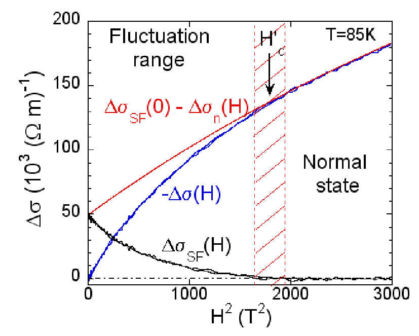
It is worth to emphasize here that the method developed in the present work allows us to determine unambiguously the normal-state contribution in the presence or absence of magnetic field. We have thus been able to analyse separately the variation of with and that of with at each for different hole dopings.
IV.1 Zero field excess conductivity versus T: onset temperature
Let us first consider the dependences of the zero field excess conductivities which are reported in Fig.7 for the four pure samples considered here. One can notice that this quantity dies out very fast with increasing , which allows us to define an onset temperature . Given the noise level of the experiments, we have chosen as in ref.[16] to define as the temperature where is lower than 1 , as indicated in the inset of fig.7.

Let us note that the decrease in with temperature is much slower for the most underdoped sample than for the other ones, so that the extension in temperature of the SCF is larger in this sample than for the other ones.
The variation of with doping is reported in Fig.8. The interesting point is that is only sightly dependent on hole doping and is maximal for optimal doping. We have also reported in this figure the dependence of the pseudogap temperature whose determination has been done simultaneously using the same series of experimental data [16]. The fact that the line crosses the pseudogap line near optimal doping shows unambiguously that the pseudogap phase cannot be a precursor state for the superconducting phase.
The quasi-insensitivity of to doping observed here appears very different from what is observed by Nernst or magnetization measurements in single layer materials such as La1-xSrxCuO4 (LSCO) or La-doped Bi2201 for which the onset temperature of SCF is strongly dependent on hole doping with a sharp maximum in the underdoped region [11]. We will discuss this point in the discussion section IX in conjunction with the effect of controlled disorder.

IV.2 Field variation of the SF conductivity: onset field
In the same way the variation of with magnetic field allows us to analyse how the excess conductivity is destroyed by the applied field. This is exemplified in Fig.9 for UD85 at K. We can see that starts to decrease quadratically with whatever . This dependence is clearly visible at the highest for fields up to 30T. The same behaviour is observed for all the samples studied in the small temperature range which can be explored by our method. One can also notice that the accuracy on decreases with increasing field. This is due both to an increase of the noise induced by the stresses on the magnet at the highest field values and a much reduced data acquisition time in the high field range. This fixes our noise level at about at high fields.
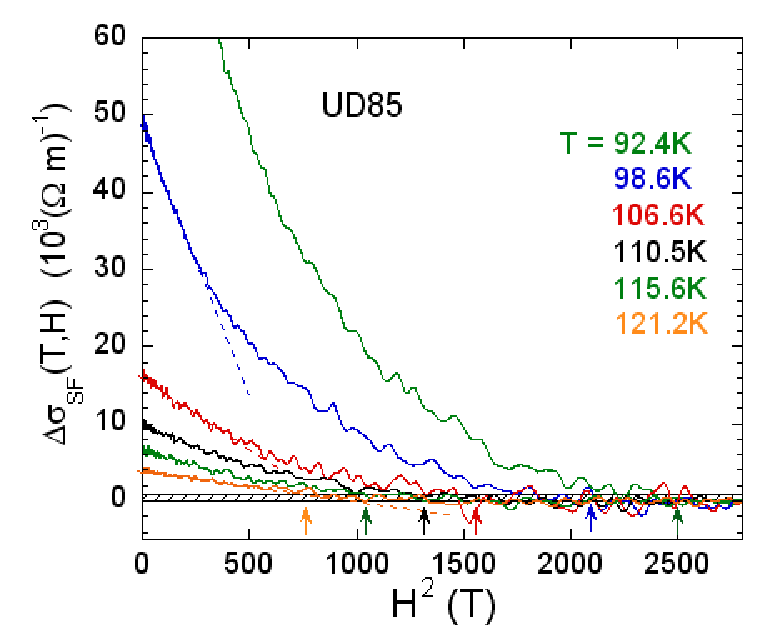
We can thus determine the fields at which becomes smaller than this value. As decreases, it becomes difficult to ascertain that the normal state is fully reached when becomes comparable to the highest available field. This makes difficult to deduce precise values of when they become larger than T.
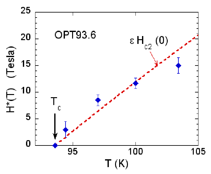
One can see in Fig.10 that drops rapidly with increasing . For all the samples the variation of appears linear near . It is then tempting to use a parabolic variation to fit the data as applied for the critical field of classical superconductors.
| (8) |
The fitting curves displayed as dashed lines in Fig.10 give correspondingly an indication of the field required to completely suppress the SC fluctuation contribution down to 0K. It is clear that increases with hole doping and reaches a value as high as Tesla at optimal doping.

IV.3 Influence of disorder.
In cuprates it is now well established that non magnetic impurity substitutions or in plane disorder are detrimental to superconductivity and strongly depress , the temperature of establishment of 3D superconductivity [33]. However it has been shown as well that the SCF, as seen by Nernst effect, remain at temperatures much higher than the 3D in disordered samples [7]. So, we expect to detect paraconductivity contributions well above in presence of disorder. Let us also notice that increasing disorder decreases markedly , which ensures that a dependence up to 55T is now perfectly verified for the normal state magnetoresistance of irradiated underdoped samples. The magnetoresistivity curves obtained in an UD57 sample in which has been decreased down to 5K are reported in Fig.11 versus or .

It is striking to see that even in this low- sample, a magnetic field larger than 40T is still necessary to totally suppress the superconducting fluctuations at 21K, that is 16K above . Moreover we observe that the term is nearly independent, which might be quite reasonable in this highly disordered sample for which the relaxation time is expected to become rather independent. This confirms that the normal state behavior is totally restored above the threshold field .
The values of are reported in Fig.12(a) for OPT and UD57 samples either pure or irradiated by electron irradiation at low temperature. We notice that the measured SC fluctuation conductivity remains of the same order of magnitude as that of the pure samples in both cases. Using the same procedure as described above, we can also determine for the different samples. The corresponding values as well as the fitting curves using Eq.8 are displayed in fig.12(b).

In the case of the most irradiated UD sample with K, we have been able to nearly completely suppress SC with 55T. The fact that can be rather well fitted by Eq.8 somehow validates the use of this equation to fit our other data. In Fig.13 where the variations of and are plotted versus , one can see that both quantities decrease with increasing disorder. The reduction in nearly follows that in for the underdoped sample while it is slightly larger for the OPT sample. Consequently, when is decreased by disorder, the relative range of SCF with respect to the value of expands considerably. We also observe that decreases linearly with decreasing , but more rapidly for the OPT samples than for the UD57 ones. In both cases, even for samples with very low , magnetic fields as large as 30-60T are still necessary to reach , as can be seen in Fig.13-b.

V Comparison with results obtained by different experiments
We have shown that high field resistivity measurements above allow us to determine the temperature range as well as the extension in magnetic field of the fluctuation excess conductivity. It is thus very interesting to compare our results with those obtained by Nernst effect or magnetic torque measurements that have been developed for more than ten years to probe the presence of SCF above in high- cuprates [11].
V.1 Onset temperature for SCF
The temperature ranges of SCF found here are analogous to those measured in pure high- cuprates by these other techniques. For optimally doped YBCO, K found here is in remarkable agreement with the onset obtained from the diamagnetic response in high fields [11]. The variation with doping is also very similar to that observed in Bi2212 by Nernst effect or diamagnetic measurements [10]. Even though a very small increase of the onset temperature (from 125 to 130K ) is found upon underdoping in this latter case, contrary to our results which show a small decrease (from 135 to 120K) in the same doping range, the important point is that is not found to vary much with doping, contrary to the pseudogap temperature .
It is worth noting that the values of found here for the pure compounds are larger than the onsets of Nernst signal measured previously on the same samples [7]. However one can see in Fig.14, where the determinations of and are compared for the OPT93.6 and UD57 samples, that the criterion used to deduce is much more precise than that for . Indeed a negative dependent contribution of the normal state Nernst signal yields a minimum in , and hides the real onset of SCF. It thus appears that the Nernst effect is not the best probe to detect SCF in the case of YBCO.
In a general way, the measured onset marks the point at which instruments lose sensitivity to detect superconducting fluctuations. This can explain results of a recent report in which the fluctuation excess conductivity measured by Josephson effect between an optimally doped YBCO and an underdoped one with K, drops very fast and is found to vanish at K above [47]. In our case, the excess conductivity of the UD57 sample is still 5% of its normal state contribution at 85K, that is 23K above . Such an explanation might also account for the much smaller fluctuation range determined recently by microwave absorption measurements in YBCO or mercury compounds [48, 49].

We observe that the gap between and is progressively reduced when disorder is introduced in the samples. This is due to the fact that the Nernst signal of normal quasi-particles scales inversely with the scattering rate and thus progressively vanishes with disorder, which permits a more accurate determination of . This results in similar values of and in the most irradiated samples.
V.2 Magnetic field
It is also interesting to compare the values found here to the maximum magnetic field necessary to completely suppress the Nernst or the diamagnetic signals [6, 10]. Although early reports have argued that inferred from Nernst measurements steeply increases with underdoping in Bi2212 [50], more recent studies have shown that this field rather increases with doping in agreement with what we find here for . In particular very large values of have been estimated from torque magnetometry in optimally doped Bi2212 [10]. At , is equal to 90T and is thus quite comparable to the value T deduced here for the OPT93.6 sample from the fitting curve displayed in Fig.10.
One can point out that both values of and are not determined directly by experiments. Here the line is only accessible above and the value of is obtained using Eq.8. For the Nernst (or magnetization) measurements, the values can be only deduced below by taking the extrapolated field at which the Nernst (or diamagnetic) signal should vanish. The fact that similar values of and are observed in optimally doped Bi2212 and YBCO gives some support to these two determinations.
More generally a linear variation of these field values versus or is found when comparing results obtained in low materials like LSCO or La-Bi2201 and our irradiated optimally doped or underdoped YBCO samples as illustrated in Fig.15. As already proposed [7, 31], this relationship between (or ) and (or ) leads us to speculate that the presence of defects, either intrinsically present or intentionally introduced by irradiation will play here a significant role. It is worth noting that the parameters found for the pure UD57 sample obey the same quasi-linear relationship.

However, the results obtained for our other pure samples differ markedly from this behaviour as larger values of with respect to their are found, in agreement with reported value for OP Bi2212 [10]. This is of course directly evidenced in Fig.8 and Fig.10 which show that increases with hole doping while remains essentially the same.
The observation of very large values of well above has been taken as the sign that superconducting fluctuations in all high- cuprates originate from vortex-like excitations in a phase disordered superconductor, rather than fluctuating Cooper pairs [11]. This appears today as an overstatement. Indeed recent experiments have evidenced that the Nernst signal in NbSi films can be explained solely in terms of gaussian fluctuations even in magnetic fields much larger than the orbital upper critical field [18, 69]. Moreover, it has been suggested that the Nernst signal of these films could share some resemblances with those seen in cuprates [19]. It is thus very interesting to compare more quantitatively the evolution of the excess fluctuation conductivity with temperature and magnetic field.
VI Quantitative analysis of the superconducting fluctuations
As already pointed out, a lot of studies have been dealing with the dependence of the paraconductivity in optimally doped high cuprates []. But in most experiments the magnitude of deduced from the data are critically dependent on the behaviour taken for the normal state resistivity, which has been most often taken as linear in . So, we first emphasize here that our method is particularly adapted to perform a precise quantitative analysis of the excess conductivity since our experimental approach allows us to deduce reliably. We have for instance shown in our previous work [16] that the normal state resistivity of the OPT93.6 sample deviates from the linear dependence at K due to the opening of the pseudogap. Consequently, the use of a linear extrapolation for the normal state resistivity would lead to a large overestimate of . To illustrate that, we have therefore mimicked in Fig.16 the difference generated by such an analysis with respect to our reliable determination using magnetoresistance data. It is clear that for such a sample the overestimate of can be quite important. The reliability of the determinations done so far using linear extrapolations of the normal state conductivity can then be put into question in many cases.

VI.1 Contribution of gaussian fluctuations to paraconductivity
The excess fluctuating conductivity is usually analysed in the framework of gaussian fluctuations using the Aslamazov-Larkin theory. As for the Maki-Thompson contribution, which is an indirect contribution arising from the decay of superconducting pairs into quasi-particles and vice-versa, it can be neglected in high- cuprates due to strong pair-breaking effects [52]. In the Ginzburg-Landau theory, the gaussian fluctuations come from the temporal and spatial fluctuations of the superconducting order parameter. The corresponding paraconductivity is directly related to the temperature dependence of , the superconducting correlation length of the short-lived Cooper pairs. Upon cooling down to , is expected to diverge with a power-law dependence given by:
| (9) |
where is the zero-temperature coherence length and for . Depending on the relative values of the temperature dependent perpendicular coherence length and of the layer spacing , the paraconductivity can evolve from a 3D behavior in the immediate vicinity of towards a 2D behavior at larger temperatures [21]. The paraconductivity can be expressed more generally by using the Lawrence-Doniach (LD) theory of layered superconductors as [53]:
| (10) |
where the coupling parameter with . Sufficiently far from , one expects and Eq.10 reduces to the well-known 2D Aslamazov-Larkin expression:
| (11) |
The only parameters in this expression are the value of the interlayer distance and the value taken for which can have a huge incidence on the shape of the curve especially for .
We have plotted the variation of for the four different hole contents as a function of in Fig.17.

For all the samples except UD57, it is striking to see that our experimental data collapse on a single curve. Moreover we can see that the data can be fitted reasonably well by the Lawrence-Doniach expression (Eq.10) in the small temperature range if one takes Å. We have assumed here, as usually done, that the CuO2 bilayer constitutes the basic two-dimensional unit, and is then taken as the unit-cell size in the direction: Å. This is a strong indication that the excess fluctuation conductivity is mainly due to gaussian fluctuations in these different compounds. One can see that all the curves in Fig.17 bend downwards very rapidly for . This behavior has been pointed out earlier in different fluctuation studies on YBCO [54, 55, 56]. It has been proposed that this could be due to the limitations of the Ginzburg-Landau theory in these compounds with very short coherence lengths. We will discuss this point in more details in paragraph VIII.A.
It is clear that the situation is completely different for the UD57 sample for which is found to be about a factor four larger than for the other dopings. This points to an additional origin of SCF in this underdoped sample. In fact we find that the data for this sample can be reconciled with the unique curve found for the other samples by using an effective value different from the actual . This is illustrated in fig.17 in which the data of UD57 are also reported versus using =72K which is much larger than the actual K.
The same conclusion has been proposed in ref.[57] to account for the Nernst signal at high in underdoped LSCO which was found too large to be explained only by Gaussian fluctuations. In the phase fluctuations scenario proposed by Emery and Kivelson [9], this would mean that the actual is suppressed from the mean-field transition temperature by phase fluctuations. However gaussian fluctuations are still expected above this temperature. Thus it appears reasonable here to assimilate our effective to . Let us notice that this conclusion is in contrast with that argued from paraconductivity measurements in underdoped LSCO samples, in which a description in terms of a 2D AL approach has been proposed to completely account for the experimental data [58]
It is also interesting to consider the effect of disorder on the paraconductivity. As seen in Fig.18, the curve found for the disordered optimally doped sample with K nearly falls on that of the pure sample, indicating that here again it is possible to explain the SCF in the framework of the AL theory. However, this is not the case for the underdoped samples, since their curves are shifted towards larger values of with increasing disorder. So the introduction of disorder appears to accentuate the difference with the behavior expected from a GL approach. This will appear more clearly in the next paragraph.

VI.2 Nernst effect
In view of the results found above for the paraconductivity, we have found important to analyse as well our Nernst results taken on similar samples [7] along the same lines. The evolution of the off-diagonal Peltier term [59] has already been recalled in Fig.14 for the pure OPT and UD57 samples. In the 2D Ginzburg Landau approach, has been found to follow the simple expression [57]:
| (12) |
that shows that is related to the spacing between the layers and the Ginzburg-Landau coherence length in the ab-plane . Consequently, according to Eq.11, there is a simple linear relationship between and :
| (13) |
whose slope provides a direct determination of the zero temperature coherence length . Let us point out that, had we taken the LD term in Eq.12, it would have been eliminated as the spacing between layers in this expression 13.
We have tested this relationship first for the optimally doped case and the data are plotted in Fig.19(a). At high a negative normal state contribution to the Nernst signal [7], apparent in Fig.14 (similar to that seen by Daou et al. [60]) dominates that due to SCF. Nevertheless near , this negative counterpart is overcome by the sharp increase of the positive SCF contribution so that the linear relation of Eq.13 is reliably verified, as can be seen in Fig.19(a). The linear slope found there near results in a value nm after correction for the estimated small negative Nernst contribution.
Using the relationship between and
| (14) |
this would lead Tesla, a value which resembles that of determined above. Consequently, we can conclude that, in optimally doped YBCO, the paraconductivity and the Nernst signal above are consistent with each other and can be interpreted in terms of gaussian fluctuations only, with nm.

For the UD57 samples, pure and irradiated with K, the corresponding data are plotted in Fig.19(b). The same analysis can be done for the pure UD57 sample in the high range (above , that is low values of ) where a gaussian regime is expected to be restored. As can be seen in Fig.14, the normal state contribution of the off-Peltier term is positive in this case, so the linear fit of the raw data will give a slightly overestimated value nm. This would correspond to T, similar here again to T estimated for this compound.
This conclusion is clearly no longer valid at lower temperatures, near , as the SCF contribution of the off-diagonal Peltier term markedly increases with respect to this linear relation. This confirms our previous conclusion that the Nernst data in the pure UD57 sample are not consistent with gaussian fluctuations for K. We furthermore evidence that, in this range, the positive contributions to the Nernst signal are greatly enhanced with respect to the SCF paraconductivity.
VI.3 Contribution of phase fluctuations
As an explanation in terms of gaussian fluctuations is not sufficient to account for the excess conductivity in the UD57 samples, either pure or disordered, it is natural to address the possible role of phase fluctuations. Indeed in these systems with low carrier density and/or high level of disorder [9], the low superfluid density is expected to lead to phase fluctuations below the mean-field transition temperature . It has been proposed that the superconducting transition is caused by the proliferation of vortices which destroy long-range phase coherence similarly to that predicted for the Kosterlitz-Thouless transition (KT) [62]. This would result in a phase-incoherent state with a finite pairing amplitude between and . In the framework of the 2D KT transition, the excess conductivity is expressed as:
| (15) |
where the coherence length is now related to the vortex density through . It turns out that a similar relation holds also in the AL regime as shown above (see Eq.11), but here is expected to diverge exponentially at . An interpolation formula between these two regimes has been proposed initially by Halperin and Nelson [63]. More recently, Benfatto et al. [64] have revisited this problem by means of a renormalization group (RG) approach and have established a direct correspondence between the parameter values used to describe the BKT fluctuation regime and the reduced temperature between and defined by:
| (16) |
They propose an interpolation formula for which is formally similar to that of Halperin and Nelson:
| (17) |
but where the parameters and are now obtained from the numerical RG calculations of the correlation length near the transition, so that is close to unity and given by where measures the deviation of the vortex core energy with respect to the conventional value in the XY model.
We have thus tried to fit the data obtained for the SCF conductivity in the pure and irradiated UD57 samples in Fig.20, where are plotted versus in a semi-log scale. Only the very small number of data between and the sharp downturn of are pertinent in such fits. In the pure UD57 sample, within the foregoing analysis, a natural upper limit for the fit would be K which could be assimilated to . We indeed find that the three significant data permit to obtain values for and for which the fitted function deviates from the data above . If we take the same criterion to estimate in the other samples, we get the values for reported in table 1. As expected, we find that increases with disorder, more than a factor 10 between the pure and the most irradiated sample.
It is clear that the limited analysis done above is not sufficient to prove per-se that the increased magnitude of the SCF can be attributed to phase fluctuations. Both phase fluctuations and amplitude fluctuations could be emphasized altogether, as claimed by some authors [65]. Hopefully with the larger pulse fields which become available now, more data points between and could become accessible and would allow to better test the applicability of Eq.17 and to get reliable determinations of the different parameters. The fast suppression of the SCF at high , similar to that found for the optimally doped samples, will be discussed in section VIII.A.
| samples | pure | irr1 | irr2 |
| (K) | 56 | 26.5 | 4 |
| (K) | 72 | 39 | 30 |
| 0.22 | 0.5 | 2.6 | |

VII Fluctuation magnetoconductivity
It is also interesting to look more carefully on the way the SCF are suppressed by the magnetic field. Let us recall here that the dependence of the magnetoconductivity with and has been extensively studied in high- cuprates [25, 26, 27, 28, 29, 30]. This has been often preferred to the study of paraconductivity as its value is often considered as weakly dependent on the normal state magnetoconductivity. In fact this is not really correct even at low magnetic fields since both quantities display inital variations as shown in Fig.6. It is thus necessary to subtract the normal state contribution as expressed in Eq.6 and to consider the difference
| (18) | |||||
Within the GL theory, the evolution of the fluctuating magnetoconductivity with comes from the pair-breaking effect which leads to a suppression. Different contributions must be taken into account to completely explicit the effect of a magnetic field on the excess conductivity [66, 29, 67, 26, 27, 28]. Nevertheless it seems legitimate to neglect the Maki-Thompson contribution which already does not contribute to the paraconductivity in zero field. The Aslamazov-Larkin contribution is the sum of two different contributions resulting from interactions of the magnetic field with the carrier orbital (ALO) and spin (Zeeman) degrees of freedom. The former vanishes for applied fields in the ab plane, and the remaining Zeeman term is usually found much smaller than the ALO term for and low enough magnetic fields [29, 27].
In the layered superconductor model the ALO fluctuation magnetoconductivity can then be written as [29, 27]:
| (19) |
Here , where is the coupling parameter defined in VI.A and is the momentum parallel to the magnetic field H. is the di-gamma function, and . This expression assumes that the temperature dependence of is simply given by:
| (20) |
This holds as long as the behavior in magnetic field is set by the size of . But when the magnetic field becomes large enough, the magnetic length enters into play and overcomes the variation of . The crossover between these two regimes occurs for a field such as
| (21) |
This magnetic field defined above has been called the ”ghost critical field” by Kapitulnik et al [68] as it mirrors the upper critical field defined below . For , the variation with is governed by the magnetic length as recently evidenced by Nernst measurements in SC disordered films [69].

In order to analyse the experimental data, we use the procedure described in ref.[68]. We first determine the only adjustable parameter by matching the low-field part of the data for all values of . We then introduce the higher field values of computed from Eq.19, which allows us to define the ghost field above which a deviation from the experimental data occurs.
This is illustrated for the OPT93.6 sample in Fig.21 where the evolution of is plotted versus at different temperatures ranging from 94.4 to 103.4K, corresponding to values from 0.0085 to . In this temperature range, good fits of the low-field data can be achieved with T. One can also see that the agreement deteriorates at larger fields with increasing temperatures. This is in reasonable agreement with what is expected from Eq.21, as can be seen in Fig.22. So, the data follow unambiguously the GL analysis and enable us to determine reliably.
At higher , beyond the GL range deduced from the zero field SCF conductivity data, the low field data cannot be matched with Eq.19 with the same value of . One may artificially find a better agreement by increasing with increasing temperature, but this is meaningless and only confirms that Eq.19 is no longer valid beyond the GL region. So the choice of temperature range used to fit the data can severely affect the deduced value of . This might explain why previous attempts to deduce from magnetoconductivity data give contrasting results for optimal doping (those of ref.[29] are in better agreement with ours than those of ref.[30]).
We could repeat the same procedure for all the dopings studied here, which leads to values of indicated in table 2. In the case of the UD57 sample, the analysis has been performed by assuming that the mean-field temperature is 72K, as indicated above. As seen in Fig.23, it is still possible to fit the low-field data reasonably well using Eq.19 in a range which is found to slightly exceed the GL regime.
We notice that the value determined in this way are surprisingly close to those obtained for in a totally different way in section IV.B, which are reported as well in Table 2.

| samples | UD57 | UD85 | OPT93.6 | OD92.5 |
| (T) | 90(10) | 125(5) | 180(10) | 200(10) |
| (T) | 86(10) | 115(15) | 155(10) | 207(10) |
| (nm) | 1.9 | 1.60 | 1.33 | 1.26 |
| (meV) | 46 | 50 | 66 | 69.5 |
The very important result of this analysis is to unambiguously show that increases and thus decreases with increasing doping in YBCO.
The coherence length is related to the superconducting gap through:
| (22) |
with for s-wave superconductors. By assuming that the Fermi velocity is weakly dependent on doping as found in different cuprates [70] and equal to [71] m.s-1, we obtain the values of indicated in Table 2. Independently of the precise value of , our results demonstrate that the superconducting gap is closely related to in the doping range to considered here.
Recent STM measurements have shown that meV for an overdoped Bi2212 sample with K [73], yielding a ratio . A similar ratio is also found for the ”small” gap meV identified in the STM spectra of an underdoped Bi2201 sample with K [74]. We notice that for in Eq.22, the data of Table 2 would also correspond to a similar gap magnitude whatever the doping. This is a strong indication that the gap determined here can thus be assimilated to the ”small” gap detected recently by different techniques [72].
VIII Suppression of SC fluctuations by temperature or magnetic field
We shall consider now more specifically the sharp decrease of SCF found versus temperature in Fig.17 and the onset of SCF at and .
VIII.1 Temperature
Within the Ginzburg-Landau description, there is a priori no upper temperature limit for the existence of fluctuations, that are expected to survive far above in the normal state. However it has been pointed out very early that a rapid attenuation of the fluctuations may occur for in short coherence-length systems, as the GL theory can be put into question when becomes comparable to the zero-temperature in-plane coherence length [54, 55, 56]. It has been first argued that a short-wavelength cut-off should be taken into account in the fluctuation spectrum. An extension of the AL theory in the two dimensional case taking this cut-off into account [75] gives a dependence of the superconducting fluctuation conductivity as:
| (23) |
where the function matches the first order expression up to but deviates then to reach the asymptotic limit [76] . Our data can be fitted using the function up to . But as shown in Fig.24, it then drops much faster well below the expected dependence, above temperatures corresponding to coherence lengths .

Other authors have proposed that a ”total-energy” cut-off [78, 79] should be more appropriate to describe the evolution of the paraconductivity in the high region. They assigned its origin to the intrinsic constraint that SCF cannot survive when the coherence length becomes comparable to the superconducting coherence length . They proposed then to mimic this effect using a phenomenological expression which can be transformed into
| (24) |
where . Our data in YBCO unambiguously allowed us to demonstrate that SCF are heavily, if not totally, suppressed at high , which allowed us to define a temperature above which their detection becomes nearly impossible. This value could in principle be obtained as well using the phenomenological Eq.24. However this equation privileges the cut-off behaviour and does not reproduce the low regime where we have established the validity of the Ginzburg-Landau approach.
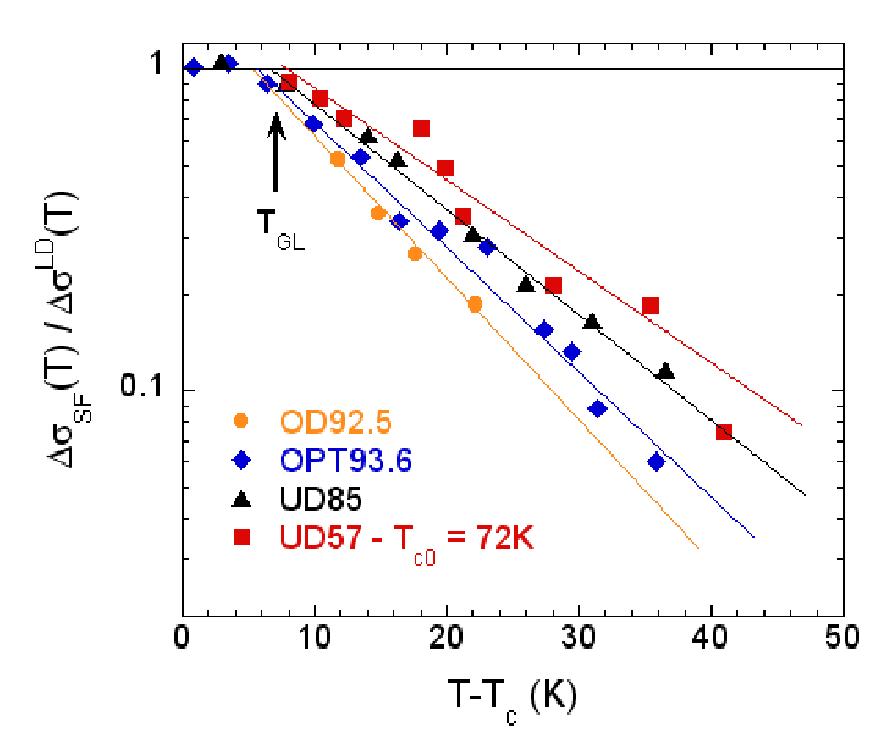
In order to analyse more precisely the attenuation of the superconducting fluctuations with temperature, we have therefore plotted in Fig.25 the values of normalized to those expected from the LD formula versus in a semilogarithmic scale. For all the samples, we observe that the SCF conductivity vanishes exponentially for , as
| (25) |
Here, , the upper temperature for the Ginzburg-Landau regime exceeds of about 5 to 7K. Let us recall here that, for the most underdoped sample, we have replaced by K, the mean field temperature determined above. The exponential decay rate of the SCF increases from 10 to 15K with decreasing doping.
In our previous report [31], we had proposed that the total suppression of SCF in the cuprates could be associated with an intrinsic ultimate possibility to thermally induce pairs in these systems. The simultaneous analysis of the Nernst, paraconductivity and magnetoconductivity data allow us to underline that is intrinsically very small in these compounds and of the same order as the mean distance between the hole carriers, that is about 10Å for instance in optimally doped cuprates with a hole content of 0.16 per Cu. Therefore pairing with shorter coherence length scale would correspond to a thermal excitation of isolated Bose pairs. The total suppression of paraconductivity and Nernst signals above therefore means that the density of such excited pairs drops to zero already at . This fits with the idea that the energy of fluctuations which can be thermally excited is bounded with a sharp cut-off at an energy .
In usual BCS materials, for which the density of carriers per atom is of the order of unity, is large enough with respect to the atomic distance , so that SCF fluctuations could be thermally excited as long as , which agrees with the observation that SCF survive up to at least in amorphous superconducting films [18].
The existence of such a sharp cut-off at is not restricted to pure samples but also applies for disordered ones. This similarity appears very clearly in Fig.20 for the underdoped irradiated samples where the excess conductivity above nearly parallel that of the pure sample and vanish exponentially with the same decay rate.
It is quite intriguing to see this quasi ”universality” of the SCF attenuation in a range where one would rather expect a response highly sensitive to the peculiar features of the systems of interest. This exponential decay means that a range of the order of is universally required to suppress the fluctuations above , or in the underdoped cases. Independently of the physical meaning of this representation, this shows that the SCF vanish similarly with increasing for all the hole contents. This confirms that the pseudogap state has no specific incidence on the range of SCF. This observation contradicts the recent proposition [80] which attributes the rapid suppression of superconducting fluctuations evidenced by Nernst effect and conductivity measurements in underdoped LaSrCuO [6, 58] to the presence of the pseudogap. All the detailed analysis of the data proposed here rather substantiates the conclusion done previously from the simple comparison of the and lines [16] that these two lines are underlining two independent phenomena in the phase diagram of cuprates.
VIII.2 Magnetic fields
In the analysis of the fluctuation magnetoconductivity done above, we have been able to fit the data using Eq.19 as long as for which the Ginzburg-Landau coherence length becomes comparable to the magnetic length .

Well beyond the Ginzburg-Landau regime, for , where the coherence length is strongly reduced by temperature, we expect that the fluctuation magnetoconductivity cannot be described any longer by Eq.19. Some data taken in this regime are illustrated in the case of the UD85 sample in Fig.26(a).
There it can be seen that the excess conductivity appears to decay exponentially with the magnetic field as
| (26) |
This sharp exponential decay confirms that can indeed be reliably defined and is not so dependent on the criterion used (we defined it here and in ref.[16] for )
In order to better visualize how the SCF are suppressed by magnetic fields in the whole range, we have then plotted versus in a semilogarithmic scale in Fig.26(b) for the UD85 sample. For the lowest temperatures, we find that Eq.19 applies with T as long as . It is intriguing to see on this plot that the decay of evolves then smoothly towards an exponential behaviour with nearly the same value of as found at higher temperatures. The same type of evolution is observed for all the samples, pure or irradiated. remains nearly constant whatever the temperature, doping or disorder level with T as can be seen in Fig.27.

To our knowledge, such an exponential suppression of the magnetoconductivity has never been reported experimentally nor predicted theoretically.
IX Discussion and conclusions
We have done here a set of measurements where the normal state magnetoresistance of YBa2Cu3O6+x could be followed down in temperature from the high totally non superconducting state. This allowed us to monitor the progressive advent of fluctuation contributions to the conductivity above . We could not therefore study the close vicinity of , that is the 3D critical exponents. However this experiment quite uniquely allowed us to study the variation of SCF from the 3D to the 2D higher regime. We could evidence that the Ginzburg Landau regime applies near for optimally doped samples, while for underdoped ones phase fluctuations might play a role in a narrow range above . Above those ranges the SCF are highly damped, which reveals the intrinsic microscopic limitations of the pairing at high temperatures. We have also evidenced that disorder increases the phase fluctuation regime above . We shall summarize below the most important conclusions and questions which arise from this work.
Normal state properties in the pseudogap phase
In section III we definitely evidenced that a 60 tesla field is not sufficient to suppress totally the 3D superconductivity at in the pure 123 phases, even for underdoped samples with K, so that the normal state transport properties are only accessible above. The SCF could only be suppressed fully with 60 tesla in the presence of strong disorder reducing down to K.
In the pure UD57 sample we had demonstrated that the resistivity keeps a metallic behaviour at low in large applied fields [31]. This hole content is slightly lower than that on which maximal quantum oscillations have been observed at low and high applied fields [43]. From the negative Hall effect detected in these experiments [44], a reconstruction of the Fermi surface with the appearance of an electron pocket has been proposed. Here we evidenced that the simple relation between the magnetoresistance and the Hall effect which had been established above K in the past [39] has a validity which extends nearly down to , without any singular behaviour both for this YBCO6.6 composition and for an optimally doped sample. This is in rather good agreement with the fact that, for underdoped K samples, the high field Hall constant becomes negative only below the zero field , and that the Fermi surface reconstruction only arises deep into the SC state, in fields which are however insufficient to totally suppress the SCF.
Ginzburg-Landau regime: critical fields and gaps
For samples around optimal doping, the quantitative comparative analysis of the measured SCF contribution to the zero field conductivity and of the off-diagonal Peltier term has been found in total agreement with the GL approach for 2D Gaussian order parameter fluctuations (section VI.B). The data perfectly fit the leading order 2D Aslamazov Larkin contribution up to using the lattice constant as the mean spacing between the CuO2 bilayers. It can be fitted as well up to if higher order corrections are taken into account. This analysis allows us to deduce values of and of versus doping.
The analysis of the fluctuation magnetoconductivity in this GL regime allows us to determine independently in section VII. The good agreement between these different values establishes the perfect consistency of our data analyses. A very important result obtained here is that the deduced superconducting gap increases smoothly with increasing hole doping from the underdoped to the overdoped regime.
Let us recall that energy resolved spectroscopies have evidenced spectral gaps in the SC state which increase with decreasing doping while here we find a gap which rather follows the same trend as . For overdoped samples the local density of states (LDOS) has coherence peaks [3, 73] and exhibits the dependence expected for wave pairing, which distinguishes the nodal and antinodal regions [4]. Above a small dip in the LDOS remains and has been assigned to the pseudogap, but should be attributed to SCF, as we have shown that in this range the pseudogap disappears [16].
But in the underdoped cases a large gap is found to persist then well above , while at low energies the LDOS becomes nearly independent of local disorder [81, 74]. A large debate has been raging recently as various spectroscopy data have suggested that a smaller gap exists, visualized in the nodal regions by Raman spectroscopy [82] or obtained by discriminating different spectral weights in the ARPES or STM spectra [83, 74]. Our deduction here, that an important SC property deduced from thermodynamic considerations, that is the critical field , is governed by a gap which follows , reinforces then the idea that the pseudogap is connected with the large gap detected by STM and ARPES on cuprate sample surfaces in the underdoped regions of their phase diagram. Conversely it can be seen that the gap magnitudes deduced from our data scale quite nicely with the smaller gaps obtained by STM [73, 74].
Phase coherence and phase fluctuations
For the K underdoped sample, well into the pseudogap phase, the SCF paraconductivity and Nernst coefficient are found in section VI.C both much larger than expected for Gaussian fluctuations in a range of temperatures of the order of 15K above , which points for the occurrence of phase fluctuations . This range increases markedly if disorder is used to decrease and can become as large as 40K when has been depressed down to K. These results are therefore consistent with the proposal done by Emery and Kivelson [9], that in the underdoped regime, controlled disorder reduces the phase coherence. The regime where phase fluctuations might play an important role occurs then between the 3D up to a mean field temperature which we can assimilate to . In this limited range we do not have sufficiently accurate measurements, nor theoretically established firm criteria to go beyond qualitative observations.
We noticed however that the Nernst signal is more enhanced than the excess fluctuation conductivity with respect to expectations for Gaussian fluctuations. More work, both theoretical and experimental, is required to decide the possible importance of vortex contributions to the Nernst effect in this phase fluctuation regime and/or other possibilities such as the enhancement of SCF by AF spin fluctuations [84]. However this enhancement of Nernst effect with respect to excess conductivity decreases for . So while it has been recently proposed that Nernst measurements were among the best approaches to probe the extension of the SCF above [6], we demonstrated here that those are indeed not as powerful as expected initially for pure YBCO as they are limited by the need of an independent determination of the normal state Nernst coefficient. The latter is not as small as could be anticipated from the Sondheimer cancellation rule which applies only for classical metals [85, 86]. For the conductivity measurements, our approach using high fields and the former knowledge of the high magnetoresistance permitted to circumvent the corresponding difficulties, so that the SCF could be followed until they are fully suppressed at high .
Suppression of SCF at high and pairing energies
We have evidenced that in all samples, pure or disordered, and for all dopings, the SCF sharply decay with increasing or , in the ranges where SC gaussian fluctuations are dominant. In section IV.B, we could then deduce for all the samples a curve ending at , which delineates the plane region beyond which SCF are totally suppressed.
In section VI.A, the SCF are found to be much more rapidly depressed than in thin films of classical s-wave metallic superconductors for which SCF are detected even for [18]. This provides a strong support for our preliminary suggestion [31] that the curve delineates the regime where microscopic considerations specific to the cuprate physics prohibit SC pairing. We propose in section VIII.A that the spatial pair extension at high is limited by the actual density of carriers available for pairing, so that a lower bound of could be linked with the distance between doped holes.
The suppression of the fluctuation conductivity is found in section VIII to display a phenomenological exponential decay in and , with values of and which are not markedly dependent on the doping and disorder. This suggests as well that there is a sharp energy cut-off at which is shifted by the magnetic energy increase which scales with . The energy balance is such that SC pairs cannot be thermally excited any more above or . Let us notice as well that the extrapolated values of have been found to be nearly identical to those obtained for , which gives confirmation that both are connected with the pairing energy. All these consistent deductions give weight to the present analysis.
Influence of disorder and generic PD of cuprates
It has been found by STM that cuprates (or at least Bi2212 surfaces) displayed a short range disorder, visible for instance as a spatial distribution of spectral gaps [87]. These observations have been questioned as being non generic, as NMR data indicate that YBCO is not as disordered [88], hence the metallic behaviour observed for YBCO6.6 [31]. This has justified our use of YBCO to study the pure cuprate behaviour and the incidence of disorder [36]. We have as well shown that controlled disorder affects drastically the transport properties. Indeed similar upturns of have been found for controlled disorder in YBCO and in some pure cuprate families, which indicated the occurence of intrinsic disorder in those families [46].
The influence of such disorder on SCF has been thoroughly studied in section IV.C and we have shown that the local pair formation underlined by the line is only moderately affected, while the bulk , that is the SC pair coherence can be severely reduced by disorder. Our results allow us to draw important conclusions on the cuprate phase diagram which we had specifically emphasized in a preliminary report [16]. We could determine that the pseudogap line crosses the line at optimal doping, which establishes unambiguously that the pseudogap is not the onset of pairing. The results presented here re-enforce completely this conclusion as the fluctuations are similarly limited in field and temperature independently of the pseudogap, though they are enhanced in magnitude in the underdoped regime.
We want to insist here that specific effects induced by disorder are certainly at the origin of many confusions in the study of HTSC. It is interesting to mention here very recent STM data taken on classical metallic films in presence of large disorder [90]. LDOS measurements reveal strong spatial inhomogeneities of the superconducting gap. The remarkable finding is that the gap magnitude is not much affected when increasing through while the coherence peaks in the one-particle LDOS disappear. While pairs should be thermally excited and fluctuating above , those appear to be localized by disorder as preformed pairs. The authors call ”pseudogap” the reduction of LDOS detected above [91]. This gap, which is induced by superconducting fluctuations and favored by the vicinity of the superconductor insulator transition in the most disordered samples, has no relation with the situation encountered in clean HTSC, for which the pseudogap is not due to SC pairing and has no connection whatsoever with disorder [33]. This experiment is however quite striking as it demonstrates how disorder can produce phenomena which can be easily confused with the pseudogap which characterizes the properties of clean cuprates.

This reinforces our insistence that the cuprate phase diagram has to take into account the presence of disorder, which we have suggested for long to explain the anomalously low optimum value in some cuprate families. This 3D phase diagram that we anticipated from previous results probing the metal insulator transition [46] and from the recent comparison of and is displayed in Fig.28. There, in the pure high systems the occurence of SCF and the difficulty to separate the SC gap from the pseudogap in zero field experiments justifies that the line could often be mistaken as a continuation of the line. It can be also seen there that the respective evolutions with disorder of the SC dome and of the amplitude of the SCF range explains as well the phase diagram often shown in a low cuprate family such as Bi2201 [89]. There both and might appear well above the shrunk SC dome probably because the actual concentration of carriers is not determined independently but just mapped from the shape of the SC dome [32]. Finally for intermediate disorder, the enhanced fluctuation regime with respect to illustrated in the initial Nernst measurements performed in the La2-xSrxCuO4 family can be reproduced as well [6].
Conclusion
In the present work we have performed a thorough quantitative study of the SCF which establishes that such data give important determinations of some thermodynamic properties of the SC state of high- cuprates. Those are not accessible otherwise, as flux flow dominates near in the vortex liquid phase and the highest fields available so far are not sufficient to reach the normal state at . This is an illustration that the studies of SCF permit a ”fluctuoscopy” [76] of the SC state. It has allowed us to demonstrate that the pairing energy and SC gap both increase with doping, confirming then that the pseudogap is to be assigned to an independent magnetic order or crossover due to the magnetic correlations.
Further experimental work in even higher fields should help to better characterize the regime where disorder governs the SCF and to decide about the possible relevance of phase fluctuations. The quasi universal behaviours found for the suppression of SCF both in temperature and magnetic fields beyond the Ginzburg-Landau regime suggests that pairing is prohibited above an energy scale which is directly linked with microscopic parameters responsible for SC in the cuprates.
Theoretical works within the various scenarios proposed to explain HTSC are highly desirable to connect our data with the microscopic parameters which govern the pairing energy. Such an approach might be helpful to discriminate between theories.
Acknowledgements.
We acknowledge D. Colson and A. Forget for providing the single crystals used in this work. We thank C. Proust and B. Vignolle for their help with the high field pulsed experiments. We also thank L. Benfatto for helpful discussions about phase fluctuations and Kosterlitz-Thouless regime, and K. Benhia for discussions about the Gaussian fluctuations in thin films. This work has been performed within the ”Triangle de la Physique” and was supported by ANR grant ”OXYFONDA” NT05-4 41913. The experiments at LNCMI-Toulouse were funded by the FP7 I3 EuroMagNET.References
- [1] H. Alloul, T. Ohno and P. Mendels, Phys. Rev. Lett. 63, 1700 (1989).
- [2] H. Alloul, P. Mendels, H. Casalta, J.F. Marucco, and J. Arabski, Phys. Rev. Lett. 67, 3140 (1991).
- [3] Ch. Renner, B. Revaz, J-Y. Genoud, K. Kadowaki and O. Fisher, Phys. Rev. Lett. 80, 149 (1998).
- [4] A. Damascelli, Z. Hussain, Z.X. Shen, Rev. Mod. Phys. 75, 473 (2003).
- [5] C. Capan et al., Phys. Rev. Lett. 88, 056601 (2002).
- [6] Y. Wang, L. Li and N.P. Ong, Phys. Rev. B 73, 024510 (2006).
- [7] F.Rullier-Albenque, R. Tourbot, H. Alloul, P. Lejay, D. Colson, and A. Forget,Phys. Rev. Lett. 96, 067002 (2006).
- [8] J. Corson, R. Mallozzi, J. Orenstein, J. N. Eckstein, I. Bozovic, Nature 398, 221 (1999).
- [9] V.J. Emery and S.A Kivelson, Nature 374, 434 (1995).
- [10] Yayu Wang, Lu Li, M. J. Naughton, G. D. Gu, S. Uchida, and N. P. Ong, Phys. Rev. Lett. 95, 247002 (2005).
- [11] L. Li, Y. Wang, S. Komiya, S. Ono, Y. Ando, G.D. Gu and N.P. Ong, Phys. Rev. B 81, 054510 (2010).
- [12] V. J. Emery, S. A. Kivelson, and J. M. Tranquada, PNAS 96, 8814 (1999).
- [13] T. Hanaguri, C. Lupien, Y. Kohsaka, D.-H. Lee, M. Azuma, M. Takano, H. Takagi, J. C. Davis, Nature 430, 1001 (2004); M. J. Lawler, K. Fujita, Jhinhwan Lee, A. R. Schmidt, Y. Kohsaka, Chung Koo Kim, H. Eisaki, S. Uchida, J. C. Davis, J. P. Sethna and Eun-Ah Kim, Nature 466, 347 (2010).
- [14] C.M. Varma, Phys. Rev. B 55 (1997) 14554; Phys. Rev. Lett. 83 (1999) 3538.
- [15] P. Bourges, Y. Sidis, arXiv 1101.1786.
- [16] H. Alloul, F. Rullier-Albenque, B. Vignolle, D. Colson, and A. Forget, Europhys. Lett. 91, 37005 (2010).
- [17] W.J. Skocpol and M. Tinkham, Rep. Prog. Phys. 38, 1049 (1975).
- [18] A. Pourret, H. Aubin, J. Lesueur, C. A. Marrache-kikuchi, L. Bergé, L. Dumoulin, and K. Behnia, Nat Phys. 2, 683 (2006).
- [19] A Pourret, P Spathis, H Aubin and K Behnia, New J. Phys. 11, 055071 (2009).
- [20] For a review see A. Larkin and A.A. Varlamov, Theory of fluctuations in superconductors (Oxford University Press), Oxford, 2005.
- [21] R. Hopfengartner, B. Hensel, and G. Saemann-Ischenko, Phys. Rev. B 44, 741 (1991).
- [22] P. Mandal et al. Physica C 169, 43 (1990).
- [23] H.M. Duan et al., Phys. Rev. B 43, 12925 (1991).
- [24] M.R. Cimberle et al., Phys. Rev. B 55, R14745 (1997).
- [25] W. Lang, G. Heine, W. Kula, R. Sobolewski, Phys. Rev. B 51,9180 (1995).
- [26] K. Semba, T. Ishii, and A. Matsuda, Phys. Rev. Lett. 67, 769 (1991)
- [27] W. Holm, O. Rapp, C.N.L. Johnson, and U. Helmersson, Phys. Rev. B 52, 3748 (1995).
- [28] F. Bouquet, L. Fruchter, I. Sfar, Z. Z. Li, and H. Raffy, Phys. Rev. B 74, 064513 (2006).
- [29] C. Sekirnjak, W. Lang, S. Proyer, P. Schwab, Physica C 243, 60 (1995).
- [30] Y. Ando and K. Segawa, Phys. Rev. Lett. 88, 167005 (2002).
- [31] F. Rullier-Albenque, H. Alloul, C. Proust, D. Colson, and A. Forget, Phys. Rev. Lett. 99, 027003 (2007).
- [32] J.L. Tallon, C. Bernhard, H. Shaked, R.L. Hitterman, J.D. Jorgensen, Phys. Rev. B 51, 12911 (1995).
- [33] H. Alloul, J. Bobroff, M. Gabay and P. Hirschfeld, Rev.Mod. Phys. 81, 45 (2009).
- [34] A. Legris, F. Rullier-Albenque, E. Radeva and P. Lejay, J. Phys. I France 3, 1605 (1993).
- [35] F. Rullier-Albenque, P.A. Vieillefond, H. Alloul, A.W. Tyler, P. Lejay, and J.F. Marucco, Europhys. Lett. 50, 81 (2000).
- [36] F. Rullier-Albenque, H. Alloul, R. Tourbot, Phys. Rev. Lett. 87, 157001 (2001).
- [37] F.Rullier-Albenque, H. Alloul, R. Tourbot, Phys. Rev. Lett. 91, 047001 (2003).
- [38] A. Lacerda, J.P. Rodriguez, M.F. Hundley, Z. Fisk, P.C. Canfield , J.D. Thompson, S.W. Cheong, Phys. Rev. B 49, 9097 (1994).
- [39] J.M. Harris, Y.F. Yan, P. Matl, N.P. Ong, P.W. Anderson, T. Kimura, and K. Kitazawa, Phys. Rev. Lett. 75, 1391 (1995).
- [40] Z. Konstantinovic, O. Laborde, P. Monceau, Z.Z. Li , H. Raffy, Physica B 259-261,569 (1999).
- [41] A.W. Tyler, Thesis, University of Cambridge (1997).
- [42] For the underdoped sample, the longitudinal MR component has been shown to be significant at high temperature [39]. We did not measure it but assume here that it remains quadratic in field up to 60T. Any saturation of this MR would only marginally change the results.
- [43] N. Doiron-Leyraud, C. Proust, D. LeBoeuf, J. Levallois, J-B. Bonnemaison, R. Liang, D.A. Bonn, W.N. Hardy and L. Taillefer, Nature 447,565 (2007)
- [44] D. LeBoeuf, N. Doiron-Leyraud, J. Levallois, R. Daou, J.-B. Bonnemaison, N.E. Hussey, L. Balicas, B.J. Ramshaw, Ruixing Liang, D.A. Bonn, W.N. Hardy, S. Adachi, C. Proust and L. Taillefer, Nature 450, 533 (2007).
- [45] In the case of the OPT93.6 and UD57 samples, we have added data taken in a range where the magnetic field is not actually large enough to totally suppress the superconductivity. At each , we have used the corresponding value of by extrapolating the curve of Fig.4 and calculated the curve of the normal state resistivity versus magnetic field with different values of for the highest applied magnetic field. This allows us to deduce values of within the indicated error bars.
- [46] F. Rullier-Albenque, H. Alloul, F. Balakirev, C. Proust, Europhys. Lett. 81, 37008 (2008).
- [47] N. Bergeal, J. Lesueur, M. Aprili, G. Faini, J.P. Contour, and B. Leridon, Nature Physics 4, 608 (2008).
- [48] M. S. Grbi´c, M. Pozek, D. Paar, V. Hinkov, M. Raichle, D. Haug, B. Keimer, N. Barisi´c, and A. Dulci´c, arXiv 1005.4789, unpublished.
- [49] M.S. Gbric et al., Phys. Rev. B 80, 094511 (2010).
- [50] Y. Wang, S. Ono, Y. Onose, G. Gu, Y. Ando, Y. Tokura, S. Uchida, N.P. Ong, Science 299,86 (2003).
- [51] L. Li, Y. Wang, J. G. Checkelsky, M. J. Naughton, S. Komiya, S. Ono, Y. Ando and N. P. Ong, proc. M2S-HTSC-VIII, Dresden 2006, Physica C 460-462, 48 (2007).
- [52] S.K. Yip, Phys. Rev. B 41, 2612 (1990).
- [53] W.E. Lawrence and S. Doniach, proceedings 12th International Conference on Low Temperature Physics, Kyoto 1970, edited by E. Kanda (Keigaku, Tokyo, (1971), p361.
- [54] P.P. Freitas, C.C. Tsuei, and T.S. Plaskett, Phys. Rev. B 36, 833 (1987).
- [55] R. Hopfeng’́artner, B. Hensel, and G. Saemann-Ischenko, Phys. Rev. B 44, 741 (1991).
- [56] A. Gauzzi and D. Pavuna, Phys. Rev. B 51, 15420 (1995).
- [57] I. Ussishkin, S.L. Sondhi and D.A. Huse , Phys. Rev. Lett. 89 287001 (2002).
- [58] B. Leridon, J. Vanacken, T. Wambecq, and V. V. Moshchalkov, Phys. Rev. B textbf76, 012503 (2007).
- [59] As explained in ref.[7], the off-diagonal Peltier term is determined from the Nernst coefficient , the Hall angle , the conductivity and the thermopower coefficient as .
- [60] R. Daou, J. Chang, David LeBoeuf, Olivier Cyr-Choinière, Francis Laliberté, Nicolas Doiron-Leyraud, B. J. Ramshaw, Ruixing Liang, D. A. Bonn, W. N. Hardy, and L. Taillefer, Nature 463 (2010) 519.
- [61] I. Kokanovic, J.R. Cooper and M.Matusiak, Phys. Rev. Lett. 102, 187002 (2009).
- [62] P.A. Lee, N. Nagaosa, X.G. Wen, Rev. Mod. Phys. 78, 17 (2006).
- [63] B. I. Halperin and D. R. Nelson, J. Low. Temp. Phys. 36, 599 (1979).
- [64] L. Benfatto, C. Castellani, and T. Giamarchi, Phys. Rev. B 80, 214506 (2009).
- [65] J.L. Tallon, J.G. Storey and J.W. Loram, ArXiv 0908.4428, unpublished.
- [66] S. Hikami and A.I. Larkin, Mod. Phys. Lett. B 2, 693 (1988).
- [67] Y. Matsuda, T. Hirai, S. Komiyama, T. Terashina, Y. Bando, K. Iijima, K. Yamamoto, and K. Hirata, Phys. Rev. B 40, 5176 (1989).
- [68] A. Kapitulnik, A. Palevski and G. Deutscher, J. Phys. C: Solid State Phys., 18 1305 (1985).
- [69] A. Pourret, H. Aubin, J. Lesueur, C. A. Marrache-Kikuchi, L. Bergé, L. Dumoulin, and K. Behnia, Phys. Rev. B, 76,214504 (2007).
- [70] X. J. Zhou, T. Yoshida, A. Lanzara, P. V. Bogdanov, S. A. Kellar, K. M. Shen, W. L. Yang, F. Ronning, T. Sasagawa, T. Kakeshita,T. Noda, H. Eisaki, S. Uchida, C. T. Lin, F. Zhou, J. W. Xiong, W. X. Ti, Z. X. Zhao, A. Fujimori, Z. Hussain, Z.-X. Shen, Nature 423, 398 (2003).
- [71] D. Fournier, G. Levy, Y. Pennec, J.L. McChesney, A. Bostwick, E. Rotenberg, R. Liang, W.N. Hardy, D.A. Bonn, I.S. Elfimov, and A. Damascelli, Nature Physics 6, 905 (2010).
- [72] S Hüfner, M A Hossain, A Damascelli and G A Sawatzky, Rep. Prog. Phys. 71, 062501 (2008).
- [73] A. Yazdani, J. Phys.: Condens. Matter 21, 164214 (2009).
- [74] M. C. Boyer, W. D. Wise, K. Chatterjee, M. Yi, T. Kondo, T. Takeuchi, H. Ikuta and E. W. Hudson, Nature Physics 3, 802 (2007).
- [75] L. Reggiani, R. Vaglio, and A.A. Varlamov, Phys. Rev B 44, 9541 (1991).
- [76] A. Glatz, A. A. Varlamov, and V. M. Vinokur, arXiv 1012.1104, unpublished.
- [77] G. Balestrino, M. Marinelli, E. Milani, L. Reggiani, R. Vaglio, and A. Varlamov, Phys. Rev. B 46, 14919 (1992).
- [78] C. Carballeira, S.R. Curras, J. Viña, J.A. Veiro, M.V. Ramallo, F. Vidal, Phys. Rev. B 63, 144515 (2001).
- [79] F. Vidal, C. Carballeira, S.R. Curras, J. Mosqueira, M.V. Ramallo, J.A. Veira and J. Vina, Europhys. Lett. 59, 754 (2002).
- [80] Alex Levchenko,M. R. Norman, and A. A. Varlamov, arXiv 1009.2213, unpublished.
- [81] K. McElroy, D.-H. Lee, J. E. Hoffman, K. M. Lang, J. Lee, E.W. Hudson, H. Eisaki, S. Uchida, and J. C. Davis, Phys. Rev. Lett.94, 197005 (2005).
- [82] M. Le Tacon, A. Sacuto, A. Georges, G. Kottliar, Y. Gallais, D. Colson, A. Forget, Nature Physics 2, 537 (2006).
- [83] T. Kondo, R. Khasanov, T. Takeuchi, J. Schmalian and A. Kaminski, Nature 457, 296 (2009).
- [84] H. Kontani, Phys. Rev. Lett. 96, 067002 (2006).
- [85] K. Behnia, J. Phys.: Condens. Matter 21, 113101 (2009).
- [86] A. Hackl and M. Vojta, ArXiv 0909.4534 unpublished.
- [87] S. H. Pan, J. P. O’Neal, R. L. Badzey, C. Chamon, H. Ding, J. R. Engelbrecht, Z. Wang, H. Eisaki, S. Uchida, A. K. Guptak, K.-W. Ngk, E. W. Hudson, K. M. Lang and J. C. Davis, Nature 413, 282 (2001).
- [88] J. Bobroff, H. Alloul, S. Ouazi, P. Mendels, A. Mahajan, N. Blanchard, G. Collin, V. Guillen, and J.-F. Marucco, Phys. Rev. Lett.89, 157002 (2002).
- [89] Ø. Fischer, M. Kugler, I. Maggio-Aprile, C. Berthod and C. Renner, Rev. Mod. Phys. 79, 353 (2007).
- [90] B. Sacépé, C. Chapelier, T. I. Baturina, V. M. Vinokur, M. R. Baklanov, and M. Sanquer, Phys. Rev. Lett 101, 157006 (2008); B. Sacépé, T. Dubouchet, C. Chapelier, M. Sanquer, M. Ovadia, D. Shahar, M. Feigelman, and L. Ioffe, arXiv1012.3630 unpublished.
- [91] B. Sacépé, C. Chapelier, T. I. Baturina, V. M. Vinokur, M. R. Baklanov, and Marc Sanquer, Nature Communications, 1, 140 (2010).