Achievable Rate Region of Quantized Broadcast and MAC Channels
Abstract
In this paper, we study the achievable rate region of Gaussian multiuser channels with the messages transmitted being from finite input alphabets and the outputs being quantized at the receiver. In particular, we focus on the achievable rate region of Gaussian broadcast channel (GBC) and Gaussian multiple access channel (GMAC). First, we study the achievable rate region of two-user GBC when the messages to be transmitted to both the users take values from finite signal sets and the received signal is quantized at both the users. We refer to this channel as quantized broadcast channel (QBC). We observe that the capacity region defined for a GBC does not carry over as such to QBC. We show that the optimal decoding scheme for GBC (i.e., high SNR user doing successive decoding and low SNR user decoding its message alone) is not optimal for QBC. We then propose an achievable rate region for QBC based on two different schemes. We present achievable rate region results for the case of uniform quantization at the receivers. Next, we investigate the achievable rate region of two-user GMAC with finite input alphabet and quantized receiver output. We refer to this channel as quantized multiple access channel (QMAC). We derive expressions for the achievable rate region of a two-user QMAC. We show that, with finite input alphabet, the achievable rate region with the commonly used uniform receiver quantizer has a significant loss compared to the achievable rate region without receiver quantization. We propose a non-uniform quantizer which has a significantly larger rate region compared to what is achieved with a uniform quantizer in QMAC.
Keywords – Gaussian broadcast channel, Gaussian multiple access channel, finite input alphabet, quantized receiver, achievable rate region, successive decoding, discrete memoryless channel.
I Introduction
Communication receivers are often based on digital signal processing, where the analog received signal is quantized into finite number of bits using analog-to-digital converters (ADC) whose outputs are then processed in digital domain. These ADCs are expected to operate at high speeds in order to meet the increasing throughput and bandwidth requirements. However, at high conversion speeds, the precision of ADCs is typically low which results in loss of system performance [1]. For example, low-precision receiver quantization can cause floors in the bit error performance [2],[3]. Also, it has been shown that in a single-input single-output (SISO) point-to-point single user system with additive white Gaussian noise (AWGN), low-precision receiver quantization results in significant loss of capacity when compared to an unquantized receiver [4]. Motivated by the increasing need to investigate the effect of receiver quantization in high-throughput communication, we, in this paper, address the issue of characterizing the achievable rate region of two different Gaussian multiuser channels, namely,
- 1.
Gaussian broadcast channel (GBC) with finite input alphabet and quantized receiver output; we refer to this channel as the Quantized broadcast channel (QBC),
- 2.
Gaussian multiple access channel (GMAC) with finite input alphabet and quantized receiver output; we refer to this channel as Quantized multiple access channel (QMAC),
and report some interesting results.
GBC comes under the class of degraded broadcast channels, for which capacity is known. For a two-user GBC, it is known that the capacity is achieved when superposition coding is done at the transmitter assuming that the users’ messages are from Gaussian distribution, and, at the receiver, the high SNR user does successive decoding and the low SNR user decodes its message alone considering the other user’s message as noise [5]. However, the capacity region of two-user QBC is not known. Recently, achievable rate region for two-user GBC when the input messages are from finite signal sets and the received signals are unquantized has been studied in [6], and it is referred to as the constellation constrained (CC) capacity of GBC [7].
Our present contribution first gives achievable rate region for two-user QBC in Section II. The main results on QBC are summarized as follows.
- •
The capacity region defined for a GBC does not carry over as such to QBC.
- •
Once quantization is done at the receiver in a GBC, the channel is no more degraded. Therefore, the optimal decoding scheme for GBC (i.e., high SNR user alone doing successive decoding) does not necessarily result in achievable rate pairs for QBC.
- •
We then propose achievable rate region for QBC based on two different schemes (scheme 1 and scheme 2). In scheme 1, user 1 will do successive decoding and user 2 will not, whereas, in scheme 2, user 2 will do successive decoding and user 1 will not. In addition to this, in both the schemes, the message for the user which does not do successive decoding is coded at such a rate that the message of that user can be decoded error free at both the receivers.
- •
Rotation of one of the user’s input alphabet with respect to the other user’s alphabet marginally enlarges the achievable rate region of QBC when almost equal powers are allotted to both the users.
Next, in Section III, we address the achievable rate region of two-user QMAC. With finite input alphabets and an unquantized receiver, the two-user GMAC rate region has been studied in [8]. In [8], in terms of the achievable rate region, it was shown that, compared to having both the users transmit using the same finite signal set, it is better to have the second user transmit using a rotated version of the first user’s signal set. We refer to the two-user GMAC system model in [8] (with finite input alphabet and no output quantization) as constellation constrained MAC (CCMAC).
In this paper, instead of assuming an unquantized receiver as was done in [8], we consider quantized receiver. Since uniform quantizers are commonly used in communication receivers, we first consider uniform quantization at the receiver, and show that with uniform quantization, there is a significant reduction in the achievable rate region compared to the CCMAC rate region. This is due to the fact that the received analog signal is densely distributed around the origin, and is therefore not efficiently quantized with a uniform quantizer. This then motivates us to propose a non-uniform quantizer with finely spaced quantization intervals near the origin. We show that the proposed non-uniform quantizer results in enlargement of the achievable rate region of two-user QMAC compared to that achieved with a uniform quantizer. It is further observed that, with increasing number of users, the probability distribution of the received analog signal is more and more dense around the origin. Hence, it is expected that with increasing number of users, larger enlargement in rate region of QMAC may be achieved with non-uniform quantization compared to uniform quantization.
II Quantized Broadcast Channel
In this section, we propose achievable rate region for two-user QBC. We show achievable rate region results when the users employ uniform receiver quantization.
II-A System Model
We consider a two-user GBC as shown in Fig. 1. Let and denote the messages to be transmitted to the users 1 and 2, respectively. Let and take values from finite signal sets and , respectively. The sets and contain and equi-probable complex entries, respectively. Let the sum signal set of and be defined as
| (1) |
Let and be defined as
| (2) |
where and represent the real and imaginary components of , respectively.
Let be the message sent by the transmitter to the users 1 and 2 with an average power constraint . We further assume that the average power constraint on is and the average power constraint on is , where . Let and denote the additive white Gaussian noise at receivers 1 and 2, respectively. The signal-to-noise ratio (SNR) at user 1 (SNR1) is and the SNR at user 2 (SNR2) is . The received signal at user 1 is then given by
| (3) |
Similarly, the received signal at user 2 is given by
| (4) |
The received analog signals, at user 1 and at user 2, are quantized independently, resulting in outputs at user 1 and at user 2. The complex quantizer at each user is composed of two similar quantizers acting independently on the real and imaginary components of the received analog signal. The real and imaginary components of the quantized output for the users 1 and 2 are then given by
| (5) | |||
| (6) |
where the functions and model the quantizers having a resolution of and bits, respectively. The function defines a mapping from the set of real numbers to a finite alphabet set of cardinality , i.e.,
| (7) |
Similarly,
| (8) |
Thus, the quantized received signals at user 1 and at user 2 take values from the sets and , respectively, where
| (9) | |||||
| (10) |
Henceforth, we refer to the above system model as quantized broadcast channel (QBC).
II-B Achievable Rate Region of QBC
In this subsection, we derive analytical expressions for the achievable rate region of two-user QBC.
The capacity region of a two-user GBC is known [9],[10], and is given by the set of all rate pairs satisfying
| (11) | |||||
| (12) |
assuming , where and represent the rates achieved by user 1 and user 2, respectively. The optimal input distribution that attains the capacity is known to be Gaussian. The optimal decoding scheme is that, user 1 does successive decoding (i.e., user 1 first decodes user 2’s message assuming its own message as noise and subtracts the decoded user 2’s message from its received signal , and then decodes its own message from the subtracted signal ), and user 2 decodes its message alone by considering user 1’s message as noise. This GBC belongs to a class of broadcast channel, degraded broadcast channel, which satisfies the condition
| (13) |
i.e., (Markov). However, observe that, in QBC,
| (14) |
i.e., is not true. Hence, the effective channel is no more degraded. Thus, the capacity region expressions given for GBC can not be carried over to QBC.
Through simulations, we observed that in QBC, even in presence of a Gaussian noise with , is not always greater than . Table I shows a listing of the mutual information for a two-user QBC when both the users use a 1-bit uniform quantizer and the input messages for both the users are from 4-QAM input alphabet at SNR1 = 10 dB and SNR2 = 7 dB. Observe that at and , . Hence, user 1 can not decode user 2’s message when and the rate of user 2’s message is , which, in turn, implies that user 1 can not do successive decoding. However, if we set the rate of user 2 to , then it is guaranteed that both user 1 and user 2 can decode user 2’s message and user 1 can do successive decoding.
| Mutual Information | ||||
|---|---|---|---|---|
| 0.08083 | 0.37272 | 0.93188 | 1.59350 | |
| 0.00893 | 0.15668 | 0.71584 | 1.52160 | |
| 0.03572 | 0.20718 | 0.60551 | 1.19670 | |
| 1.52160 | 0.71584 | 0.15668 | 0.00893 | |
| 1.19670 | 0.60551 | 0.20718 | 0.03572 | |
| 1.31920 | 0.82872 | 0.43039 | 0.15825 |
Based on the above observation, we now propose an achievable rate region for two-user QBC. We consider two schemes characterizing two different coding/decoding procedures to arrive at the proposed achievable rate region of QBC.
Scheme 1: User 1 does successive decoding and user 2 decodes its message alone.
User 1 can achieve a rate of by successive decoding (i.e., user 1 will cancel the interference due to user 2’s message and then it will decode its own message) only when it can decode user 2’s message error free. From the observations made in Table I, we know that is not always greater than and hence, for user 1 to decode user 2’s message error free, user 2’s information must be restricted to a rate of . Thus, the set of achievable rate pairs when user 1 does successive decoding and user 2 decodes its message alone, is given by
| (15) | |||||
| (16) |
Scheme 2: User 2 does successive decoding and user 1 decodes its message alone.
Similarly, user 2 can achieve a rate of by successive decoding only when the information to user 1 is restricted to a rate of . Thus, the set of achievable rate pairs , when user 2 does successive decoding and user 1 decodes his message alone, is given by
| (17) | |||||
| (18) |
Since any line joining a pair of achievable rate pairs in the above two schemes is also achievable by time sharing, we propose the achievable rate region of QBC, , as the set of all rate pairs which are in the convex hull [11] of the union of the achievable rate pairs of the above two schemes. The proposed achievable rate region, , is then given by
| (19) |
| (20) |
| (21) | |||||
| (22) | |||||
| (23) |
The mutual information in the expressions (15), (16), (17), (18) are calculated using the probability distribution
| (24) |
where , and , and refer to the th element of sets , and , respectively. The region is defined as
| (25) |
and . From (24), the marginal probability distributions , and are calculated as
| (26) |
| (27) |
| (28) |
Similarly, the probability distributions , , and can be calculated. Using the above probability distributions, the final expressions of (15)-(18) are given by Eqns. (20)-(23), which are listed above.
In the illustration of numerical results, we plot the boundary of the achievable rate region of two-user QBC by varying the proportion of power () allocated to each user from to and finding the achievable rate pairs using (19). When both and take values from the same signal set, we consider rotation of the second user’s signal set by an angle with respect to the first user’s signal set for further enlargement of the achievable rate region, i.e.,
| (29) |
where is the rotation angle. We observe that, the rate expressions now become a function of , and hence they are explicitly denoted as , , and . The achievable rate region of QBC with rotation, , is then given by
| (30) |
II-C QBC with Uniform Quantizer
In this subsection, we study the achievable rate region of two-user QBC with uniform receiver quantization.
II-C1 Uniform Quantizer
A uniform -bit quantizer, acting on the real component of the analog received signal is given by
where and is defined in (2). Similarly,
where and is defined in (2).
We assume that the user 1 uses a -bit uniform quantizer and user 2 uses a -bit uniform quantizer. Applying the above uniform quantizer to the analog received signal at the users 1 and 2, their quantized outputs on the real and imaginary components are given by
| (39) | |||||
| (40) |
With the uniform quantizer defined in (39) and (40), we numerically evaluate the proposed achievable rate region of two-user QBC using (30) or (19), the results of which are discussed in the following subsection.


II-C2 Results and Discussion
In Fig. 2, we first illustrate the significance of using the two schemes instead of assuming that the user with high SNR alone does successive decoding. Figures 2(a), 2(b) and 2(c) show the proposed achievable rate region of two-user QBC when the input alphabet for user 1 is 16-QAM and the input alphabet for user 2 is a rotated 16-QAM, and both the users use 4-bit uniform receiver quantization. In Fig. 2(a), SNR1 = 13 dB and SNR2 = 15 dB. In Fig. 2(b), SNR1 = 15 dB, SNR2 = 13 dB, and in Fig. 2(c), SNR1 = SNR2 = 15 dB. We observe that most of the contribution to the proposed achievable rate region of QBC is due to the scheme of the user with high SNR doing successive decoding and the user with low SNR decoding his message alone. For example, observe the performance of scheme 2 in Fig. 2(a) and scheme 1 in Fig. 2(b). However, there is an appreciable contribution to the proposed achievable rate region of QBC when the user with low SNR performs successive decoding and the user with high SNR decodes his message alone, especially when the proportion of the total transmit power allotted to that user (the one with low SNR) is more than that of the other. For instance, observe the performance in the circled regions of scheme 1 in Fig. 2(a) and scheme 2 in Fig. 2(b). When the SNR of both the users are same, equal contribution is made by the two schemes to the proposed achievable rate region of QBC, which is illustrated in Fig. 2(c).
Figure 3 shows the significance of rotation on the proposed achievable rate region of QBC when both the users use uniform quantizer of same resolution, i.e., at SNR1 = 10 dB and SNR2 = 7 dB. The input alphabet for user 1 is 4-QAM and the input alphabet for user 2 is a rotated 4-QAM. We observe that there is no increase in the achievable rate region for a 1-bit uniform quantizer due to rotation compared to that of the achievable rate region without rotation. For or bit uniform quantizers, there is a small increase in the achievable rate region due to rotation compared to the achievable rate region without rotation only when is around 0.5. The reason could be that rotation gives significant enlargement in the achievable rate region only when the sum signal set is not uniquely decodable, i.e., when there is no one-to-one correspondence between the elements in the set to the elements in the set . This happens more only when is around 0.5. For instance, when , and thus the set is not uniquely decodable. Hence, when , rotation by even a small angle makes the set to be uniquely decodable resulting in an increase in the achievable rate region of QBC. Finally, we have computed the proposed achievable rate region for QBC with asymmetric quantizers also, i.e., with .
III Quantized Multiple Access Channel
In this section, we study the achievable rate region of two-user QMAC [12].
III-A System Model
Consider a two-user Gaussian MAC channel. Let and be the symbols transmitted by the first and second user, respectively. Let and , where and are finite signal sets with and equi-probable complex entries, respectively. Let be the additive white Gaussian noise at the receiver. The analog received signal is then given by
| (41) |
The analog received signal, , is quantized by a complex quantizer , resulting in the output , as shown in Fig. 4.
The quantizer is composed of two similar quantizers acting independently on the real and imaginary components of the received analog signal, . The real and imaginary components of the quantized output are then given by
| (42) |
where the function models a receiver quantizer having a resolution of bits. is a mapping from the set of real numbers to a finite alphabet set of cardinality , i.e.,
| (43) |
Let be defined as
| (44) |
Thus the quantized output, , takes values from the set . Henceforth, we refer to the above system model as quantized MAC (QMAC).
III-B Achievable Rate Region of QMAC
In this subsection, we derive analytical expressions for the rate region of a two-user QMAC. From the Fig. 4, we observe that the effective multiple-access channel after receiver quantization, , is a discrete memoryless channel (DMC) with the transition probabilities derived and given in (50). Let and represent the rates achieved by user 1 and user 2, respectively. Since QMAC is a discrete memoryless multiple-access channel, the achievable rate region [9] is the set of all rate pairs satisfying
| (45) | |||||
| (46) | |||||
| (47) | |||||
The mutual information , are given by
| (48) | |||||
| (49) |
where the entropies in (48) and (49) are calculated using the probability distribution function
| (50) |
where , and , and refer to the th element of sets , and , respectively. , and , are the real and imaginary parts of and , respectively.
The region is defined as
| (51) |
and . From (50), the probability distributions and are calculated as
| (52) |
| (53) |
On substituting (50), (52), (53) into (48) and (49), and can be computed. By symmetry, and can be computed in a similar manner. The final expressions for the achievable rate pairs are then given by (54), (55), and (56), presented on the top of the next page.
| (54) | |||||
| (55) | |||||
| (56) | |||||
Now, let be the -PAM signal set, and denote the corresponding -QAM signal set. We restrict the input of the first user to be from -QAM alphabet, and the second user input to be from a rotated version of the first user’s input alphabet, i.e., , and
| (57) |
where is the rotation angle. We are interested in maximizing the sum rate achieved using the input alphabets and defined above. Since and are functions of , we denote them by and , respectively. For a given -bit quantizer, the optimal rotation angle, , which maximizes the sum rate is given by
| (58) |
In all the numerical results reported, the resolution of in the above optimization is set to .
III-C QMAC with Uniform Quantizer
In this subsection, we study the achievable two-user QMAC rate region with a uniform -bit quantizer. First, define the sum signal set as
| (59) |
Let and be defined as
| (60) |
Now, the function for the uniform -bit quantizer on the real component of the received signal is given by
| (61) |
where . Similarly, for the imaginary component of ,
| (62) |
where .
With the uniform quantizer defined in (61) and (62), we have numerically evaluated the rate region using (54), (55) and (56), the results of which are discussed next.
III-C1 Results and Discussion
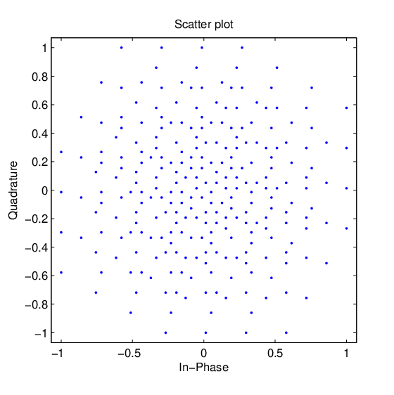
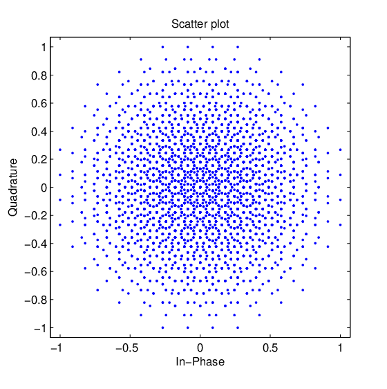
In Fig. 5, we plot the rate region of a two-user QMAC as a function of the quantizer resolution, , with User 1 using a 16-QAM input alphabet and User 2 using an optimally rotated version of the 16-QAM alphabet, as per (58), at SNR per user = 15 dB. The rate regions of GMAC (Gaussian MAC with Gaussian inputs and no output quantization) and CCMAC (Gaussian MAC with finite input and no output quantization [8]) are also plotted. From Fig. 5, we observe that with low precision ADCs ( or bits), the max. sum rate achieved with uniform receiver quantization is very poor compared to the max. sum rate of CCMAC. For instance, with a 2-bit uniform quantizer, the max. sum rate is 2.9144 bits which is just 49.5% of the max. sum rate of CCMAC (5.886 bits). To achieve a max. sum rate close to CCMAC, increased quantization resolution is required. For a fixed quantization resolution of bits, the degradation in the rate region due to a uniform quantizer compared to CCMAC is expected to be more with increasing number of users. This is because the sum constellation becomes more and more dense around the origin, as illustrated in Fig. 6. Figure 6(a) shows the two-user sum signal set with User 1 using 16-QAM with no rotation and User 2 using 16-QAM with rotation. Figure 6(b) shows the three-user sum signal set; User 1 using 16-QAM with no rotation and Users 2 and 3 using 16-QAM with and rotations, respectively. It can be seen that the scatter plot for the three-user sum signal set is clustered more around the origin than that for the two-user sum signal set.
III-C2 Motivation for a Non-uniform Quantizer
Since the symbols in the sum signal set are densely distributed around the origin, for a given quantization resolution of bits, the uniform quantizer may not be the best quantizer in terms of the achievable rate region. We highlight this point through a simple example. Let
| (63) |
As illustrated in Figure 7(a), with a -bit uniform quantizer, the receiver is unable to distinguish between the transmitted points and , since they both fall in the same quantization interval. It is expected that a quantizer which can distinguish between all possible transmitted points would have a better rate region than a quantizer which fails to do so. Hence, as shown in Fig. 7(b), with bits, a non-uniform quantizer, which distinguishes between all possible transmitted points, would have a better rate region than what is achieved by a bit uniform quantizer. In the following subsection, we propose a non-uniform quantizer for QMAC. We will see that indeed the proposed non-uniform quantizer enlarges the rate region.
III-D A Non-uniform Quantizer for QMAC
In this subsection, we propose a non-uniform quantizer for QMAC. The function for the real component of the received signal in the proposed non-uniform quantizer is
| (64) |
where , and defined in (60). Likewise, for the imaginary component
| (65) |
where and defined in (60).
Note that the parameter in (64) and (65) is a quantizer design parameter, which is used to increase/decrease the quantization granularity around the origin. It can be seen that the uniform quantizer in (61), (62) is a special case of this non-uniform quantizer with .
For a fixed rotation angle and a quantizer resolution of bits, the sum rate is a function of the parameter . Since the sum rate is a function of both and , we shall denote it by
| (66) |
For a fixed , the optimal quantizer parameter, , which maximizes the sum rate is given by
| (67) |
For a fixed , we now present a low-complexity iterative algorithm to find a suboptimum solution to the maximization problem in (67).
III-D1 An Iterative Algorithm to Solve (67)
Let and denote the value of and the sum rate in the th iteration, respectively. The algorithm starts with . In the th iteration, evaluate . If , then go to the next iteration with and . If , then evaluate (66) for all values of in the set
| (68) |
where is the search granularity of the algorithm. Find
| (69) |
Output as the solution and stop.
In the above, the algorithm iteratively increments in steps of one until the sum rate can not be further increased after some iteration . At this point, a finer granularity search is performed in the neighborhood of . It is observed numerically that monotonically increases as a function of for a fixed , and hence, with a sufficiently low value of , the value of is expected to be close to . The rotation angle that maximizes is then given by
| (70) |
III-D2 Results and Discussion
We compute the rate regions achieved by the proposed non-uniform quantizer for a two-user QMAC with User 1 using a QAM alphabet and User 2 using the optimally rotated QAM, and compare them with those achieved by the uniform quantizer. Figure 8 shows the rate regions for 64-QAM at SNR per user = 22 dB, and Fig. 9 shows the rate regions for 16-QAM at SNR per user = 15 dB. From Fig. 8, we observe that the maximum achievable sum rate with a -bit uniform quantizer is 3.0891 bits, whereas a -bit non-uniform quantizer achieves a max. sum rate of 3.7486 bits, which is a increase in the max. sum rate. This shows that significant enlargement in the rate region is achieved with non-uniform quantization compared to uniform quantization. Table II presents a summary of the observations from Figs. 8 and 9.
| Uniform | Non-uniform | |||
| # quant. | Quantizer | Quantizer | % gain | |
| bits, | ||||
| (bits) | (bits) | |||
| User 1: 16-QAM, User 2: Optimally rotated 16-QAM (Fig. 9) | ||||
| 2.9144 | 3.4675 | 2.9 | 18.98 | |
| 4.6290 | 5.0787 | 1.3 | 09.71 | |
| User 1: 64-QAM, User 2: Optimally rotated 64-QAM (Fig. 8) | ||||
| 3.0891 | 3.7486 | 3.2 | 21.35 | |
| 4.8910 | 5.1790 | 1.6 | 05.89 | |
IV Conclusions
We studied the achievable rate region of quantized broadcast and MAC channels. We showed that the capacity region expressions known for a GBC can not be used as such for QBC as the channel is no more degraded. We proposed a new achievable rate region for two-user QBC based on two different schemes. We studied the proposed achievable rate region of two-user QBC when both the users employ uniform receiver quantization. We studied the effect of rotating one of the user’s input alphabet on the proposed achievable rate region of QBC. Further, we investigated the effect of receiver quantization on the achievable rate region of QMAC. Low-precision quantization was shown to significantly degrade the rate region. Uniform quantization was found to result in significant rate loss due to the dense distribution of the sum signal set near the origin. We proposed a non-uniform quantizer that achieved significant enlargement of the achievable rate region compared to that with a uniform quantizer.
References
- [1] R. H. Walden, ADC Survey and Analysis, IEEE Jl. Sel. Areas in Commun., vol. 17, no. 4, pp. 539-550, April 1999.
- [2] G. Middleton and A. Sabharwal, “On the impact of finite receiver resolution in fading channels,” Allerton Conf. on Communication, Control and Computing, September 2006.
- [3] A. Mezghani, M. S. Khoufi, and J. A. Nossek, “Maximum likelihood detection for quantized MIMO systems,” The Intl. Workshop on Smart Antennas (WSA’2008), pp. 278-284, Darmstadt, February 2008.
- [4] J. Singh, O. Dabeer, and U. Madhow, “On the limits of communication with low-precision analog-to-digital conversion at the receiver,” IEEE Tran. Commun., vol. 52, no. 12, pp. 3629-3639, December 2009.
- [5] Gamal, A.E., “The capacity of a class of broadcast channels,” IEEE Trans. Inform. Theory, vol. 25, pp. 166-169, March 1979.
- [6] N. Deshpande and B. Sundar Rajan, “Constellation constrained capacity of two-user broadcast channels,” Proc. IEEE GLOBECOM’09, Honolulu, November-December 2009.
- [7] E. Biglieri, Coding for wireless channels, Springer-Verlag, NY, 2005.
- [8] J. Harshan and B. Sundar Rajan, “Finite signal-set capacity of two-user Gaussian multiple access channel,” Proc. IEEE ISIT’2008, pp. 1203-1207, July 2008.
- [9] T. M. Cover and J. A. Thomas, Elements of Information Theory, 2nd Edition, Wiley Series in Telecommmun. and Sig. Proc., 1999.
- [10] T. M. Cover, “Broadcast channels,” IEEE Trans. Inform. Theory, vol. IT-18, no. 1, pp. 2-14, January 1972.
- [11] S. Boyd and L. Vandenberghe, Convex Optimization, Cambridge University Press, 2004.
- [12] Suresh Chandrasekaran, Saif K. Mohammed, and A. Chockalingam, “On the capacity of quantized Gaussian MAC channels with finite input alphabet,” to appear in Proc. IEEE ICC’2011, Kyoto, June 2011.