Light-cone Gauge String Field Theory
and Dimensional Regularization

Nobuyuki Ishibashi^1, and Koichi Murakami^2, Note: e-mail: ishibash@het.ph.tsukuba.ac.jp Note: e-mail: koichimurakami71@gmail.com

Abstract

We review our recent proposals to dimensionally regularize the light-cone gauge string field theory.

1 Introduction

One of the biggest problems in string field theory is how to treat the contact term divergences [1, 2, 3, 4, 5]. There are several proposals to do so for Witten’s open string field theory [6, 7, 8]. We have shown that the dimensional regularization can be employed to deal with it [9, 10, 11, 12, 13] in the case of the light-cone gauge string field theory. It is possible to formulate the light-cone gauge string field theory in noncritical spacetime dimension $d$ . We can define scattering amplitudes as analytic functions of $d$ and obtain those in the critical dimensions by taking the limit $d\to 10$ . In this note, we would like to outline the procedure, focusing on points which were not discussed explicitly in the original references.

2 Light-cone gauge SFT

Let us start by recapitulating how to define the light-cone gauge string field theory in critical dimensions.

2.1 Light-cone gauge SFT action

Light-cone gauge string field theory for closed bosonic strings can be described by the action [14, 15]

\displaystyle S

\displaystyle=

\displaystyle\int\left[\frac{1}{2}\Phi\cdot K\Phi+\frac{g}{6}\Phi\cdot\left(\Phi\ast\Phi\right)\right]\ .

(1)

Here the string field $\Phi$ is an element of the Hilbert space of the transverse variables $X^{i}$ which satisfies the level matching condition:

	$\displaystyle\left\|\Phi\left(t,\alpha\right)\right\rangle$	$\displaystyle\in$	$\displaystyle\mathcal{H}_{X^{i}}\ \left(i=1,\cdots,d-2=24\right)\ ,$
			$\displaystyle\left(L_{0}-\tilde{L}_{0}\right)\left\|\Phi\left(t,\alpha\right)\right\rangle=0\ .$

It is a function of $t\equiv x^{+},\alpha=2p^{+}$ . The inner product of the string fields is defined as

\displaystyle\int\Phi_{1}\cdot\Phi_{2}

\displaystyle\equiv

\displaystyle\int dt\frac{\alpha d\alpha}{4\pi}\left\langle\Phi_{1}\left(t,-\alpha\right)|\Phi_{2}\left(t,\alpha\right)\right\rangle\ .

The kinetic operator $K$ is given as

\displaystyle K

\displaystyle\equiv

\displaystyle i\partial_{t}-\frac{L_{0}+\tilde{L}_{0}-\frac{d-2}{12}}{\alpha}\ .

Refer to caption — Figure 1: Three string vertex for $\alpha_{1},\alpha_{2}>0,\,\alpha_{3}<0$

The action includes only a three string interaction term. The interaction term can be defined by using the state-operator correspondence. To a string field $\left|\Phi\right\rangle$ , there corresponds a local operator $\mathcal{O}_{\Phi}(z)$ such that

\displaystyle\left|\Phi\right\rangle

\displaystyle=

\displaystyle\mathcal{O}_{\Phi}(0)\left|0\right\rangle\ ,

where $\left|0\right\rangle$ is the SL( $2,\mathbb{C}$ ) invariant vacuum. Then the integral for three string fields can be given as

	$\displaystyle\int\Phi_{1}\cdot\left(\Phi_{2}\ast\Phi_{3}\right)$	$\displaystyle=$	$\displaystyle\int dt\prod_{r=1}^{3}\left(\frac{\alpha_{r}d\alpha_{r}}{4\pi}\right)\delta\left(\sum_{r=1}^{3}\alpha_{r}\right)$		(2)
			$\displaystyle\hphantom{\int dt}\times\left\langle h_{1}\circ\mathcal{O}_{\Phi_{1}\left(t,\alpha_{1}\right)}h_{2}\circ\mathcal{O}_{\Phi_{2}\left(t,\alpha_{2}\right)}h_{3}\circ\mathcal{O}_{\Phi_{3}\left(t,\alpha_{3}\right)}\right\rangle_{\Sigma}\ ,$		(2)

where $h_{r}\,\left(r=1,2,3\right)$ are the maps which are depicted in Fig. 1.

The worldsheet theory for the light-cone gauge SFT possesses nonvanishing Virasoro central charge even in the critical case. This fact makes the calculation of the correlation function on the right hand side of eq.(2) a little bit complicated. It can be evaluated by using the Mandelstam mapping [16]

\displaystyle\rho\left(z\right)

\displaystyle=

\displaystyle\sum_{r=1}^{3}\alpha_{r}\ln\left(z-Z_{r}\right)\ ,

which maps the complex plane to $\Sigma$ as is described in Fig. 2. Using this, we can rewrite the correlation functions in terms of those on the complex plane. Because of the conformal anomaly, we obtain

	$\displaystyle\left\langle h_{1}\circ\mathcal{O}_{\Phi_{1}}h_{2}\circ\mathcal{O}_{\Phi_{2}}h_{3}\circ\mathcal{O}_{\Phi_{3}}\right\rangle_{\Sigma}$
	$\displaystyle\quad=\left\langle\left(\rho^{-1}h_{1}\right)\circ\mathcal{O}_{\Phi_{1}}\left(\rho^{-1}h_{2}\right)\circ\mathcal{O}_{\Phi_{2}}\left(\rho^{-1}h_{3}\right)\circ\mathcal{O}_{\Phi_{3}}\right\rangle_{\mathbb{C}}e^{-\Gamma\left[\ln\left(\partial\rho\bar{\partial}\bar{\rho}\right)\right]}\ ,$

where

\displaystyle\Gamma\left[\phi\right]

\displaystyle=

\displaystyle-\frac{1}{\pi}\int d^{2}z\partial\phi\bar{\partial}\phi

(3)

is the Liouville action. Using this form, the right hand side of eq.(2) is given as

	$\displaystyle\int\Phi_{1}\cdot\left(\Phi_{2}\ast\Phi_{3}\right)$
	$\displaystyle\quad=\int dt\prod_{r=1}^{3}\left(\frac{\alpha_{r}d\alpha_{r}}{4\pi}\right)\delta\left(\sum_{r=1}^{3}\alpha_{r}\right)$
	$\displaystyle\hphantom{\quad=\int\prod_{r=1}^{3}}\times\left\langle\left(\rho^{-1}h_{1}\right)\circ\mathcal{O}_{\Phi_{1}}\left(\rho^{-1}h_{2}\right)\circ\mathcal{O}_{\Phi_{2}}\left(\rho^{-1}h_{3}\right)\circ\mathcal{O}_{\Phi_{3}}\right\rangle_{\mathbb{C}}$
	$\displaystyle\hphantom{\quad=\int\prod_{r=1}^{3}}\times e^{-\Gamma\left[\ln\left(\partial\rho\bar{\partial}\bar{\rho}\right)\right]}\ .$

The Liouville action $\Gamma\left[\ln\left(\partial\rho\bar{\partial}\bar{\rho}\right)\right]$ for the Mandelstam mapping can be calculated by using the method explained later. In this case, we obtain

	$\displaystyle e^{-\Gamma\left[\ln\left(\partial\rho\bar{\partial}\bar{\rho}\right)\right]}$	$\displaystyle=$	$\displaystyle\frac{\exp\left(-2\sum_{r}\frac{\hat{\tau}_{0}}{\alpha_{r}}\right)}{\alpha_{1}\alpha_{2}\alpha_{3}}\ ,$		(4)
	$\displaystyle\hat{\tau}_{0}$	$\displaystyle\equiv$	$\displaystyle\sum_{r=1}^{3}\alpha_{r}\ln\left\|\alpha_{r}\right\|\ .$

Therefore the three string vertex in the light-cone gauge consists of LPP part and the part which comes from the anomaly.

2.2 Amplitudes

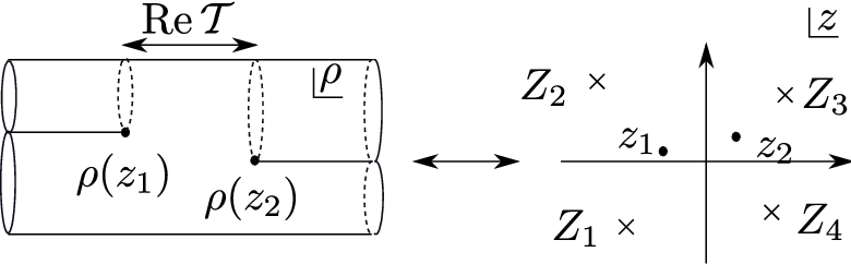
Amplitudes in the light-cone gauge SFT can be evaluated by using the propagator and the vertex derived form the action (1). The tree level four string amplitudes correspond to the Feynman diagram depicted in Fig. 3. We can evaluate tree level $N$ string amplitudes by mapping the worldsheet to the complex plane by the Mandelstam mapping

\displaystyle\rho\left(z\right)

\displaystyle=

\displaystyle\sum_{r=1}^{N}\alpha_{r}\ln\left(z-Z_{r}\right)\ .

(5)

As in the three string vertex, the amplitudes can be written in terms of the correlation functions on the complex plane as

\displaystyle\mathcal{A}_{N}

\displaystyle=

\displaystyle\sum_{\mathrm{channels}}\int\prod_{\mathcal{I}}d^{2}\mathcal{T}_{\mathcal{I}}\left\langle\prod_{r}V_{r}^{\mathrm{LC}}\right\rangle_{\mathbb{C}}e^{-\Gamma\left[\ln\partial\rho\bar{\partial}\bar{\rho}\right]}\ .

(6)

Here $V_{r}^{\mathrm{LC}}$ is the vertex operator corresponding to the $r$ -th external line, whose explicit form is given in Ref. \citenBaba:2009ns. $e^{-\Gamma\left[\ln\partial\rho\bar{\partial}\bar{\rho}\right]}$ is the factor coming from the conformal anomaly.

2.3 Evaluation of $-\Gamma$

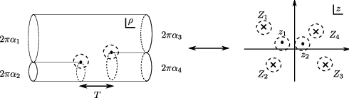
In principle, $-\Gamma$ can be calculated by substituting (5) into (3). However, $\partial\phi$ diverges at $z=Z_{r},\,z_{I}$ , where $z_{I}\,\left(I=1,\cdots,N-2\right)$ are the coordinates of the interaction points on the complex plane. In order to get a meaningful result, we need to regularize the divergences. A method to perform such calculations were given by Mandelstam [17]. Here we briefly review his method. An alternative way to evaluate $-\Gamma$ is given in Appendix C of Ref. \citenBaba:2009ns.

In order to regularize the divergences, we consider the complex plane with small discs around $z=Z_{r},z_{I},\infty$ with radii $\epsilon_{r},\epsilon_{I},\epsilon_{\infty}$ excised as shown in Fig. 4 and evaluate the Liouville action on this surface with boundaries. $-\Gamma$ diverges in the limit $\epsilon_{r},\epsilon_{I},\epsilon_{\infty}\to 0$ . We would like to calculate $-\Gamma$ keeping the reparametrization invariance and add reparametrization invariant and local counterterms to make it finite.

$-\Gamma$ can be given as a sum of the contributions from the boundaries. The Liouville action for $\phi$ on the surface can be expressed as a sum over surface terms. With discs excised, the Liouville action for the flat metric is given as a function of $\epsilon_{r},\epsilon_{I},\epsilon_{\infty}$ . Since these cutoff parameters are not reparametrization invariant as we will see, we should add the flat metric contribution to keep the reparametrization invariance.

For example, let us consider the disc around $z=Z_{r}$ . Excising a disc of radius $\epsilon_{r}\ll 1$ around $z=Z_{r}$ corresponds to making the external cylinder of the $r$ -th external line to be of the length $\alpha_{r}T_{r}\gg 1$ . $T_{r}$ is invariant under the reparametrization because $\rho$ is transformed as a scalar. The relation between $\epsilon_{r}$ and $T_{r}$ is given as

	$\displaystyle\epsilon_{r}$	$\displaystyle\sim$	$\displaystyle e^{-T_{r}+\mathrm{Re}\bar{N}_{00}^{rr}}\ ,$
	$\displaystyle\bar{N}_{00}^{rr}$	$\displaystyle\equiv$	$\displaystyle\frac{\rho\left(z_{I^{\left(r\right)}}\right)}{\alpha_{r}}-\sum_{s\neq r}\frac{\alpha_{s}}{\alpha_{r}}\ln\left(Z_{r}-Z_{s}\right)\ .$		(7)

Here $z_{I^{\left(r\right)}}$ denotes the interaction point where the $r$ -th external line interacts. The contribution to the Liouville action for $\phi$ is given as

-2\ln\left|\alpha_{r}\right|+2\ln\epsilon_{r}\ ,

and that to the Liouville action for the flat metric is

-4\ln\epsilon_{r}\ .

Therefore the contribution of this boundary to $e^{-\Gamma}$ is given as

\frac{e^{-2\mathrm{Re}\bar{N}_{00}^{rr}}}{\left|\alpha_{r}\right|^{2}}e^{2T_{r}}\ .

Other boundaries can be treated in the same way. The disc of radius $\epsilon_{I}\ll 1$ around $z=z_{I}$ on the complex plane corresponds to a disc of radius $r_{I}$ on the $\rho$ plane and

\displaystyle r_{I}

\displaystyle\sim

\displaystyle\frac{1}{2}\left|\partial^{2}\rho\left(z_{I}\right)\right|\epsilon_{I}^{2}\ .

The contribution to $e^{-\Gamma}$ is given as

\frac{1}{\left|\partial^{2}\rho\left(z_{I}\right)\right|\left(2r_{I}\right)^{5}}\ .

The disc of radius $\epsilon_{\infty}\ll 1$ around $z=\infty$ on the complex plane corresponds to a disc of radius $r_{\infty}$ on the $\rho$ plane and

\displaystyle r_{\infty}

\displaystyle\sim

\displaystyle\left|\sum_{r}\alpha_{r}Z_{r}\right|\epsilon_{\infty}\ .

The contribution to $e^{-\Gamma}$ is given as

\left|\sum_{r}\alpha_{r}Z_{r}\right|^{4}r_{\infty}^{-4}\ .

$r_{I},r_{\infty}$ are the reparametrization invariant cutoff parameters. Putting all these together, we get

\displaystyle e^{-\Gamma}

\displaystyle\sim

\displaystyle\frac{\left|\sum_{s}\alpha_{s}Z_{s}\right|^{4}e^{-2\sum_{r}\mathrm{Re}\bar{N}_{00}^{rr}}}{\prod_{r}\left|\alpha_{r}\right|^{2}\prod_{I}\left|\partial^{2}\rho\left(z_{I}\right)\right|}\cdot r_{\infty}^{-4}\prod_{r}e^{2T_{r}}\prod_{I}\left(2r_{I}\right)^{-5}\ .

Divergent factor $r_{\infty}^{-4}\prod_{r}e^{2T_{r}}\prod_{I}\left(2r_{I}\right)^{-5}$ can be absorbed into the normalizations of the coupling constant $g$ and the wave functions of the external lines. Thus we get the following form of $e^{-\Gamma}$ :

\displaystyle e^{-\Gamma\left[\ln\left(\partial\rho\bar{\partial}\bar{\rho}\right)\right]}

\displaystyle=

\displaystyle\frac{\left|\sum_{s}\alpha_{s}Z_{s}\right|^{4}e^{-2\sum_{r}\mathrm{Re}\bar{N}_{00}^{rr}}}{\prod_{r}\left|\alpha_{r}\right|^{2}\prod_{I}\left|\partial^{2}\rho\left(z_{I}\right)\right|}\ .

(8)

For $N=3$ , the right hand side coincides with eq.(4). The normalization for general $N$ can be fixed by examining the factorization properties [9].

The right hand side of eq.(6) can be turned into an integral over the moduli space. With the form of $-\Gamma$ given in (8), one can show that the amplitudes given in eq.(6) coincide with the usual first-quantized results [10].

3 Light-cone gauge SFT in noncritical dimensions

There is no problem in defining the light-cone gauge SFT for $d\neq 26$ . We write down the action

\displaystyle S

\displaystyle=

\displaystyle\int\left[\frac{1}{2}\Phi\cdot K\Phi+\frac{g}{6}\Phi\cdot\left(\Phi\ast\Phi\right)\right]\ ,

where this time

\displaystyle K

\displaystyle\equiv

\displaystyle i\partial_{t}-\frac{L_{0}+\tilde{L}_{0}-\frac{d-2}{12}}{\alpha}\ ,

and

	$\displaystyle\int\Phi_{1}\cdot\left(\Phi_{2}\ast\Phi_{3}\right)$
	$\displaystyle\quad=\int dt\prod_{r=1}^{3}\left(\frac{\alpha_{r}d\alpha_{r}}{4\pi}\right)\delta\left(\sum_{r=1}^{3}\alpha_{r}\right)$
	$\displaystyle\hphantom{\quad=\int\prod_{r=1}^{3}}\times\left\langle\left(\rho^{-1}h_{1}\right)\circ\mathcal{O}_{\Phi_{1}}\left(\rho^{-1}h_{2}\right)\circ\mathcal{O}_{\Phi_{2}}\left(\rho^{-1}h_{3}\right)\circ\mathcal{O}_{\Phi_{3}}\right\rangle_{\mathbb{C}}$
	$\displaystyle\hphantom{\quad=\int\prod_{r=1}^{3}}\times e^{-\frac{d-2}{24}\Gamma\left[\ln\left(\partial\rho\bar{\partial}\bar{\rho}\right)\right]}\ .$

The amplitudes are calculated in the same way as those in the critical case:

\displaystyle\mathcal{A}_{N}

\displaystyle=

\displaystyle\sum_{\mathrm{channels}}\int\prod_{\mathcal{I}}d^{2}\mathcal{T}_{\mathcal{I}}\left\langle\prod_{r}V_{r}^{\mathrm{LC}}\right\rangle_{\mathbb{C}}e^{-\frac{d-2}{24}\Gamma\left[\ln\left(\partial\rho\bar{\partial}\bar{\rho}\right)\right]}\ .

(9)

We would like to turn the form of the amplitude in eq.(9) into an integral over the moduli space. The moduli parameters can be taken to be the positions of the vertex operators on the complex plane. In doing so, there are two points to be checked.

One thing is the SL( $2,\mathbb{C}$ ) invariance. The integrand on the right hand side is given in terms of the quantities defined on the complex plane, but it was originally defined on the $\rho$ plane. Therefore we expect that we eventually obtain an SL( $2,\mathbb{C}$ ) invariant expression. Indeed it is easy to check the invariance.¹¹ 1 The one-loop amplitudes can be shown to be invariant under the modular transformation [18].

Another thing to be checked is if the contributions from various channels are smoothly connected. In string field theory, the amplitudes are given as a sum over contributions from various channels. Each channel corresponds to a region in the moduli space. We need to check if the integrand is smoothly connected at the boundaries of these regions as indicated in Fig. 5 so that the $\mathcal{A}_{N}$ is given as an integral of a smooth function over the moduli space. If the integrand is discontinuous at the boundaries, we have troubles in proving various symmetries of the amplitudes. It is easy to check that there are no discontinuities and we obtain an integral of a smooth function over the moduli space.

Thus the amplitudes for the noncritical string field theory can be constructed without any trouble. Therefore it seems that there is nothing wrong in considering the string field theory in noncritical dimensions.

4 Contact term divergences and dimensional regularization

The noncritical string field theory can be used to regularize the contact term divergences. It is possible to define light-cone gauge superstring field theory in noncritical dimensions as in the bosonic case. Taking $d\neq 10$ naively, we obtain a theory with only spacetime bosons which cannot be used to regularize the amplitudes with spacetime fermions. In order to deal with fermions, we need to modify the worldsheet theory. Details of such a treatment will be given elsewhere.

The amplitudes can be given as

\mathcal{A}_{N}=\sum_{\mathrm{channels}}\int\prod_{\mathcal{I}}d^{2}\mathcal{T}_{\mathcal{I}}\left\langle\prod_{I}\left|\left(\partial^{2}\rho\right)^{-\frac{3}{4}}T_{F}\left(z_{I}\right)\right|^{2}\prod_{r}V_{r}^{\mathrm{LC}}\right\rangle_{\mathbb{C}}e^{-\frac{d-2}{16}\Gamma\left[\ln\left(\partial\rho\bar{\partial}\bar{\rho}\right)\right]}\ .

(10)

Compared with the bosonic case (9), the big difference is the existence of the transverse supercurrent $T_{F}$ at the interaction points. When some interaction points come close to each other, the correlation function diverges for $d=10$ and we cannot define $\mathcal{A}_{N}$ even for tree amplitudes. However, it can be shown that for $\left|z_{I}-z_{J}\right|\sim 0$ ,

e^{-\frac{d-2}{16}\Gamma\left[\ln\left(\partial\rho\bar{\partial}\bar{\rho}\right)\right]}\sim\left|z_{I}-z_{J}\right|^{-\frac{d-2}{8}}\ ,

and taking $d$ largely negative we can make $\mathcal{A}_{N}$ well-defined. We can define $\mathcal{A}_{N}$ as an analytic function of $d$ and take the limit $d\to 10$ . If the limit is finite, a definition of $\mathcal{A}_{N}$ for $d=10$ can be obtained. If the limit is divergent, we should add counterterms to make it finite.

5 Conformal gauge formulation

One can show that the tree amplitudes defined by the dimensional regularization are finite in the limit $d\to 10$ and reproduce the results of the first-quantized formalism. This fact can be shown by constructing the conformal gauge formulation of the noncritical strings.

In the conformal gauge, the noncritical light-cone gauge strings should correspond to a worldsheet theory in a Lorentz noninvariant background. The conformal gauge formulation can be constructed by the following reasonings. The light-cone gauge worldsheet theory can be described by the path integral

\int\left[dX^{i}\right]e^{-S^{\mathrm{LC}}}\ ,

(11)

where

S^{\mathrm{LC}}=\frac{1}{2\pi}\int d^{2}z\partial X^{i}\bar{\partial}X^{i}

is the worldsheet action for the transverse variables $X^{i}\,\left(i=1,\cdots,d-2\right)$ . This action can be considered as the gauge fixed version of the standard Nambu-Goto action $S^{\mathrm{NG}}$ and the path integral should correspond to

\int\left[dX^{\mu}\right]e^{-S^{\mathrm{NG}}}\ .

(12)

For $d\neq 26$ , we need to specify the worldsheet metric which should be used to define the path integral measure $\left[dX^{\mu}\right]$ . In the light-cone gauge, the natural metric on the worldsheet is

	$\displaystyle ds^{2}$	$\displaystyle=$	$\displaystyle d\rho d\bar{\rho}$
		$\displaystyle\sim$	$\displaystyle\partial X^{+}\bar{\partial}X^{+}dzd\bar{z}\ .$

Therefore the path integral (12) should be written as

\int\left[dX^{\mu}\right]_{\partial X^{+}\bar{\partial}X^{+}}e^{-S^{\mathrm{NG}}}\ ,

(13)

where we have indicated the metric $\partial X^{+}\bar{\partial}X^{+}$ to be used to define the measure. In the conformal gauge, eq.(13) corresponds to the action

\frac{1}{2\pi}\int d^{2}z\partial X^{\mu}\bar{\partial}X_{\mu}+\frac{d-26}{24}\Gamma\left[\partial X^{+}\bar{\partial}X^{+}\right]\ .

For $d\neq 26$ , this worldsheet theory is not Lorentz invariant.

The longitudinal part of the worldsheet theory defines a nontrivial CFT. One can derive the energy-momentum tensor as

\displaystyle T\left(z\right)

\displaystyle\equiv

\displaystyle\partial X^{+}\partial X^{-}-\frac{d-26}{12}\left\{X^{+},z\right\}\ ,

(14)

where

\displaystyle\left\{X^{+},z\right\}

\displaystyle\equiv

\displaystyle\frac{\partial^{3}X^{+}}{\partial X^{+}}-\frac{3}{2}\left(\frac{\partial^{2}X^{+}}{\partial X^{+}}\right)^{2}

is the Schwarzian derivative. Such a conformal field theory can be analyzed by using the path integral formalism [10]. One can show that the energy-momentum tensor (14) satisfies the Virasoro algebra with $c=28-d$ . Therefore, with the transverse part and the reparametrization ghosts, the worldsheet theory is with nilpotent BRST charge.

We can construct the BRST invariant conformal gauge formulation in a similar way for superstrings. When all the external lines are bosonic, one can rewrite the light-cone gauge amplitudes (10) into a BRST invariant form in the conformal gauge formulation. Using such a form, it is possible to show that the dimensionally regularized tree amplitudes has a finite $d\to 10$ limit and the results coincide with those of the first-quantized formalism [18, 13].

6 Summary

We have shown that the dimensional regularization is a useful tool to deal with the contact term divergences of light-cone gauge string field theory. Our method would be applicable to the gauge invariant SFT’s [19, 20] with joining-splitting type interactions. Moreover the conformal gauge formulation in section 5 may shed light on the construction of covariant SFT of this type [21, 22].

Acknowledgements

We would like to thank the organizers of the conference for a wonderful meeting where many exciting developments are presented and discussed. This work was supported in part by Grant-in-Aid for Scientific Research (C) (20540247) from the Ministry of Education, Culture, Sports, Science and Technology (MEXT) of Japan.

References

[1] J. Greensite and F. R. Klinkhamer, “NEW INTERACTIONS FOR SUPERSTRINGS,” \NPB281,1987,269.
[2] J. Greensite and F. R. Klinkhamer, “SUPERSTRING AMPLITUDES AND CONTACT INTERACTIONS,” \NPB304,1988,108.
[3] J. Greensite and F. R. Klinkhamer, “CONTACT INTERACTIONS IN CLOSED SUPERSTRING FIELD THEORY,” \NPB291,1987,557.
[4] M. B. Green and N. Seiberg, “CONTACT INTERACTIONS IN SUPERSTRING THEORY,” \NPB299,1988,559.
[5] C. Wendt, “SCATTERING AMPLITUDES AND CONTACT INTERACTIONS IN WITTEN’S SUPERSTRING FIELD THEORY,” \NPB314,1989,209.
[6] I. Y. Arefeva, P. B. Medvedev, and A. P. Zubarev, “NEW REPRESENTATION FOR STRING FIELD SOLVES THE CONSISTENCY PROBLEM FOR OPEN SUPERSTRING FIELD THEORY,” \NPB341,1990,464.
[7] C. R. Preitschopf, C. B. Thorn, and S. A. Yost, “SUPERSTRING FIELD THEORY,” \NPB337,1990,363.
[8] N. Berkovits, “SuperPoincare invariant superstring field theory,” \NPB450,1995,90, arXiv:hep-th/9503099.
[9] Y. Baba, N. Ishibashi, and K. Murakami, “Light-Cone Gauge Superstring Field Theory and Dimensional Regularization,” \JHEP10,2009,035, arXiv:0906.3577 [hep-th].
[10] Y. Baba, N. Ishibashi, and K. Murakami, “Light-Cone Gauge String Field Theory in Noncritical Dimensions,” \JHEP12,2009,010, arXiv:0909.4675 [hep-th].
[11] Y. Baba, N. Ishibashi, and K. Murakami, “Light-cone Gauge NSR Strings in Noncritical Dimensions,” \JHEP01,1010,119, arXiv:0911.3704 [hep-th].
[12] Y. Baba, N. Ishibashi, and K. Murakami, “Light-cone Gauge Superstring Field Theory and Dimensional Regularization II,” \JHEP08,2010,102, arXiv:0912.4811 [hep-th].
[13] N. Ishibashi and K. Murakami, “Light-cone Gauge NSR Strings in Noncritical Dimensions II – Ramond Sector,” \JHEP01,2011,008, arXiv:1011.0112 [hep-th].
[14] M. Kaku and K. Kikkawa, “The Field Theory of Relativistic Strings, Pt. 1. Trees,” \PRD10,1974,1110.
[15] M. Kaku and K. Kikkawa, “The Field Theory of Relativistic Strings. 2. Loops and Pomerons,” \PRD10,1974,1823.
[16] S. Mandelstam, “Interacting String Picture of Dual Resonance Models,” \NPB64,1973,205.
[17] S. Mandelstam, “THE INTERACTING STRING PICTURE AND FUNCTIONAL INTEGRATION,”. Lectures given at Workshop on Unified String Theories, Santa Barbara, CA, Jul 29 - Aug 16, 1985.
[18] K. Murakami and N. Ishibashi, “Amplitudes in noncritical dimensions and dimensional regularization.” in this volume.
[19] H. Hata, K. Itoh, T. Kugo, H. Kunitomo, and K. Ogawa, “Covariant String Field Theory,” \PRD34,1986,2360.
[20] H. Hata, K. Itoh, T. Kugo, H. Kunitomo, and K. Ogawa, “Covariant String Field Theory. 2,” \PRD35,1987,1318.
[21] H. Hata, K. Itoh, T. Kugo, H. Kunitomo, and K. Ogawa, “BRS INVARIANT VERTEX OF NEVEU-SCHWARZ-RAMOND SUPERSTRING,” \PTP78,1987,453.
[22] T. Kugo and B. Zwiebach, “Target space duality as a symmetry of string field theory,” \PTP87,1992,801, arXiv:hep-th/9201040.

Light-cone Gauge String Field Theory and Dimensional Regularization

Abstract

1 Introduction

2 Light-cone gauge SFT

2.1 Light-cone gauge SFT action

2.2 Amplitudes

2.3 Evaluation of −Γ-\Gamma

3 Light-cone gauge SFT in noncritical dimensions

4 Contact term divergences and dimensional regularization

5 Conformal gauge formulation

6 Summary

Acknowledgements

References

Light-cone Gauge String Field Theory
and Dimensional Regularization

2.3 Evaluation of $-\Gamma$