Classical communication over a quantum interference channel

Omar Fawzi Patrick Hayden Ivan Savov Pranab Sen Mark M. Wilde ^†^†thanks: Omar Fawzi, Patrick Hayden, Ivan Savov, and Mark M. Wilde are with the School of Computer Science, McGill University, Montréal, Québec, Canada H3A 2A7. Pranab Sen is with the School of Technology and Computer Science, Tata Institute of Fundamental Research, Mumbai, India. Patrick Hayden was a visitor with the Perimeter Institute for Theoretical Physics, Waterloo, Ontario, Canada while conducting this research, and Pranab Sen was a visitor with the School of Computer Science, McGill University. This paper was presented in part at the Forty-Ninth Annual Allerton Conference, Sept.˜28-30, 2011 and the 2012 Quantum Information Processing Conference, Dec.˜12-16, 2011.

Abstract

Calculating the capacity of interference channels is a notorious open problem in classical information theory. Such channels have two senders and two receivers, and each sender would like to communicate with a partner receiver. The capacity of such channels is known exactly in the settings of “very strong” and “strong” interference, while the Han-Kobayashi coding strategy gives the best known achievable rate region in the general case.

Here, we introduce and study the quantum interference channel, a natural generalization of the interference channel to the setting of quantum information theory. We restrict ourselves for the most part to channels with two classical inputs and two quantum outputs in order to simplify the presentation of our results (though generalizations of our results to channels with quantum inputs are straightforward). We are able to determine the exact classical capacity of this channel in the settings of “very strong” and “strong” interference, by exploiting Winter’s successive decoding strategy and a novel two-sender quantum simultaneous decoder, respectively. We provide a proof that a Han-Kobayashi strategy is achievable with Holevo information rates, up to a conjecture regarding the existence of a three-sender quantum simultaneous decoder. This conjecture holds for a special class of quantum multiple access channels with average output states that commute, and we discuss some other variations of the conjecture that hold. Finally, we detail a connection between the quantum interference channel and prior work on the capacity of bipartite unitary gates.

Index Terms:

quantum Shannon theory, classical communication, quantum interference channel, quantum simultaneous decoding, quantum successive decoding, unitary gate capacity

I Introduction

Classical information theory came as a surprise to the communication engineers of the 1940s and ’50s [43, 58]. It was astonishing that two-terminal noisy communication channels generally have a non-zero capacity at which two parties can communicate error-free in the asymptotic limit of many channel uses, and furthermore, that the computation of this capacity is a straightforward convex optimization problem [53]—many consider the achievements of Shannon to be among the great scientific accomplishments of the last century. Soon after this accomplishment, Shannon laid the foundations for multi-user information theory, and he claimed that a three-terminal communication channel with two senders and one receiver also has a simple, elegant solution [54, 58]. Some time later, Liao and Ahlswede provided a formal proof of the capacity of this multiple access channel without any knowledge of Shannon’s unpublished solution [38, 2]. The beauty of information theory in these two settings is that it offers elementary solutions to problems that, at the outset, seem to be extraordinarily difficult to solve.

The situation for more general communication scenarios in multi-user information theory is not as simple and elegant as it is for single-sender, single-receiver channels and multiple access channels [17]. For example, the capacity of the interference channel is one of the notorious open problems in classical information theory [37]. The interference channel refers to the setting in which a noisy communication channel connects two senders to two receivers, and each sender’s goal is to communicate with a partner receiver. Each sender’s transmission can interfere with the other’s, and this is one reason (among many) that the problem is difficult to solve in the general case. This channel arises naturally in the context of data transmission over interfering wireless links or digital subscriber lines [37]. Shannon himself introduced the problem and attempted to solve it [54], but it is the later work of others that would provide ongoing improvements to the inner and outer bounds for the capacity of the interference channel [8, 46, 47, 48, 49, 20, 36].

Carleial offered the first surprising result for the interference channel [8], by demonstrating that each sender can achieve the same rates of communication as if there is no interference at all if the interference from the other sender’s transmission is “very strong.” Carleial’s solution is to have each receiver decode the other sender’s message first and follow by decoding the partner sender’s message, rather than each receiver simply treating the other sender’s transmission as noise. Thus, Carleial’s strategy demonstrates that we can achieve improved communication rates by taking advantage of interference rather than treating it as an obstacle. Sato then gave a full characterization of the capacity of the Gaussian interference channel in the setting of “strong” interference [49], by appealing to an earlier result of Ahlswede regarding the capacity of a compound multiple access channel [2]. Han and Kobayashi independently found Sato’s result, and they built on these insights and applied them to the most general setting (not necessarily “strong” or “very strong” interference) by allowing for each decoder to partially decode the other sender’s message and use this information to better decode the message intended for them [20]. The resulting achievable rate region is known as the Han-Kobayashi rate region, and it is currently the best known inner bound on the capacity of the interference channel.¹¹ 1 Chong, Motani, and Garg subsequently proposed another achievable rate region originally thought to improve the Han-Kobayashi rate region [9], but later work demonstrated that the Chong-Motani-Garg achievable rate region is equivalent to the Han-Kobayashi region [10, 35].

The model of the interference channel as stated in the above works is an important practical model for data transmission in a noisy two-input, two-output network, but it ignores a fundamental aspect of the physical systems employed to transmit this data. At bottom, these physical systems operate according to the laws of quantum mechanics [41], and ultimately, at some level, these laws govern how noise can affect these systems. Now, for many systems (macroscopic ones in particular), these laws are not necessary to describe the dynamics of encoding, transmission, and decoding, and one could argue in this case that there is not any benefit to recasting information theory as a quantum information theory because it would only add a layer of complexity to the theory. However, there are examples of natural physical systems, such as fiber optic cables or free space channels, for which quantum information theory offers a boost in capacity if the coding scheme makes clever use of quantum mechanics [18]. Thus, it is important to determine the information capacities of quantum channels, given that the physical carriers of information are quantum and quantum effects often give a boost in capacity. In Ref. [18], it is shown that a receiver making use of a collective measurement operating on all of the channel outputs has an improvement in performance over a receiver decoding with single-channel-output measurements. Additionally, there are existential arguments for examples of channels in which entanglement at the encoder can improve performance, leading to superadditive effects that simply cannot occur in classical information theory [25].

The quantum-mechanical approach to information theory has shed a new light on the very nature of information, and researchers have made much progress on this front in the past few decades [41]. Perhaps the most fundamental problem in quantum information theory is the task of transmitting bits over a quantum channel. Holevo and Schumacher-Westmoreland (HSW) offered independent proofs that the Holevo information, one generalization of Shannon’s mutual information, is an achievable rate for classical data transmission over a quantum channel [30, 50]. Many researchers thought for some time that the Holevo information of a quantum channel would be equal to its classical capacity, but recent work has demonstrated that the answer to the most fundamental question of the classical capacity of a quantum channel remains wide open in the general case [25, 29].

Soon after the HSW result, quantum information theorists began exploring other avenues, one of which is multi-user quantum information theory. Winter proved that the capacity region of a quantum multiple access channel is a natural generalization of the classical solution, in which we can replace Shannon information rates with Holevo information rates [62]. It was not obvious at the outset that this solution would be possible—after all, any retrieval of data from a quantum system inevitably disturbs the state of the system, suggesting that successive decoding strategies employed in the classical case might not work for quantum systems [11]. But Winter overcame this obstacle by realizing that a so-called “gentle” or “tender” measurement, a measurement with an outcome that succeeds with high probability, effectively causes no disturbance to the state in the asymptotic limit of many channel uses. Later, Yard et al. considered various capacities of a quantum broadcast channel [64], and they found results that are natural generalizations of results from classical multi-user information theory [5, 17]. In parallel with these developments, researchers have considered many generalizations of the above settings, depending on the form of the transmitted information [39, 55, 12, 28, 31, 32], whether assisting resources are available [4, 56, 33, 15], or whether the sender and receiver would like to trade off different resources against each other [14, 13, 34].

II Summary of Results

In this paper, we introduce the quantum interference channel, a natural generalization of the interference channel to the quantum domain. We at first restrict our discussion to a particular ccqq quantum interference channel, which has two classical inputs and two quantum outputs. This restriction simplifies the presentation, and a straightforward extension of our results leads to results for a general quantum interference channel with quantum inputs and quantum outputs. We summarize our main results below:

•

Our first contribution is an exact characterization of the capacity region of a ccqq quantum interference channel with “very strong” interference—the result here is a straightforward generalization of Carleial’s result from Ref. [8].
•

Our second contribution is a different exact characterization of the capacity of a ccqq channel that exhibits “strong interference.” This result employs a novel quantum simultaneous decoder for quantum multiple access channels with two classical inputs and one quantum output.
•

Our next contribution is a quantization of the Han-Kobayashi achievable rate region, up to a conjecture regarding the existence of a quantum simultaneous decoder for quantum multiple access channels with three classical inputs and one quantum output. We prove that a three-sender quantum simultaneous decoder exists in the special case where the induced channel to each receiver has average output states that commute, but we have not been able to prove the existence of such a decoder in the general case (neither is it clear how to leverage the proof of the two-sender simultaneous decoder). We prove that a certain rate region described in terms of min-entropies [45, 44] is achievable for the general non-commuting case, and our suspicion is that a proof for the most general case should exist and will bear similarities to these proofs. The existence of such a simultaneous decoder immediately implies that the senders and receivers can achieve the rates on the Han-Kobayashi inner bound. This conjecture is also closely related to the the “multiparty typicality” conjecture formulated in [16].
•

We also describe an achievable rate region for the quantum interference channel based on a successive decoding and rate splitting strategy [52].
•

We supply an outer bound on the capacity of the quantum interference channel, similar to Sato’s outer bound from Ref. [47].
•

Finally, we discuss the connection between prior work on the capacity of unitary gates [3, 22, 23, 24] and the capacity of the quantum interference channel. The quantum interference channel that we consider in this last contribution is an isometry, in which the two inputs and two outputs are quantum and the channel acts as a noiseless evolution from the senders to the receivers.

We structure this paper as follows. We first introduce the notation used in the rest of the paper. We then detail the general information processing task that two senders and two receivers are trying to accomplish using the quantum interference channel. Section V discusses the connection between the multiple access channel and the interference channel, and we prove the existence of a quantum simultaneous decoder for the multiple access channel with two classical inputs and one quantum output. This section also states a conjecture regarding the existence of a quantum simultaneous decoder with three classical inputs and one quantum output, and we prove that it exists for a special case. We also discuss an achievable rate region in terms of min-entropies, and we remark briefly on many avenues that we pursued in an attempt to prove this conjecture. Section VI presents our results regarding the quantum interference channel. We first determine the capacity of the quantum interference channel if the channel has “very strong” interference and follow with the capacity when the channel exhibits “strong” interference. We next show how to achieve the Han-Kobayashi inner bound, by exploiting the conjecture regarding the existence of a three-sender quantum simultaneous decoder. We then present a set of achievable rates obtained using successive decoding and rate splitting. This section ends with an outer bound on the capacity of the quantum interference channel. Section VII presents our final contribution regarding the connection to unitary gate capacities, and the conclusion summarizes our findings and states open lines of pursuit for the quantum interference channel.

III Notation

We denote quantum systems as $A$ , $B$ , and $C$ and their corresponding Hilbert spaces as $\mathcal{H}^{A}$ , $\mathcal{H}^{B}$ , and $\mathcal{H}^{C}$ with respective dimensions $d_{A}$ , $d_{B}$ , and $d_{C}$ . We denote pure states of the system $A$ with a ket $\left|\phi\right\rangle^{A}$ and the corresponding density operator as $\phi^{A}=\left|\phi\right\rangle\!\left\langle\phi\right|^{A}$ . All kets that are quantum states have unit norm, and all density operators are positive semi-definite with unit trace. We model our lack of access to a quantum system with the partial trace operation. That is, given a two-qubit state $\rho^{AB}$ shared between Alice and Bob, we can describe Alice’s state with the reduced density operator:

\rho^{A}=\text{Tr}_{B}\left\{\rho^{AB}\right\},

where Tr_B denotes a partial trace over Bob’s system. Let

H(A)_{\rho}\equiv-\text{Tr}\left\{\rho^{A}\log\rho^{A}\right\}

be the von Neumann entropy of the state $\rho^{A}$ . For a state $\sigma^{ABC}$ , we define the quantum conditional entropy

H(A|B)_{\sigma}\equiv H(AB)_{\sigma}-H(B)_{\sigma},

the quantum mutual information

I(A;B)_{\sigma}\equiv H(A)_{\sigma}+H(B)_{\sigma}-H(AB)_{\sigma},

and the conditional quantum mutual information

I(A;B|C)_{\sigma}\equiv H(A|C)_{\sigma}+H(B|C)_{\sigma}-H(AB|C)_{\sigma}.

Quantum operations are completely positive trace-preserving (CPTP) maps $\mathcal{N}^{A^{\prime}\rightarrow B}$ , which accept input states in $A^{\prime}$ and output states in $B$ . In order to describe the “distance” between two quantum states, we use the notion of trace distance. The trace distance between states $\sigma$ and $\rho$ is

\|\sigma-\rho\|_{1}=\mathrm{Tr}\left|\sigma-\rho\right|,

where $|X|=\sqrt{X^{\dagger}X}$ . Two states that are similar have trace distance close to zero, whereas states that are perfectly distinguishable have trace distance equal to two. Throughout this paper, logarithms and exponents are taken base two unless otherwise specified. Appendix A reviews several important properties of typical sequences and typical subspaces.

IV The Information Processing Task

We first discuss the information processing task that two senders and two receivers are trying to accomplish with the quantum interference channel. We assume that they have access to many independent uses of a particular type of channel with two classical inputs and two quantum outputs. A ccqq quantum interference channel is the following map:

x,y\rightarrow\rho_{x,y}^{B_{1}B_{2}}\text{,}

(1)

where the inputs $x$ and $y$ produce a density operator $\rho_{x,y}^{B_{1}B_{2}}$ that exists on quantum systems $B_{1}$ and $B_{2}$ . Receiver 1 has access to system $B_{1}$ , and Receiver 2 has access to system $B_{2}$ . An $\left(n,R_{1}-\delta,R_{2}-\delta,\epsilon\right)$ quantum interference channel code consists of three steps: encoding, transmission, and decoding.

Encoding. Sender 1 chooses a message $l$ from a message set $\mathcal{L}=\left\{1,2,\ldots,|\mathcal{L}|\right\}$ where $|\mathcal{L}|=2^{n(R_{1}-\delta)}$ , and Sender 2 similarly chooses a message $m$ from a message set $\mathcal{M}=\left\{1,2,\ldots,|\mathcal{M}|\right\}$ where $|\mathcal{M}|=2^{n(R_{2}-\delta)}$ , where $\delta$ is some arbitrarily small positive number. Senders 1 and 2 then encode their messages as codewords of the following form:

	$\displaystyle x^{n}\!\left(l\right)$	$\displaystyle\equiv x_{1}\!\left(l\right)\ x_{2}\!\left(l\right)\ \cdots\ x_{n}\!\left(l\right),$
	$\displaystyle y^{n}\!\left(m\right)$	$\displaystyle\equiv y_{1}\!\left(m\right)\ y_{2}\!\left(m\right)\ \cdots\ y_{n}\!\left(m\right).$

Transmission. They both input each letter of their codewords to a single use of the channel in (1), leading to an $n$ -fold tensor product state of the following form at the output:

\rho_{x^{n}\left(l\right),y^{n}\left(m\right)}^{B_{1}^{n}B_{2}^{n}}\equiv\rho_{x_{1}\left(l\right),y_{1}\left(m\right)}^{B_{1,1}B_{2,1}}\otimes\rho_{x_{2}\left(l\right),y_{2}\left(m\right)}^{B_{1,2}B_{2,2}}\otimes\cdots\otimes\rho_{x_{n}\left(l\right),y_{n}\left(m\right)}^{B_{1,n}B_{2,n}}.

Receiver 1 has access to systems $B_{1,i}$ for all $i\in\{1,\ldots,n\}$ , and Receiver 2 has access to systems $B_{2,i}$ .

Decoding. Receiver 1 performs a measurement on his systems in order to determine the message of Sender 1, and Receiver 2 similarly performs a measurement to obtain Sender 2’s message. More specifically, Receiver 1 performs a positive operator-valued measure (POVM) $\left\{\Lambda_{l}\right\}_{l\in\left\{1,\ldots,|\mathcal{L}|\right\}}$ where $\Lambda_{l}$ is a positive operator for all $l$ and $\sum_{l}\Lambda_{l}=I$ , and Receiver 2 performs a POVM $\left\{\Gamma_{m}\right\}_{m\in\left\{1,\ldots,|\mathcal{M}|\right\}}$ with similar conditions holding for the operators in this set. Figure 1 depicts all of these steps.

Refer to caption — Fig. 1: The information processing task for the quantum interference channel. Let $\mathcal{N}$ represent the quantum interference channel with two classical inputs $X$ and $Y$ and two quantum outputs $B_{1}$ and $B_{2}$ . Sender 1 selects a message $l$ to transmit (modeled by a random variable $L$ ), and Sender 2 selects a message $m$ to transmit (modeled by $M$ ). Each sender encodes their message as a codeword and transmits the codeword over many independent uses of a quantum interference channel. The receivers each receive the quantum outputs of the channel and perform a measurement to determine the message that their partner sender transmitted.

The probability of the receivers correctly decoding a particular message pair $\left(l,m\right)$ is as follows:

\Pr\left\{L^{\prime}=l,\ M^{\prime}=m\ |\ L=l,\ M=m\right\}=\\ \text{Tr}\left\{\left(\Lambda_{l}\otimes\Gamma_{m}\right)\rho_{x^{n}\left(l\right),y^{n}\left(m\right)}^{B_{1}^{n}B_{2}^{n}}\right\},

and so the probability of incorrectly decoding that message pair is

	$\displaystyle p_{e}\left(l,m\right)$	$\displaystyle\equiv\Pr\left\{(L^{\prime},M^{\prime})\neq(l,m)\ \|\ L=l,\ M=m\right\}$
		$\displaystyle=\text{Tr}\left\{\left(I-\Lambda_{l}\otimes\Gamma_{m}\right)\rho_{x^{n}\left(l\right),y^{n}\left(m\right)}^{B_{1}^{n}B_{2}^{n}}\right\},$

where $L$ and $M$ indicate random variables corresponding to the senders’ choice of messages and the primed random variables correspond to the classical outputs of the receivers’ measurements. The quantum interference channel code is $\epsilon$ -good if the average probability of error $\overline{p}_{e}$ is bounded from above by $\epsilon$ :

	$\displaystyle\overline{p}_{e}$	$\displaystyle\equiv\frac{1}{\|\mathcal{L}\|\|\mathcal{M}\|}\sum_{l,m}p_{e}\left(l,m\right)$
		$\displaystyle=\frac{1}{\|\mathcal{L}\|\|\mathcal{M}\|}\sum_{l,m}\text{Tr}\left\{\left(I-\Lambda_{l}\otimes\Gamma_{m}\right)\rho_{x^{n}\left(l\right),y^{n}\left(m\right)}^{B_{1}^{n}B_{2}^{n}}\right\}\leq\epsilon.$

A rate pair $\left(R_{1},R_{2}\right)$ is achievable if there exists an $\left(n,R_{1}-\delta,R_{2}-\delta,\epsilon\right)$ quantum interference channel code for all $\delta,\epsilon>0$ and sufficiently large $n$ . The capacity region of the quantum interference channel is the closure of the set of all achievable rates.

V Classical Communication over the Quantum Multiple Access Channel

There is a strong connection between the multiple access channel and the interference channel. In fact, inner bounds for the capacity of an interference channel can be obtained by requiring the two receivers to decode both messages. Such a strategy naturally defines two multiple access channels that share the same senders [20, 17].²² 2 The setting in which both receivers decode both messages of the two senders is the same as the setting for the compound multiple access channel [2]. It is thus important to understand two different coding approaches for obtaining the capacity of the multiple access channel.

V-A Successive Decoding

A first approach to achieve the capacity of the multiple access channel is to exploit a successive decoding strategy [11, 17], where the receiver first decodes the message of one sender while treating the other sender’s transmission as noise. The receiver then decodes the message of the other sender by exploiting the decoded information as side information. This strategy achieves one “corner point” of the capacity region, and a symmetric strategy, where the receiver decodes in the opposite order, achieves the other corner point. They can achieve any rate pair between these two corner points with a time-sharing strategy, in which they exploit successive decoding in one order for a fraction of the channel uses and they exploit successive decoding in the opposite order for the remaining fraction of the channel uses. They can achieve the other boundary points and the interior of the capacity region by resource wasting.

Winter exploited this approach for the quantum multiple access channel [62], essentially by using a random coding argument and by showing that a measurement to determine the first sender’s message causes a negligible disturbance of the channel output state. Hsieh et al. followed up on this result by showing how to perform entanglement-assisted classical communication over a quantum multiple access channel [33].

Theorem 1 (Successive Decoding [62]).

Let $x,y\rightarrow\rho_{x,y}$ be a ccq channel from two senders to a single receiver. Let $p_{X}\left(x\right)$ and $p_{Y}\left(y\right)$ be respective input distributions that each sender uses to create random codebooks of the form $\left\{X^{n}\left(l\right)\right\}_{l\in\left[1,\ldots,L\right]}$ and $\left\{Y^{n}\left(m\right)\right\}_{m\in\left[1,\ldots,M\right]}$ . Suppose that the rates $R_{1}=\frac{1}{n}\log_{2}\left(L\right)+\delta$ and $R_{2}=\frac{1}{n}\log_{2}\left(M\right)+\delta$ (where $\delta>0$ ) satisfy

	$\displaystyle R_{1}$	$\displaystyle\leq I\left(X;B\right)_{\rho},$
	$\displaystyle R_{2}$	$\displaystyle\leq I\left(Y;B\|X\right)_{\rho},$

where the Holevo information quantities are with respect to a classical-quantum state of the form

\rho^{XYB}\equiv\sum_{x,y}p_{X}\left(x\right)p_{Y}\left(y\right)\left|x\right\rangle\left\langle x\right|^{X}\otimes\left|y\right\rangle\left\langle y\right|^{Y}\otimes\rho_{x,y}^{B}.

(2)

Then there exist two POVMs $\left\{\Lambda_{l}\right\}$ and $\left\{\Gamma_{m}^{(l)}\right\}$ acting in successive order such that the expectation of the average probability of correct detection is arbitrarily close to one:

\mathbb{E}\left\{\frac{1}{LM}\sum_{l,m}\text{Tr}\left\{\sqrt{\Gamma_{m}^{(l)}}\sqrt{\Lambda_{l}}\rho_{X^{n}\left(l\right)Y^{n}\left(m\right)}\sqrt{\Lambda_{l}}\sqrt{\Gamma_{m}^{(l)}}\right\}\right\}\\ \geq 1-\epsilon,

where the expectation is with respect to $X^{n}$ and $Y^{n}$ .

V-B Quantum Simultaneous Decoding

Another approach to achieve the capacity of the multiple access channel is for the receiver to use a simultaneous decoder (sometimes referred to as a jointly typical decoder in the IID setting), which decodes the messages of all senders at the same time rather than in succession [11, 17]. On the one hand, simultaneous decoding is more complex than successive decoding because it considers all tuples of messages, but on the other hand, it is more powerful than a successive decoding strategy because it can decode at any rates provided that the rates are in the capacity region (also there is no need for time sharing).

With such a strategy and for two senders, there are four different types of errors that can occur—one of these we can bound with a standard typicality argument and the other three correspond to the bounds on the capacity region of the channel. This strategy is our approach below, and we can prove that a quantum simultaneous decoder exists for multiple access channels with two classical inputs and one quantum output. Though, for a three-sender quantum multiple access channel, we are only able to prove that a quantum simultaneous decoder exists in the special case where the averaged output states commute. Thus, we leave the general case stated as a conjecture.

V-B1 Two-Sender Quantum Simultaneous Decoding

This section contains the proof of the two-sender quantum simultaneous decoder. We should mention that Sen arrived at this result with a different technique [51].

Theorem 2 (Two-Sender Quantum Simultaneous Decoding).

$\displaystyle R_{1}$	$\displaystyle\leq I\left(X;B\|Y\right),$	(3)
$\displaystyle R_{2}$	$\displaystyle\leq I\left(Y;B\|X\right)_{\rho},$	(4)
$\displaystyle R_{1}+R_{2}$	$\displaystyle\leq I\left(XY;B\right)_{\rho},$	(5)

where the entropies are with respect to a state of the form in (2). Then there exists a simultaneous decoding POVM $\left\{\Lambda_{l,m}\right\}$ such that the expectation of the average probability of error is bounded from above by $\epsilon$ for all $\epsilon>0$ and sufficiently large $n$ .

Proof.

Suppose that the channel is a ccq channel of the form $x,y\rightarrow\rho_{x,y}$ and that the two senders have independent distributions $p_{X}\left(x\right)$ and $p_{Y}\left(y\right)$ . These distributions induce the following averaged output states:

$\displaystyle\rho_{x}$	$\displaystyle\equiv\sum_{y}p_{Y}\!\left(y\right)\rho_{x,y},$	(6)
$\displaystyle\rho_{y}$	$\displaystyle\equiv\sum_{x}p_{X}\!\left(x\right)\rho_{x,y},$	(7)
$\displaystyle\rho$	$\displaystyle\equiv\sum_{x,y}p_{X}\!\left(x\right)p_{Y}\!\left(y\right)\rho_{x,y}.$	(8)

Codeword Selection. Senders 1 and 2 choose codewords $\left\{X^{n}\left(l\right)\right\}_{l\in\left\{1,\ldots,L\right\}}$ and $\left\{Y^{n}\left(m\right)\right\}_{m\in\left\{1,\ldots,M\right\}}$ independently and randomly according to the product distributions $p_{X^{n}}\left(x^{n}\right)$ and $p_{Y^{n}}\left(y^{n}\right)$ .

POVM Construction. Let $\Pi_{\rho,\delta}^{n}$ be the typical projector for the tensor power state $\rho^{\otimes n}$ defined by (8). Let $\Pi_{\rho_{y^{n}},\delta}^{n}$ be the conditionally typical projector for the tensor product state $\rho_{y^{n}}$ defined by (7) for $n$ uses of the channel. Let $\Pi_{\rho_{x^{n}},\delta}^{n}$ be the conditionally typical projector for the tensor product state $\rho_{x^{n}}$ defined by (6) for $n$ uses of the channel. Let $\Pi_{\rho_{x^{n},y^{n}},\delta}^{n}$ be the conditionally typical projector for the tensor product state $\rho_{x^{n},y^{n}}$ defined as the output of the $n$ channels when codewords $x^{n}$ and $y^{n}$ are input. (We are using the “weak” definitions of these projectors as defined in Appendix A.) In what follows, we make the following abbreviations:

	$\displaystyle\Pi$	$\displaystyle\equiv\Pi_{\rho,\delta}^{n},$
	$\displaystyle\Pi_{y^{n}}$	$\displaystyle\equiv\Pi_{\rho_{y^{n}},\delta}^{n},$
	$\displaystyle\Pi_{x^{n}}$	$\displaystyle\equiv\Pi_{\rho_{x^{n}},\delta}^{n},$
	$\displaystyle\Pi_{x^{n},y^{n}}$	$\displaystyle\equiv\Pi_{\rho_{x^{n},y^{n}},\delta}^{n}.$

The detection POVM $\left\{\Lambda_{l,m}\right\}$ has the following form:

	$\displaystyle\Lambda_{l,m}$	$\displaystyle\equiv\left(\sum_{l^{\prime},m^{\prime}}\Pi_{l^{\prime},m^{\prime}}^{\prime}\right)^{-\frac{1}{2}}\Pi_{l,m}^{\prime}\left(\sum_{l^{\prime},m^{\prime}}\Pi_{l^{\prime},m^{\prime}}^{\prime}\right)^{-\frac{1}{2}},$		(9)
	$\displaystyle\Pi_{l,m}^{\prime}$	$\displaystyle\equiv\Pi\ \Pi_{X^{n}\left(l\right)}\ \Pi_{X^{n}\left(l\right),Y^{n}\left(m\right)}\ \Pi_{X^{n}\left(l\right)}\ \Pi.$

Observe that the operator $\Pi_{l,m}^{\prime}$ is a positive operator and thus $\left\{\Lambda_{l,m}\right\}$ is a valid POVM.

Error Analysis. The average error probability of the code has the following form:

\overline{p}_{e}\equiv\frac{1}{LM}\sum_{l,m}\text{Tr}\left\{\left(I-\Lambda_{l,m}\right)\rho_{X^{n}\left(l\right),Y^{n}\left(m\right)}\right\}.

(10)

We instead analyze the expectation of the average error probability, where the expectation is with respect to the random choice of code:

		$\displaystyle\mathbb{E}_{X^{n},Y^{n}}\left\{\overline{p}_{e}\right\}$
		$\displaystyle\equiv\mathbb{E}_{X^{n},Y^{n}}\left\{\frac{1}{LM}\sum_{l,m}\text{Tr}\left\{\left(I-\Lambda_{l,m}\right)\rho_{X^{n}\left(l\right),Y^{n}\left(m\right)}\right\}\right\}$
		$\displaystyle=\frac{1}{LM}\sum_{l,m}\mathbb{E}_{X^{n},Y^{n}}\left\{\text{Tr}\left\{\left(I-\Lambda_{l,m}\right)\rho_{X^{n}\left(l\right),Y^{n}\left(m\right)}\right\}\right\}.$

Due to the symmetry of the code construction (the fact that the expectation $\mathbb{E}_{X^{n},Y^{n}}\left\{\text{Tr}\left\{\left(I-\Lambda_{l,m}\right)\rho_{X^{n}\left(l\right),Y^{n}\left(m\right)}\right\}\right\}$ is independent of the particular message pair $\left(l,m\right)$ ), it suffices to analyze the expectation of the average error probability for the first message pair $\left(1,1\right)$ :

\mathbb{E}_{X^{n},Y^{n}}\left\{\overline{p}_{e}\right\}=\mathbb{E}_{X^{n},Y^{n}}\left\{\text{Tr}\left\{\left(I-\Lambda_{1,1}\right)\rho_{X^{n}\left(1\right),Y^{n}\left(1\right)}\right\}\right\}.

We now begin our error analysis. In what follows, we abbreviate $X^{n}$ as $X$ and $Y^{n}$ as $Y$ in order to save space. We first bound the above error probability as

		$\displaystyle\mathbb{E}_{XY}\left\{\overline{p}_{e}\right\}$
		$\displaystyle\leq\mathbb{E}_{XY}\left\{\text{Tr}\left\{\left(I-\Lambda_{1,1}\right)\ \Pi_{Y\left(1\right)}\ \rho_{X\left(1\right),Y\left(1\right)}\ \Pi_{Y\left(1\right)}\right\}\right\}$
		$\displaystyle\ \ +\mathbb{E}_{XY}\left\{\left\\|\Pi_{Y\left(1\right)}\ \rho_{X\left(1\right),Y\left(1\right)}\ \Pi_{Y\left(1\right)}-\rho_{X\left(1\right),Y\left(1\right)}\right\\|_{1}\right\}$		(11)
		$\displaystyle\leq\mathbb{E}_{XY}\left\{\text{Tr}\left\{\left(I-\Lambda_{1,1}\right)\ \Pi_{Y\left(1\right)}\ \rho_{X\left(1\right),Y\left(1\right)}\ \Pi_{Y\left(1\right)}\right\}\right\}$
		$\displaystyle\,\,\,+2\sqrt{\epsilon},$		(12)

where the first inequality follows from the inequality

\text{Tr}\left\{\Lambda\rho\right\}\leq\text{Tr}\left\{\Lambda\sigma\right\}+\left\|\rho-\sigma\right\|_{1},

(13)

which holds for all $\rho$ , $\sigma$ , and $\Lambda$ such that $0\leq\rho,\sigma,\Lambda\leq I$ . The second inequality follows from the properties of weak conditionally typical subspaces and the Gentle Operator Lemma for ensembles, by taking $n$ to be sufficiently large (a discussion of these properties is in Appendix A). The idea behind this first bound on the error probability is that we require the projector $\Pi_{Y\left(1\right)}$ in order to remove some of large eigenvalues of an averaged version of $\rho_{X\left(1\right),Y\left(1\right)}$ , and this point in the proof seems to be the most opportune time to insert it.

The Hayashi-Nagaoka operator inequality applies to a positive operator $T$ and an operator $S$ where $0\leq S\leq I$ [27, 26]:

I-\left(S+T\right)^{-\frac{1}{2}}S\left(S+T\right)^{-\frac{1}{2}}\leq 2\left(I-S\right)+4T.

Choosing

	$\displaystyle S$	$\displaystyle=\Pi_{1,1}^{\prime},$
	$\displaystyle T$	$\displaystyle=\sum_{\left(l,m\right)\neq\left(1,1\right)}\Pi_{l,m}^{\prime},$

we can apply the above operator inequality to bound the first term in (12) as

\mathbb{E}_{XY}\left\{\text{Tr}\left\{\left(I-\Lambda_{1,1}\right)\ \Pi_{Y\left(1\right)}\ \rho_{X\left(1\right),Y\left(1\right)}\ \Pi_{Y\left(1\right)}\right\}\right\}\\ \leq 2\ \mathbb{E}_{XY}\left\{\text{Tr}\left\{\left(I-\Pi_{1,1}^{\prime}\right)\ \Pi_{Y\left(1\right)}\ \rho_{X\left(1\right),Y\left(1\right)}\ \Pi_{Y\left(1\right)}\right\}\right\}\\ \qquad\ \ +4\!\!\!\!\!\!\sum_{\left(l,m\right)\neq\left(1,1\right)}\mathbb{E}_{XY}\left\{\text{Tr}\left\{\Pi_{l,m}^{\prime}\ \Pi_{Y\left(1\right)}\ \rho_{X\left(1\right),Y\left(1\right)}\ \Pi_{Y\left(1\right)}\right\}\right\}.

(14)

We first consider bounding the term in the second line above. Consider that

		$\displaystyle\mathbb{E}_{XY}\left\{\text{Tr}\left\{\Pi_{1,1}^{\prime}\ \Pi_{Y\left(1\right)}\ \rho_{X\left(1\right),Y\left(1\right)}\ \Pi_{Y\left(1\right)}\right\}\right\}$
		$\displaystyle=\mathbb{E}_{XY}\{\text{Tr}\{\Pi\ \Pi_{X\left(1\right)}\ \Pi_{X\left(1\right),Y\left(1\right)}\ \Pi_{X\left(1\right)}\ \Pi$
		$\displaystyle\ \ \ \ \ \ \ \ \ \ \ \ \ \ \ \ \ \ \ \ \ \ \ \Pi_{Y\left(1\right)}\ \rho_{X\left(1\right),Y\left(1\right)}\ \Pi_{Y\left(1\right)}\}\}$
		$\displaystyle\geq\mathbb{E}_{XY}\left\{\text{Tr}\left\{\Pi_{X\left(1\right),Y\left(1\right)}\ \rho_{X\left(1\right),Y\left(1\right)}\right\}\right\}$
		$\displaystyle\ \ \ -\mathbb{E}_{XY}\left\{\left\\|\Pi\ \rho_{X\left(1\right),Y\left(1\right)}\ \Pi-\rho_{X\left(1\right),Y\left(1\right)}\right\\|_{1}\right\}$
		$\displaystyle\ \ \ \ -\mathbb{E}_{XY}\left\{\left\\|\Pi_{Y\left(1\right)}\ \rho_{X\left(1\right),Y\left(1\right)}\ \Pi_{Y\left(1\right)}-\rho_{X\left(1\right),Y\left(1\right)}\right\\|_{1}\right\}$
		$\displaystyle\ \ \ \ \ -\mathbb{E}_{XY}\left\{\left\\|\Pi_{X\left(1\right)}\ \rho_{X\left(1\right),Y\left(1\right)}\ \Pi_{X\left(1\right)}-\rho_{X\left(1\right),Y\left(1\right)}\right\\|_{1}\right\}$
		$\displaystyle\geq 1-\epsilon-6\sqrt{\epsilon}.$		(15)

The above inequalities follow by employing the Gentle Operator Lemma for ensembles, (13), and the below inequalities that follow from the discussion in Appendix A:

$\displaystyle\mathbb{E}_{XY}\left\{\text{Tr}\{\Pi_{X\left(1\right)}\ \rho_{X\left(1\right),Y\left(1\right)}\}\right\}$	$\displaystyle\geq 1-\epsilon,$	(16)
$\displaystyle\mathbb{E}_{XY}\left\{\text{Tr}\{\Pi_{Y\left(1\right)}\ \rho_{X\left(1\right),Y\left(1\right)}\}\right\}$	$\displaystyle\geq 1-\epsilon,$	(17)
$\displaystyle\mathbb{E}_{XY}\left\{\text{Tr}\{\Pi\ \rho_{X\left(1\right),Y\left(1\right)}\}\right\}$	$\displaystyle\geq 1-\epsilon.$	(18)
$\displaystyle\mathbb{E}_{XY}\left\{\text{Tr}\{\Pi_{X\left(1\right),Y\left(1\right)}\ \rho_{X\left(1\right),Y\left(1\right)}\}\right\}$	$\displaystyle\geq 1-\epsilon.$	(19)

This bound then implies that

\mathbb{E}_{XY}\left\{\text{Tr}\left\{\left(I-\Pi_{1,1}^{\prime}\right)\ \Pi_{Y\left(1\right)}\ \rho_{X\left(1\right),Y\left(1\right)}\ \Pi_{Y\left(1\right)}\right\}\right\}\leq\epsilon+6\sqrt{\epsilon}.

(20)

The bound in (14) reduces to the following one after applying (20):

\mathbb{E}_{XY}\left\{\overline{p}_{e}\right\}\leq 2\left(\epsilon+6\sqrt{\epsilon}\right)\\ +4\!\!\!\!\!\!\sum_{\left(l,m\right)\neq\left(1,1\right)}\!\!\!\mathbb{E}_{XY}\left\{\text{Tr}\left\{\Pi_{l,m}^{\prime}\ \Pi_{Y\left(1\right)}\ \rho_{X\left(1\right),Y\left(1\right)}\ \Pi_{Y\left(1\right)}\right\}\right\}.

We can expand the doubly-indexed sum in the above expression as

\sum_{\left(l,m\right)\neq\left(1,1\right)}\mathbb{E}_{XY}\left\{\text{Tr}\left\{\Pi_{l,m}^{\prime}\ \Pi_{Y\left(1\right)}\ \rho_{X\left(1\right),Y\left(1\right)}\ \Pi_{Y\left(1\right)}\right\}\right\}=\\ \sum_{l\neq 1}\mathbb{E}_{XY}\left\{\text{Tr}\left\{\Pi_{l,1}^{\prime}\ \Pi_{Y\left(1\right)}\ \rho_{X\left(1\right),Y\left(1\right)}\ \Pi_{Y\left(1\right)}\right\}\right\}\\ \ \ \ +\sum_{m\neq 1}\mathbb{E}_{XY}\left\{\text{Tr}\left\{\Pi_{1,m}^{\prime}\ \Pi_{Y\left(1\right)}\ \rho_{X\left(1\right),Y\left(1\right)}\ \Pi_{Y\left(1\right)}\right\}\right\}\\ \ \ \ \ +\!\!\!\!\!\sum_{l\neq 1,\ m\neq 1}\!\!\!\!\!\mathbb{E}_{XY}\left\{\text{Tr}\left\{\Pi_{l,m}^{\prime}\ \Pi_{Y\left(1\right)}\ \rho_{X\left(1\right),Y\left(1\right)}\ \Pi_{Y\left(1\right)}\right\}\right\}.

(21)

We begin by bounding the term in the second line above. Consider the following chain of inequalities:

		$\displaystyle\sum_{l\neq 1}\mathbb{E}_{XY}\left\{\text{Tr}\left\{\Pi_{l,1}^{\prime}\Pi_{Y\left(1\right)}\ \rho_{X\left(1\right),Y\left(1\right)}\ \Pi_{Y\left(1\right)}\right\}\right\}$
		$\displaystyle=\sum_{l\neq 1}\mathbb{E}_{Y}\left\{\text{Tr}\left\{\mathbb{E}_{X}\left\{\Pi_{l,1}^{\prime}\right\}\ \Pi_{Y\left(1\right)}\mathbb{E}_{X}\left\{\rho_{X\left(1\right),Y\left(1\right)}\right\}\Pi_{Y\left(1\right)}\right\}\right\}$
		$\displaystyle=\sum_{l\neq 1}\mathbb{E}_{Y}\left\{\text{Tr}\left\{\mathbb{E}_{X}\left\{\Pi_{l,1}^{\prime}\right\}\ \Pi_{Y\left(1\right)}\ \rho_{Y\left(1\right)}\ \Pi_{Y\left(1\right)}\right\}\right\}$
		$\displaystyle\leq 2^{-n\left[H\left(B\|Y\right)-\delta\right]}\sum_{l\neq 1}\mathbb{E}_{Y}\left\{\text{Tr}\left\{\mathbb{E}_{X}\left\{\Pi_{l,1}^{\prime}\right\}\ \Pi_{Y\left(1\right)}\right\}\right\}$
		$\displaystyle=2^{-n\left[H\left(B\|Y\right)-\delta\right]}\sum_{l\neq 1}\mathbb{E}_{XY}\left\{\text{Tr}\left\{\Pi_{l,1}^{\prime}\ \Pi_{Y\left(1\right)}\right\}\right\}$		(22)

The first equality follows because $X\left(l\right)$ and $X\left(1\right)$ are independent—the senders choose the code randomly in such a way that this is true. The second equality follows because $\mathbb{E}_{X}\left\{\rho_{X\left(1\right),Y\left(1\right)}\right\}=\rho_{Y\left(1\right)}$ . The first inequality follows by applying the following operator inequality for weak conditionally typical subspaces:

\Pi_{y^{n}}\ \rho_{y^{n}}\ \Pi_{y^{n}}\leq 2^{-n\left[H\left(B|Y\right)-\delta\right]}\ \Pi_{y^{n}}.

The last equality is from factoring out the expectation. We now focus on the expression inside the expectation:

		$\displaystyle\text{Tr}\left\{\Pi_{l,1}^{\prime}\ \Pi_{Y\left(1\right)}\right\}$
		$\displaystyle\quad=\text{Tr}\left\{\Pi\ \Pi_{X\left(l\right)}\ \Pi_{X\left(l\right),Y\left(1\right)}\ \Pi_{X\left(l\right)}\ \Pi\ \Pi_{Y\left(1\right)}\right\}$
		$\displaystyle\quad=\text{Tr}\left\{\Pi_{X\left(l\right),Y\left(1\right)}\ \Pi_{X\left(l\right)}\ \Pi\ \Pi_{Y\left(1\right)}\ \Pi\ \Pi_{X\left(l\right)}\right\}$
		$\displaystyle\quad\leq\text{Tr}\left\{\Pi_{X\left(l\right),Y\left(1\right)}\right\}$
		$\displaystyle\quad\leq 2^{n\left[H\left(B\|XY\right)+\delta\right]}.$

The first equality is from substitution. The second equality is from cyclicity of trace. The first inequality is from

\Pi_{x^{n}}\ \Pi\ \Pi_{y^{n}}\ \Pi\ \Pi_{x^{n}}\leq\Pi_{x^{n}}\ \Pi\ \Pi_{x^{n}}\leq\Pi_{x^{n}}\leq I.

The final inequality follows from the bound on the rank of the weak conditionally typical projector (see Appendix A).

Substituting back into (22), we have

		$\displaystyle\sum_{l\neq 1}\mathbb{E}_{XY}\left\{\text{Tr}\left\{\Pi_{l,1}^{\prime}\Pi_{Y\left(1\right)}\ \rho_{X\left(1\right),Y\left(1\right)}\ \Pi_{Y\left(1\right)}\right\}\right\}$
		$\displaystyle\qquad\leq 2^{-n\left[H\left(B\|Y\right)-\delta\right]}\sum_{l\neq 1}2^{n\left[H\left(B\|XY\right)+\delta\right]}$
		$\displaystyle\qquad\leq 2^{-n\left[H\left(B\|Y\right)-\delta\right]}\ 2^{n\left[H\left(B\|XY\right)+\delta\right]}\ L$
		$\displaystyle\qquad=2^{-n\left[I\left(X;B\|Y\right)-2\delta\right]}\ L.$

We employ a different argument to bound the term in the third line of (21). Consider the following chain of inequalities:

		$\displaystyle\sum_{m\neq 1}\mathbb{E}_{XY}\left\{\text{Tr}\left\{\Pi_{1,m}^{\prime}\ \Pi_{Y\left(1\right)}\ \rho_{X\left(1\right),Y\left(1\right)}\ \Pi_{Y\left(1\right)}\right\}\right\}$
		$\displaystyle\quad=\sum_{m\neq 1}\mathbb{E}_{X}\{\text{Tr}\{\mathbb{E}_{Y}\{\Pi_{1,m}^{\prime}\}\mathbb{E}_{Y}\{\Pi_{Y\left(1\right)}\ \rho_{X\left(1\right),Y\left(1\right)}\ \Pi_{Y\left(1\right)}\}\}\}$		(23)

This equality follows from the fact that $Y\left(m\right)$ and $Y\left(1\right)$ are independent. We now focus on bounding the operator $\mathbb{E}_{Y}\left\{\Pi_{1,m}^{\prime}\right\}$ inside the trace:

$\displaystyle\mathbb{E}_{Y}$	$\displaystyle\!\left\{\Pi_{1,m}^{\prime}\right\}$
	$\displaystyle=\mathbb{E}_{Y}\left\{\Pi\ \Pi_{X\left(1\right)}\ \Pi_{X\left(1\right),Y\left(m\right)}\ \Pi_{X\left(1\right)}\ \Pi\right\}$
	$\displaystyle\leq 2^{n\left[H\left(B\|XY\right)+\delta\right]}\ \mathbb{E}_{Y}\left\{\Pi\ \Pi_{X\left(1\right)}\ \rho_{X\left(1\right),Y\left(m\right)}\ \Pi_{X\left(1\right)}\ \Pi\right\}$
	$\displaystyle=2^{n\left[H\left(B\|XY\right)+\delta\right]}\ \Pi\ \Pi_{X\left(1\right)}\ \mathbb{E}_{Y}\left\{\rho_{X\left(1\right),Y\left(m\right)}\right\}\ \Pi_{X\left(1\right)}\ \Pi$
	$\displaystyle=2^{n\left[H\left(B\|XY\right)+\delta\right]}\ \Pi\ \Pi_{X\left(1\right)}\ \rho_{X\left(1\right)}\ \Pi_{X\left(1\right)}\ \Pi$
	$\displaystyle\leq 2^{n\left[H\left(B\|XY\right)+\delta\right]}\ 2^{-n\left[H\left(B\|X\right)-\delta\right]}\ \Pi\ \Pi_{X\left(1\right)}\ \Pi$
	$\displaystyle=2^{-n\left[I\left(Y;B\|X\right)-2\delta\right]}\ \Pi\ \Pi_{X\left(1\right)}\ \Pi$
	$\displaystyle=2^{-n\left[I\left(Y;B\|X\right)-2\delta\right]}\ I$	(24)

The first equality follows by substitution. The first inequality follows from the following operator inequality:

	$\displaystyle\Pi_{x^{n},y^{n}}$	$\displaystyle\leq 2^{n\left[H\left(B\|XY\right)+\delta\right]}\ \Pi_{x^{n},y^{n}}\ \rho_{x^{n},y^{n}}\ \Pi_{x^{n},y^{n}}$
		$\displaystyle=2^{n\left[H\left(B\|XY\right)+\delta\right]}\ \Pi_{x^{n},y^{n}}\ \sqrt{\rho_{x^{n},y^{n}}}\sqrt{\rho_{x^{n},y^{n}}}\ \Pi_{x^{n},y^{n}}$
		$\displaystyle=2^{n\left[H\left(B\|XY\right)+\delta\right]}\ \sqrt{\rho_{x^{n},y^{n}}}\Pi_{x^{n},y^{n}}\sqrt{\rho_{x^{n},y^{n}}}$
		$\displaystyle\leq 2^{n\left[H\left(B\|XY\right)+\delta\right]}\ \rho_{x^{n},y^{n}}.$

The second equality follows because $\Pi\$ and $\Pi_{X\left(1\right)}$ are constants with respect to the expectation over $Y$ . The third equality follows because $\mathbb{E}_{Y}\left\{\rho_{X\left(1\right),Y\left(m\right)}\right\}=\rho_{X\left(1\right)}$ , and the second inequality follows from the operator inequality

\Pi_{x^{n}}\ \rho_{x^{n}}\ \Pi_{x^{n}}\leq 2^{-n\left[H\left(B|X\right)-\delta\right]}\Pi_{x^{n}}.

The final inequality follows from

\Pi\ \Pi_{x^{n}}\ \Pi\leq\Pi\leq I.

Substituting the operator inequality in (24) into (23), we have

		$\displaystyle\sum_{m\neq 1}\mathbb{E}_{XY}\left\{\text{Tr}\left\{\Pi_{1,m}^{\prime}\ \Pi_{Y\left(1\right)}\ \rho_{X\left(1\right),Y\left(1\right)}\ \Pi_{Y\left(1\right)}\right\}\right\}$
		$\displaystyle\ \ \leq 2^{-n\left[I\left(Y;B\|X\right)-2\delta\right]}\!\sum_{m\neq 1}\mathbb{E}_{XY}\!\!\left\{\text{Tr}\left\{\Pi_{Y\left(1\right)}\rho_{X\left(1\right),Y\left(1\right)}\Pi_{Y\left(1\right)}\right\}\right\}$
		$\displaystyle\ \ \leq 2^{-n\left[I\left(Y;B\|X\right)-2\delta\right]}\sum_{m\neq 1}\mathbb{E}_{XY}\left\{\text{Tr}\left\{\rho_{X\left(1\right),Y\left(1\right)}\right\}\right\}$
		$\displaystyle\ \ \leq 2^{-n\left[I\left(Y;B\|X\right)-2\delta\right]}\ M$

The second inequality follows because $\Pi_{y^{n}}\leq I$ .

Finally, we obtain a bound on the term in the last line of (21) with a slightly different argument:

		$\displaystyle\!\!\!\!\!\sum_{\ \ l\neq 1,m\neq 1}\mathbb{E}_{XY}\left\{\text{Tr}\left\{\Pi_{l,m}^{\prime}\ \Pi_{Y\left(1\right)}\ \rho_{X\left(1\right),Y\left(1\right)}\ \Pi_{Y\left(1\right)}\right\}\right\}$
		$\displaystyle=\sum_{\begin{subarray}{c}l\neq 1,\\ m\neq 1\end{subarray}}\mathbb{E}_{Y}\left\{\text{Tr}\left\{\mathbb{E}_{X}\left\{\Pi_{l,m}^{\prime}\right\}\Pi_{Y\left(1\right)}\mathbb{E}_{X}\left\{\rho_{X\left(1\right),Y\left(1\right)}\right\}\Pi_{Y\left(1\right)}\right\}\right\}$
		$\displaystyle=\!\!\!\!\!\sum_{l\neq 1,\ m\neq 1}\mathbb{E}_{Y}\left\{\text{Tr}\left\{\mathbb{E}_{X}\left\{\Pi_{l,m}^{\prime}\right\}\ \Pi_{Y\left(1\right)}\ \rho_{Y\left(1\right)}\ \Pi_{Y\left(1\right)}\right\}\right\}$
		$\displaystyle\leq\!\!\!\!\!\sum_{l\neq 1,\ m\neq 1}\mathbb{E}_{Y}\left\{\text{Tr}\left\{\mathbb{E}_{X}\left\{\Pi_{l,m}^{\prime}\right\}\ \rho_{Y\left(1\right)}\right\}\right\}$
		$\displaystyle=\sum_{\begin{subarray}{c}l\neq 1,\\ m\neq 1\end{subarray}}\mathbb{E}_{XY}\left\{\text{Tr}\left\{\Pi\ \Pi_{X\left(l\right)}\ \Pi_{X\left(l\right),Y\left(m\right)}\ \Pi_{X\left(l\right)}\ \Pi\ \rho_{Y\left(1\right)}\right\}\right\}$
		$\displaystyle=\sum_{\begin{subarray}{c}l\neq 1,\\ m\neq 1\end{subarray}}\mathbb{E}_{X}\{\text{Tr}\{\Pi\Pi_{X\left(l\right)}\mathbb{E}_{Y}\{\Pi_{X\left(l\right)Y\left(m\right)}\}\Pi_{X\left(l\right)}\Pi\mathbb{E}_{Y}\{\rho_{Y\left(1\right)}\}\}\}$
		$\displaystyle=\sum_{\begin{subarray}{c}l\neq 1,\\ m\neq 1\end{subarray}}\mathbb{E}_{X}\left\{\text{Tr}\left\{\Pi_{X\left(l\right)}\ \mathbb{E}_{Y}\left\{\Pi_{X\left(l\right),Y\left(m\right)}\right\}\ \Pi_{X\left(l\right)}\ \Pi\ \rho^{\otimes n}\ \Pi\right\}\right\}$

The first equality follows from the independence of $X\left(l\right)$ and $X\left(1\right)$ . The second equality follows because $\mathbb{E}_{X}\left\{\rho_{X\left(1\right),Y\left(1\right)}\right\}=\rho_{Y\left(1\right)}$ . The first inequality follows from the fact that $\rho_{y^{n}}$ and $\Pi_{y^{n}}$ commute and thus $\Pi_{y^{n}}\ \rho_{y^{n}}\ \Pi_{y^{n}}=\sqrt{\rho_{y^{n}}}\ \Pi_{y^{n}}\ \sqrt{\rho_{y^{n}}}\leq\rho_{y^{n}}$ . The third equality follows from factoring out the expectation and substitution of the definition of $\Pi_{l,m}^{\prime}$ . The fourth equality follows from the independence of $Y\left(m\right)$ and $Y\left(1\right)$ . The last equality follows because $\mathbb{E}_{Y}\left\{\rho_{Y\left(1\right)}\right\}=\rho^{\otimes n}$ and from cyclicity of trace. Continuing, we have

		$\displaystyle\leq 2^{-n\left[H\left(B\right)-\delta\right]}\times$
		$\displaystyle\ \ \sum_{l\neq 1,\ m\neq 1}\text{Tr}\left\{\mathbb{E}_{X}\left\{\Pi_{X\left(l\right)}\ \mathbb{E}_{Y}\left\{\Pi_{X\left(l\right),Y\left(m\right)}\right\}\ \Pi_{X\left(l\right)}\right\}\ \Pi\right\}$

		$\displaystyle=2^{-n\left[H\left(B\right)-\delta\right]}\times$
		$\displaystyle\ \sum_{l\neq 1,\ m\neq 1}\mathbb{E}_{XY}\left\{\text{Tr}\left\{\Pi_{X\left(l\right),Y\left(m\right)}\ \Pi_{X\left(l\right)}\ \Pi\ \Pi_{X\left(l\right)}\right\}\right\}$
		$\displaystyle\leq 2^{-n\left[H\left(B\right)-\delta\right]}\sum_{l\neq 1,\ m\neq 1}\mathbb{E}_{XY}\left\{\text{Tr}\left\{\Pi_{X\left(l\right),Y\left(m\right)}\right\}\right\}$
		$\displaystyle\leq 2^{-n\left[H\left(B\right)-\delta\right]}\ 2^{n\left[H\left(B\|XY\right)+\delta\right]}\ LM$
		$\displaystyle=2^{-n\left[I\left(XY;B\right)-2\delta\right]}\ LM.$		(25)

The first inequality is from the following operator inequality:

\Pi\ \rho^{\otimes n}\ \Pi\leq 2^{-n\left[H\left(B\right)-\delta\right]}\Pi.

The second equality is from cyclicity of trace and factoring out the expectations. The second inequality is from the operator inequality

\Pi_{x^{n}}\ \Pi\ \Pi_{x^{n}}\leq\Pi_{x^{n}}\leq I.

The final inequality is from the bound on the rank of the weak conditionally typical projector.

Combining everything together, we get the following bound on the expectation of the average error probability:

\mathbb{E}_{XY}\left\{\overline{p}_{e}\right\}\leq 2\left(\epsilon+7\sqrt{\epsilon}\right)+\\ 4\ L\ 2^{-n\left[I\left(X;B|Y\right)-2\delta\right]}+4\ M\ 2^{-n\left[I\left(Y;B|X\right)-2\delta\right]}+\\ 4\ LM\ 2^{-n\left[I\left(XY;B\right)-2\delta\right]}.

Thus, we can choose the message sizes to be as follows:

	$\displaystyle L$	$\displaystyle=2^{n\left[R_{1}-3\delta\right]},$
	$\displaystyle M$	$\displaystyle=2^{n\left[R_{2}-3\delta\right]},$

so that the expectation of the average error probability vanishes in the asymptotic limit whenever the rates $R_{1}$ and $R_{2}$ obey the following inequalities:

	$\displaystyle R_{1}-\delta$	$\displaystyle<I\left(X;B\|Y\right),$
	$\displaystyle R_{2}-\delta$	$\displaystyle<I\left(Y;B\|X\right),$
	$\displaystyle R_{1}+R_{2}-4\delta$	$\displaystyle<I\left(XY;B\right).$

∎

A casual glance at the above proof might lead one to believe it is just a straightforward extension of the “usual” proofs of the HSW theorem [30, 50, 12, 33, 60], but it differs from these and extends them non trivially in several regards. First, we choose the square-root POVM in (9) in a particular way—specifically, the layering of projectors is such that the projector of size $\approx 2^{nH(B|XY)}$ is surrounded by the projector of size $\approx 2^{H(B|X)}$ , which itself is surrounded by the projector of size $\approx 2^{nH(B)}$ . If one were to place the projector of size $\approx 2^{nH(B|Y)}$ somewhere in the square-root POVM, this leads to difficulties with non-commutative projectors (discussed in earlier versions of this paper on the arXiv). So, our second observation is to instead “smooth” the state by the projector of size $\approx 2^{nH(B|Y)}$ before applying the Hayashi-Nagaoka operator inequality. The above combination seems to be just the right trick for applying independence of the codewords after invoking the Hayashi-Nagaoka operator inequality. The final way in which our proof differs from earlier ones is that we analyze each of the four errors in a different way (these four types of errors occur after the application of the Hayashi-Nagaoka operator inequality). This asymmetry does not occur in the error analysis of the classical multiple access channel (see page 4-15 of Ref. [17]), but for the moment, it seems to be necessary in the quantum case due to the general non-commutativity of typical projectors. Many of these observations are present in Sen’s proof of the above theorem [51], but his proof introduces several new techniques (interestingly, he does not exploit the familiar square-root POVM or the Hayashi-Nagaoka operator inequality).

We obtain the following simple corollary of Theorem 2 by a technique called “coded time-sharing” [20, 17]. The main idea is to pick a sequence $q^{n}$ according to a product distribution $p_{Q^{n}}(q^{n})$ and then pick the codeword sequences $x^{n}$ and $y^{n}$ according to $p_{X^{n}|Q^{n}}(x^{n}|q^{n})$ and $p_{Y^{n}|Q^{n}}(y^{n}|q^{n})$ , respectively (so that $x^{n}$ and $y^{n}$ are conditionally independent when given $q^{n}$ ). In the proof, all typical projectors are conditional on $q^{n}$ , and we take the expectation over the time-sharing variable $Q$ as well when bounding the expectation of the average error probability. Thus, we omit the proof of the below corollary.

Corollary 3.

Suppose that the rates $R_{1}$ and $R_{2}$ satisfy the following inequalities:

$\displaystyle R_{1}$	$\displaystyle\leq I\left(X;B\|YQ\right),$	(26)
$\displaystyle R_{2}$	$\displaystyle\leq I\left(Y;B\|XQ\right)_{\rho},$	(27)
$\displaystyle R_{1}+R_{2}$	$\displaystyle\leq I\left(XY;B\|Q\right)_{\rho},$	(28)

where the entropies are with respect to a state of the following form:

\rho^{QXYB}\equiv\sum_{x,y,q}p_{Q}(q)\,p_{X|Q}\left(x|q\right)\,p_{Y|Q}\left(y|q\right)\\[-2.84526pt] \left|q\right\rangle\left\langle q\right|^{Q}\otimes\left|x\right\rangle\left\langle x\right|^{X}\otimes\left|y\right\rangle\left\langle y\right|^{Y}\otimes\rho_{x,y}^{B}.

Then, if the codebooks for Senders 1 and 2 are chosen as described above, there exists a corresponding simultaneous decoding POVM $\left\{\Lambda_{l,m}\right\}$ such that the expectation of the average probability of error is bounded above by $\epsilon$ for all $\epsilon>0$ and sufficiently large $n$ .

V-B2 Conjecture for Three-Sender Quantum Simultaneous Decoding

We now state our conjecture regarding the existence of a quantum simultaneous decoder for a quantum multiple access channel with three classical inputs. We state the conjecture for a three-sender quantum multiple access channel because this form is the one required for the proof of the Han-Kobayashi achievable rate region [20].

Conjecture 4 (Existence of a Three-Sender Quantum Simultaneous Decoder).

Let $x,y,z\rightarrow\rho_{x,y,z}$ be a cccq quantum multiple access channel, where Sender 1 has access to the $x$ input, Sender 2 has access to the $y$ input, and Sender 3 has access to the $z$ input. Let $p_{X},p_{Y}$ and $p_{Z}$ be distributions on the inputs. Define the following random code: let $\{X^{n}(k)\}_{k\in\{1,\dots,K\}}$ be independent random variables distributed according to the product distribution $p_{X^{n}}$ and similarly and independently let $\{Y^{n}(l)\}_{l\in\{1,\dots,L\}}$ and $\{Z^{n}(m)\}_{m\in\{1,\dots,M\}}$ be independent random variables distributed according to product distributions $p_{Y^{n}}$ and $p_{Z^{n}}$ . The rates of communication are $R_{1}=\frac{1}{n}\log_{2}\left(K\right)+\delta$ , $R_{2}=\frac{1}{n}\log_{2}\left(L\right)+\delta$ , and $R_{3}=\frac{1}{n}\log_{2}\left(M\right)+\delta$ , respectively, where $\delta>0$ . Suppose that these rates obey the following inequalities:

	$\displaystyle R_{1}$	$\displaystyle\leq I\left(X;B\|YZ\right)_{\rho},$
	$\displaystyle R_{2}$	$\displaystyle\leq I\left(Y;B\|XZ\right)_{\rho},$
	$\displaystyle R_{3}$	$\displaystyle\leq I\left(Z;B\|XY\right)_{\rho},$
	$\displaystyle R_{1}+R_{2}$	$\displaystyle\leq I\left(XY;B\|Z\right)_{\rho},$
	$\displaystyle R_{1}+R_{3}$	$\displaystyle\leq I\left(XZ;B\|Y\right)_{\rho},$
	$\displaystyle R_{2}+R_{3}$	$\displaystyle\leq I\left(YZ;B\|X\right)_{\rho},$
	$\displaystyle R_{1}+R_{2}+R_{3}$	$\displaystyle\leq I\left(XYZ;B\right)_{\rho},$

where the Holevo information quantities are with respect to the following classical-quantum state:

\rho^{XYZB}\equiv\sum_{x,y,z}p_{X}\!\left(x\right)p_{Y}\!\left(y\right)p_{Z}\!\left(z\right)\left|x\right\rangle\left\langle x\right|^{X}\otimes\left|y\right\rangle\left\langle y\right|^{Y}\\ \otimes\left|z\right\rangle\left\langle z\right|^{Z}\otimes\rho_{x,y,z}^{B}.

(29)

Then there exists a decoding POVM $\left\{\Lambda_{l,m,k}\right\}_{l,m,k}$ such that the expectation of the average probability of error is bounded above by $\epsilon$ for all $\epsilon>0$ and sufficiently large $n$ :

\mathbb{E}\left\{\frac{1}{KLM}\sum_{k,l,m}\text{Tr}\left\{\left(I-\Lambda_{k,l,m}\right)\rho_{X^{n}\left(k\right),Y^{n}\left(l\right),Z^{n}\left(m\right)}\right\}\right\}\leq\epsilon,

where the expectation is with respect to $X^{n}$ , $Y^{n}$ , and $Z^{n}$ .

The importance of this conjecture stems not only from the fact that a proof of it would be helpful in achieving a “quantized” version of the Han-Kobayashi achievable rate region, but also because such a proof might more broadly be helpful for “quantizing” other results in network classical information theory. Indeed, many coding theorems in network classical information theory exploit a simultaneous decoding approach (sometimes known as jointly typical decoding) [17]. Also, Dutil and Hayden have recently put forward a related conjecture known as the “multiparty typicality” conjecture [16], and it is likely that a proof of Conjecture 4 could aid in producing a proof of the multiparty typicality conjecture or vice versa.

V-B3 Special Cases of the Conjecture

We now offer two theorems that are variations of the above conjecture that do hold for three-sender multiple access channels. The first is a special case in which we assume that certain averaged output states commute, and the second is one in which certain bounds contain min-entropies. It seems likely that an eventual proof of Conjecture 4, should one be found, will involve steps similar to those presented below, albeit with some crucial additional ideas.

Commuting Case

We prove a special case of Conjecture 4 in which we assume that certain averaged output states commute. First, let us define the following states

	$\displaystyle\rho_{x,z}$	$\displaystyle\equiv\sum_{y}p_{Y}\left(y\right)\ \rho_{x,y,z},$
	$\displaystyle\rho_{y,z}$	$\displaystyle\equiv\sum_{x}p_{X}\left(x\right)\ \rho_{x,y,z},$
	$\displaystyle\rho_{x,y}$	$\displaystyle\equiv\sum_{z}p_{Z}\left(z\right)\ \rho_{x,y,z},$
	$\displaystyle\rho_{x}$	$\displaystyle\equiv\sum_{z}p_{Z}\left(z\right)\ \rho_{x,z},$
	$\displaystyle\rho_{y}$	$\displaystyle\equiv\sum_{x}p_{X}\left(x\right)\ \rho_{x,y},$
	$\displaystyle\rho_{z}$	$\displaystyle\equiv\sum_{y}p_{Y}\left(y\right)\ \rho_{y,z},$
	$\displaystyle\rho$	$\displaystyle\equiv\sum_{x,y,z}p_{X}\left(x\right)\ p_{Y}\left(y\right)\ p_{Z}\left(z\right)\ \rho_{x,y,z}.$

Theorem 5 (Averaged State Commuting Case).

Consider the same setup as in Conjecture 4, with the additional assumption that certain averaged states commute: $\ \left[\rho_{x,z},\rho_{y,z}\right]=\left[\rho_{x,y},\rho_{y,z}\right]=\left[\rho_{x,y},\rho_{x,z}\right]=0$ for all $x\in\mathcal{X}$ , $y\in\mathcal{Y}$ , and $z\in\mathcal{Z}$ . Then there exists a quantum simultaneous decoder in the sense described in Conjecture 4.

Proof.

The proof exploits some ideas from Theorem 2. Thus, we merely describe the key points of the proof.

We randomly and independently choose codewords for the three senders according to the respective product distributions $p_{X^{n}}\left(x^{n}\right)$ , $p_{Y^{n}}\left(y^{n}\right)$ , and $p_{Z^{n}}\left(z^{n}\right)$ . We define the detection POVM to be of the following form:

\Lambda_{k,l,m}\equiv\\ \left(\sum_{k^{\prime},l^{\prime},m^{\prime}}\Pi_{k^{\prime},l^{\prime},m^{\prime}}^{\prime}\right)^{-1/2}\Pi_{k,l,m}^{\prime}\left(\sum_{k^{\prime},l^{\prime},m^{\prime}}\Pi_{k^{\prime},l^{\prime},m^{\prime}}^{\prime}\right)^{-1/2},

(30)

where

	$\displaystyle\Pi_{k,l,m}^{\prime}$	$\displaystyle\equiv M_{x^{n}\left(k\right),y^{n}\left(l\right),z^{n}\left(m\right)}^{{\dagger}}M_{x^{n}\left(k\right),y^{n}\left(l\right),z^{n}\left(m\right)},$
	$\displaystyle M_{x^{n},y^{n},z^{n}}$	$\displaystyle\equiv\Pi_{x^{n},y^{n},z^{n}}\ \Pi_{x^{n},y^{n}}\ \Pi_{x^{n},z^{n}}\ \Pi_{y^{n},z^{n}}\times$
		$\displaystyle\,\,\,\,\,\,\,\,\,\,\,\,\Pi_{x^{n}}\ \Pi_{y^{n}}\ \Pi_{z^{n}}\ \Pi,$

and each of the above projectors are conditionally typical projectors defined with a similar shorthand from the proof of Theorem 2. Observe that all of the conditionally typical projectors $\Pi_{x^{n},y^{n}}$ , $\Pi_{x^{n},z^{n}}$ , $\Pi_{y^{n},z^{n}}$ , $\Pi_{x^{n}}$ , $\Pi_{y^{n}}$ , $\Pi_{z^{n}}$ , and $\Pi$ are mutually commuting from the assumption of the theorem. We analyze the expectation of the average error probability, and due to the symmetry of the code construction, it suffices to analyze this error probability for the first message triple $\left(1,1,1\right)$ :

\mathbb{E}_{X^{n},Y^{n},Z^{n}}\left\{\text{Tr}\left\{\left(I-\Lambda_{1,1,1}\right)\ \rho_{X^{n}\left(1\right),Y^{n}\left(1\right),Z^{n}\left(1\right)}\right\}\right\}.

Our first move is to “unravel” the operator $I-\Lambda_{1,1,1}$ by means of the Hayashi-Nagaoka operator inequality, so that

I-\Lambda_{1,1,1}\leq 2\left(I-\Pi_{1,1,1}^{\prime}\right)+\ \ \ \ 4\!\!\!\!\!\!\!\!\!\!\!\sum_{\left(k,l,m\right)\neq\left(1,1,1\right)}\!\!\!\!\!\!\Pi_{k,l,m}^{\prime}.

The first error with the operator $I-\Pi_{1,1,1}^{\prime}$ under the trace can be bounded from above by some $f\left(\epsilon\right)$ where $\lim_{\epsilon\rightarrow 0}f\left(\epsilon\right)=0$ , by employing the trace inequality in (13) and the Gentle Operator Lemma for ensembles. We can expand the triply-indexed sum for the second error into seven different types of errors. We delineate the different errors in the following table:

∗111∗111∗∗∗1∗1∗1∗∗∗∗∗,\begin{tabular}[c]{c|c|c}\hline\cr\hline\cr$k$&$l$&$m$\\ \hline\cr\hline\cr$\ast$&$1$&$1$\\ $1$&$\ast$&$1$\\ $1$&$1$&$\ast$\\ $\ast$&$\ast$&$1$\\ $\ast$&$1$&$\ast$\\ $1$&$\ast$&$\ast$\\ $\ast$&$\ast$&$\ast$\\ \hline\cr\hline\cr\end{tabular}\ ,

	$\begin{tabular}[c]{c\|c\|c}\hline\cr\hline\cr$k$&$l$&$m$\\ \hline\cr\hline\cr$\ast$&$1$&$1$\\ $1$&$\ast$&$1$\\ $1$&$1$&$\ast$\\ $\ast$&$\ast$&$1$\\ $\ast$&$1$&$\ast$\\ $1$&$\ast$&$\ast$\\ $\ast$&$\ast$&$\ast$\\ \hline\cr\hline\cr\end{tabular}\ ,$	$k$	$l$	$m$		(31)

where $\ast$ denotes some message other than the first one (implying an incorrect decoding). Each of these we can bound by averaging over the state $\rho_{X^{n}\left(1\right),Y^{n}\left(1\right),Z^{n}\left(1\right)}$ and commuting the appropriate projector to be closest to the state. For example, consider the first error term. We have that $X^{n}\left(k\right)$ and $X^{n}\left(1\right)$ are independent. Bring the expectation over $X^{n}$ inside of the trace and average over the state $\rho_{X^{n}\left(1\right),Y^{n}\left(1\right),Z^{n}\left(1\right)}$ to get $\rho_{Y^{n}\left(1\right),Z^{n}\left(1\right)}$ . Commute $\Pi_{Y^{n}\left(1\right),Z^{n}\left(1\right)}$ to be closest to the state on both sides and exploit the operator inequality $\Pi_{y^{n},z^{n}}\ \rho_{y^{n},z^{n}}\ \Pi_{y^{n},z^{n}}\leq 2^{-n\left[H\left(B|YZ\right)-\delta\right]}\ \Pi_{y^{n},z^{n}}$ . After a few steps, we end up with the bound $2^{-n\left[I\left(X;B|YZ\right)-2\delta\right]}\ K$ . The other six bounds proceed in a similar fashion, demonstrating that Conjecture 4 holds true for this special case. ∎

Min-Entropy Case

A simple modification of the proof of Theorem 2 allows us to achieve rates expressible in terms of min-entropies [45, 44] for arbitrary quantum channels. The min-entropy $H_{\min}\left(B\right)_{\rho}$ of a quantum state $\rho^{B}$ is equal to the negative logarithm of its maximal eigenvalue:

H_{\min}\left(B\right)_{\rho}\equiv-\log\left(\inf_{\lambda\in\mathbb{R}}\left\{\lambda:\rho\leq\lambda I\right\}\right),

and the conditional min-entropy of a classical-quantum state $\rho^{XB}\equiv\sum_{x}p_{X}\left(x\right)\left|x\right\rangle\left\langle x\right|^{X}\otimes\rho_{x}^{B}$ with classical system $X$ and quantum system $B$ is as follows [44]:

H_{\min}\left(B|X\right)_{\rho}\equiv\inf_{x\in\mathcal{X}}H_{\min}\left(B\right)_{\rho_{x}}.

This definition of conditional min-entropy, where the conditioning system is classical, implies the following operator inequality:

\forall x\ \ \ \rho_{x}^{B}\leq 2^{-H_{\min}\left(B|X\right)_{\rho}}I^{B}.

(32)

The following theorem gives an achievable rate region for a three-sender quantum simultaneous decoder. The entropy differences in (33-34) and (36-37) of the following theorem may not necessarily be positive for all states because the conditional quantum min-entropy can be less than the conditional von Neumann entropy. Nevertheless, there are some states for which these rates are positive, and Example 7 gives a channel for which the min-entropy rates are equivalent to the von Neumann entropy rates.

Theorem 6 (Min-Entropy Case).

Consider the same setup as in Conjecture 4. There exists a quantum simultaneous decoder in the sense described in Conjecture 4 that achieves the following rate region:

$\displaystyle R_{1}$	$\displaystyle\leq H_{\min}\left(B\|ZY\right)-H\left(B\|XYZ\right),$	(33)
$\displaystyle R_{2}$	$\displaystyle\leq H_{\min}\left(B\|XZ\right)-H\left(B\|XYZ\right),$	(34)
$\displaystyle R_{3}$	$\displaystyle\leq I\left(Z;B\|XY\right),$	(35)
$\displaystyle R_{1}+R_{2}$	$\displaystyle\leq H_{\min}\left(B\|Z\right)-H\left(B\|XYZ\right),$	(36)
$\displaystyle R_{2}+R_{3}$	$\displaystyle\leq H_{\min}\left(B\|X\right)-H\left(B\|XYZ\right),$	(37)
$\displaystyle R_{1}+R_{3}$	$\displaystyle\leq I\left(XZ;B\|Y\right),$	(38)
$\displaystyle R_{1}+R_{2}+R_{3}$	$\displaystyle\leq I\left(XYZ;B\right).$	(39)

Other variations of the above achievable rate region are possible by permuting the variables $X$ , $Y$ , and $Z$ in the above expressions.

Proof.

The main idea for this proof is to exploit a decoding POVM of the form in (30), with $\Pi_{k,l,m}^{\prime}$ chosen to be as follows:

\Pi_{k,l,m}^{\prime}=\Pi\ \Pi_{y^{n}\left(l\right)}\ \Pi_{x^{n}\left(k\right),y^{n}\left(l\right)}\ \Pi_{x^{n}\left(k\right),y^{n}\left(l\right),z^{n}\left(m\right)}\times\\ \,\,\,\,\,\,\,\,\Pi_{x^{n}\left(k\right),y^{n}\left(l\right)}\ \Pi_{y^{n}\left(l\right)}\ \Pi.

(40)

We can bound the expectation of the average error probability again by exploiting the Hayashi-Nagaoka operator inequality. After doing so, the first error with the operator $I-\Pi_{1,1,1}^{\prime}$ under the trace can be bounded from above by some $f\left(\epsilon\right)$ where $\lim_{\epsilon\rightarrow 0}f\left(\epsilon\right)=0$ , by employing the trace inequality in (13) and the Gentle Operator Lemma for ensembles. The second error again breaks into the seven errors of the form in (31). We discuss below how to handle each of these errors:

1.

$X^{n}\left(k\right)$ and $X^{n}\left(1\right)$ are independent. Bring the expectation over $X^{n}$ inside of the trace and average over the state $\rho_{X^{n}\left(1\right),Y^{n}\left(1\right),Z^{n}\left(1\right)}$ to get $\rho_{Y^{n}\left(1\right),Z^{n}\left(1\right)}$ . The state $\rho_{Y^{n}\left(1\right),Z^{n}\left(1\right)}$ is bounded from above by $2^{-nH_{\min}\left(B|YZ\right)}$ and proceed to upper bound this error by $2^{-n\left[H_{\min}\left(B|ZY\right)-H\left(B|XYZ\right)\right]}\ K$ .
2.

$Y^{n}\left(l\right)$ and $Y^{n}\left(1\right)$ are independent. Bring the expectation over $Y^{n}$ inside of the trace and average over the state $\rho_{X^{n}\left(1\right),Y^{n}\left(1\right),Z^{n}\left(1\right)}$ to get $\rho_{X^{n}\left(1\right),Z^{n}\left(1\right)}$ . The state $\rho_{X^{n}\left(1\right),Z^{n}\left(1\right)}$ is bounded from above by $2^{-nH_{\min}\left(B|XZ\right)}$ and proceed to upper bound this error by $2^{-n\left[H_{\min}\left(B|XZ\right)-H\left(B|XYZ\right)\right]}\ L$ .
3.

$Z^{n}\left(m\right)$ and $Z^{n}\left(1\right)$ are independent. Exploit the operator inequality $\Pi_{x^{n},y^{n},z^{n}}\leq 2^{n\left[H\left(B|XYZ\right)+\delta\right]}\ \rho_{x^{n},y^{n},z^{n}}$ , bring the expectation over $Z^{n}$ inside of the trace and average over the state $\rho_{X^{n}\left(1\right),Y^{n}\left(1\right),Z^{n}\left(M\right)}$ to get $\rho_{X^{n}\left(1\right),Y^{n}\left(1\right)}$ . Exploit the operator inequality $\Pi_{x^{n},y^{n}}\ \rho_{x^{n},y^{n}}\ \Pi_{x^{n},y^{n}}\leq 2^{-n\left[H\left(B|XY\right)-\delta\right]}\ \Pi_{x^{n},y^{n}}$ . We can then upper bound this error by $2^{-n\left[I\left(Z;B|XY\right)-2\delta\right]}\ M$ .
4.

$X^{n}\left(k\right)$ and $X^{n}\left(1\right)$ are independent, and so are $Y^{n}\left(l\right)$ and $Y^{n}\left(1\right)$ . Bring the expectations over $X^{n}$ and $Y^{n}$ inside of the trace and average over the state $\rho_{X^{n}\left(1\right),Y^{n}\left(1\right),Z^{n}\left(1\right)}$ to get $\rho_{Z^{n}\left(1\right)}$ . The state $\rho_{Z^{n}\left(1\right)}$ is bounded from above by $2^{-nH_{\min}\left(B|Z\right)}$ and proceed to upper bound this error by $2^{-n\left[H_{\min}\left(B|Z\right)-H\left(B|XYZ\right)\right]}\ KL$ .
5.

$Y^{n}\left(l\right)$ and $Y^{n}\left(1\right)$ are independent, and so are $Z^{n}\left(m\right)$ and $Z^{n}\left(1\right)$ . Bring the expectations over $Y^{n}$ and $Z^{n}$ inside of the trace and average over the state $\rho_{X^{n}\left(1\right),Y^{n}\left(1\right),Z^{n}\left(1\right)}$ to get $\rho_{X^{n}\left(1\right)}$ . The state $\rho_{X^{n}\left(1\right)}$ is bounded from above by $2^{-nH_{\min}\left(B|X\right)}$ and proceed to upper bound this error by $2^{-n\left[H_{\min}\left(B|X\right)-H\left(B|XYZ\right)\right]}\ LM$ .
6.

$X^{n}\left(k\right)$ and $X^{n}\left(1\right)$ are independent, and so are $Z^{n}\left(m\right)$ and $Z^{n}\left(1\right)$ . Exploit the operator inequality $\Pi_{x^{n},y^{n},z^{n}}\leq 2^{n\left[H\left(B|XYZ\right)+\delta\right]}\ \rho_{x^{n},y^{n},z^{n}}$ , bring the expectation over $Z^{n}$ inside of the trace and average over the state $\rho_{X^{n}\left(1\right),Y^{n}\left(1\right),Z^{n}\left(M\right)}$ to get $\rho_{X^{n}\left(1\right),Y^{n}\left(1\right)}$ . Exploit the operator inequality $\Pi_{x^{n},y^{n}}\ \rho_{x^{n},y^{n}}\ \Pi_{x^{n},y^{n}}\leq\rho_{x^{n},y^{n}}$ . Bring the expectation over $X^{n}$ inside of the trace and average over the state $\rho_{X^{n}\left(1\right),Y^{n}\left(1\right)}$ to get $\rho_{Y^{n}\left(1\right)}$ . Exploit the operator inequality $\Pi_{y^{n}}\ \rho_{y^{n}}\ \Pi_{y^{n}}\leq 2^{-n\left[H\left(B|Y\right)-\delta\right]}\ \Pi_{y^{n}}$ . We can then upper bound this error by $2^{-n\left[I\left(XZ;B|Y\right)-2\delta\right]}\ KM$ .
7.

All variables are independent. Bring the expectations over $X^{n}$ , $Y^{n}$ , and $Z^{n}$ inside of the trace and average over the state $\rho_{X^{n}\left(1\right),Y^{n}\left(1\right),Z^{n}\left(1\right)}$ to get $\rho^{\otimes n}$ . Exploit the operator inequality $\Pi\ \rho^{\otimes n}\ \Pi\leq 2^{-n\left[H\left(B\right)-\delta\right]}\ \Pi$ and proceed to upper bound this error by $2^{-n\left[I\left(XYZ;B\right)-2\delta\right]}\ KLM$ .

∎

Example 7.

We now provide an example of a cccq quantum multiple access channel for which a quantum simultaneous decoder can achieve its capacity region. We show that the min-entropy rates in (33-39) of Theorem 6 are equal to the von Neumann entropy rates from Conjecture 4. By Winter’s results in Ref. [62] for a cccq multiple access channel, this implies that the min-entropy rate region is equivalent to the capacity region for this particular channel. Consider a channel that takes three bits $x$ , $y$ , and $z$ as input and outputs one of the four “BB84” states:

	$\displaystyle 000$	$\displaystyle\rightarrow\left\|0\right\rangle,\ \ \ \ \ 001\rightarrow\left\|+\right\rangle,\ \ \ \ \ 010\rightarrow\left\|1\right\rangle,\ \ \ \ \ 011\rightarrow\left\|-\right\rangle,$
	$\displaystyle 100$	$\displaystyle\rightarrow\left\|1\right\rangle,\ \ \ \ \ 101\rightarrow\left\|-\right\rangle,\ \ \ \ \ 110\rightarrow\left\|0\right\rangle,\ \ \ \ \ 111\rightarrow\left\|+\right\rangle.$

A classical-quantum state on which we evaluate information quantities is

\rho^{XYZB}\equiv\sum_{x,y,z=0}^{1}p_{X}\left(x\right)p_{Y}\left(y\right)p_{Z}\left(z\right)\left|x\right\rangle\left\langle x\right|^{X}\otimes\left|y\right\rangle\left\langle y\right|^{Y}\otimes\\ \left|z\right\rangle\left\langle z\right|^{Z}\otimes\psi_{x,y,z}^{B},

where $\psi_{x,y,z}^{B}$ is one of $\left|0\right\rangle$ , $\left|1\right\rangle$ , $\left|+\right\rangle$ , or $\left|-\right\rangle$ depending on the choice of the bits $x$ , $y$ , and $z$ . The conditional entropy $H\left(B|XYZ\right)_{\rho}$ vanishes for this state because the state is pure when conditioned on the classical registers $X$ , $Y$ , and $Z$ . So it is only necessary to compare $H_{\min}\left(B|ZY\right)$ with $H\left(B|ZY\right)$ , $H_{\min}\left(B|XZ\right)$ with $H\left(B|XZ\right)$ , $H_{\min}\left(B|Z\right)$ with $H\left(B|Z\right)$ , and $H_{\min}\left(B|X\right)$ with $H\left(B|X\right)$ . We choose $p_{X}\left(x\right)$ , $p_{Y}\left(y\right)$ , and $p_{Z}\left(z\right)$ to be the uniform distribution. This gives the following reduced state on $Z$ , $Y$ , and $B$ :

\frac{1}{4}\left|00\right\rangle\left\langle 00\right|^{ZY}\otimes\frac{1}{2}\left(\left|0\right\rangle\left\langle 0\right|^{B}+\left|1\right\rangle\left\langle 1\right|^{B}\right)\\ +\frac{1}{4}\left|01\right\rangle\left\langle 01\right|^{ZY}\otimes\frac{1}{2}\left(\left|+\right\rangle\left\langle+\right|^{B}+\left|-\right\rangle\left\langle-\right|^{B}\right)\\ +\frac{1}{4}\left|10\right\rangle\left\langle 10\right|^{ZY}\otimes\frac{1}{2}\left(\left|0\right\rangle\left\langle 0\right|^{B}+\left|1\right\rangle\left\langle 1\right|^{B}\right)\\ +\frac{1}{4}\left|11\right\rangle\left\langle 11\right|^{ZY}\otimes\frac{1}{2}\left(\left|+\right\rangle\left\langle+\right|^{B}+\left|-\right\rangle\left\langle-\right|^{B}\right),

for which it is straightforward to show that certain entropies take their maximal value of one bit: $H_{\min}\left(B|ZY\right)=H\left(B|ZY\right)=1$ and $H_{\min}\left(B|Z\right)=H\left(B|Z\right)=1$ . We also have the following reduced state on $X$ , $Z$ , and $B$ :

\frac{1}{4}\left|00\right\rangle\left\langle 00\right|^{XZ}\otimes\frac{1}{2}\left(\left|0\right\rangle\left\langle 0\right|^{B}+\left|1\right\rangle\left\langle 1\right|^{B}\right)\\ +\frac{1}{4}\left|01\right\rangle\left\langle 01\right|^{XZ}\otimes\frac{1}{2}\left(\left|+\right\rangle\left\langle+\right|^{B}+\left|-\right\rangle\left\langle-\right|^{B}\right)\\ +\frac{1}{4}\left|10\right\rangle\left\langle 10\right|^{XZ}\otimes\frac{1}{2}\left(\left|0\right\rangle\left\langle 0\right|^{B}+\left|1\right\rangle\left\langle 1\right|^{B}\right)\\ +\frac{1}{4}\left|11\right\rangle\left\langle 11\right|^{XZ}\otimes\frac{1}{2}\left(\left|+\right\rangle\left\langle+\right|^{B}+\left|-\right\rangle\left\langle-\right|^{B}\right),

for which the other entropies take their maximal value of one bit: $H_{\min}\left(B|XZ\right)=H\left(B|XZ\right)=1$ and $H_{\min}\left(B|X\right)=H\left(B|X\right)=1$ . Furthermore, we can show that the conditional entropy $H\left(B|XY\right)_{\rho}$ takes it maximum value of $H_{2}\left(\cos^{2}\left(\pi/8\right)\right)$ when $p_{X}\left(x\right)$ and $p_{Y}\left(y\right)$ are uniform (where $H_{2}\left(p\right)\equiv-p\log_{2}p-\left(1-p\right)\log_{2}\left(1-p\right)$ ). Thus, the region achievable with min-entropies in (33-39) of Theorem 6 is equivalent to the capacity region for this channel:

	$\displaystyle R_{1}$	$\displaystyle\leq 1,$
	$\displaystyle R_{2}$	$\displaystyle\leq 1,$
	$\displaystyle R_{3}$	$\displaystyle\leq H_{2}\left(\cos^{2}\left(\pi/8\right)\right),$
	$\displaystyle R_{1}+R_{2}$	$\displaystyle\leq 1,$
	$\displaystyle R_{2}+R_{3}$	$\displaystyle\leq 1,$
	$\displaystyle R_{1}+R_{3}$	$\displaystyle\leq 1,$
	$\displaystyle R_{1}+R_{2}+R_{3}$	$\displaystyle\leq 1.$

V-B4 Other Attempts at Proving Conjecture 4

We have attempted to prove Conjecture 4 in many different ways, and this section briefly summarizes these attempts. We again mention that our quantum simultaneous decoding conjecture seems related to the multiparty typicality conjecture from Ref. [16].

We have attempted to prove Conjecture 4 by exploiting the asymmetric hypothesis testing techniques from Refs. [59, 40]. The problem with these approaches in the multiple access setting is that the POVM selected in the operational definitions of the quantum relative entropy is optimal for one type of error in (21), but it is not necessarily optimal for the other two types of errors. The hypothesis testing approaches from Refs. [7, 6] also do not appear to be of much help for our goals here because they involve an infimum over the choice of the second state in the quantum relative entropy.

Another attempt is to improve the achievable rate region of Theorem 6, by replacing min-entropies with smooth min-entropies [44]. In fact, the smooth min-entropy is known to approach the von Neumann entropy in the case of a large number of independent and identically distributed random variables [44, 57]. To prove the conjecture, it would be sufficient to find a state $\tilde{\rho}^{X^{n}Y^{n}Z^{n}B^{n}}$ that is close to $\rho^{X^{n}Y^{n}Z^{n}B^{n}}$ —which corresponds to $n$ independent copies of the state $\rho^{XYZB}$ in (29)—that simultaneously satisfies $H_{\min}(B|ZY)_{\tilde{\rho}}\geq H_{\min}^{\epsilon}(B|ZY)_{\rho}$ , $H_{\min}(B|XZ)_{\tilde{\rho}}\geq H_{\min}^{\epsilon}(B|XZ)_{\rho}$ , $H_{\min}(B|Z)_{\tilde{\rho}}\geq H_{\min}^{\epsilon}(B|Z)_{\rho}$ , $H_{\min}(B|X)_{\tilde{\rho}}\geq H_{\min}^{\epsilon}(B|X)_{\rho}$ . Here, $H_{\min}^{\epsilon}(B|X)_{\rho}$ refers to the $\epsilon$ -smooth min-entropy, which is the maximum of $H_{\min}(B|X)_{\rho^{\prime}}$ over all states $\rho^{\prime}$ on $XB$ that are $\epsilon$ -close to $\rho$ ; see [44] for a precise definition. In the proof of Theorem 6, we would replace the output of the channel $\rho$ by $\tilde{\rho}$ before applying the Hayashi-Nagaoka operator inequality and the min-entropy terms would approach the von Neumann entropy terms we are looking for.

VI The Quantum Interference Channel

This section contains some of the main results of this paper, the inner and outer bounds on the capacity of a ccqq quantum interference channel of the following form:

x_{1},x_{2}\rightarrow\rho_{x_{1},x_{2}}^{B_{1}B_{2}},

(41)

where Sender 1 has access to the classical $x_{1}$ input, Sender 2 has access to the classical $x_{2}$ input, Receiver 1 has access to the $B_{1}$ quantum system, and Receiver 2 has access to the $B_{2}$ quantum system. The first inner bound that we prove is similar to the result of Carleial for “very strong” interference. We then prove a quantum simultaneous decoding inner bound and give the capacity of the channel whenever it exhibits “strong” interference. The main inner bound is the Han-Kobayashi achievable rate region with Shannon information quantities replaced by Holevo information quantities, and this inner bound relies on Conjecture 4 for its proof. The outer bound in Section VI-B is similar to an outer bound in the classical case due to Sato [46].

VI-A Inner Bounds

As mentioned earlier, the interference channel naturally induces two multiple access channels with the same senders. Thus, one possible coding strategy for the interference channel is to build a codebook for each multiple access channel that is decodable for both receivers. In fact, most—if not all—known coding strategies for the interference channel are based on this idea. It is important to say here that we have to use the same codebook for both multiple access channels. For this reason, using the existence of good codes achieving all tuples in the capacity region is not sufficient.

VI-A1 Very Strong Interference

A setting for which we can determine the capacity of a ccqq interference channel is the setting of “very strong” interference (see page 6-11 of Ref. [17]). The conditions for “very strong” interference are that the following information inequalities should hold for all distributions $p_{X_{1}}\left(x_{1}\right)$ and $p_{X_{2}}\left(x_{2}\right)$ :

	$\displaystyle I\left(X_{1};B_{1}\|X_{2}\right)_{\rho}$	$\displaystyle\leq I\left(X_{1};B_{2}\right)_{\rho},$		(42)
	$\displaystyle I\left(X_{2};B_{2}\|X_{1}\right)_{\rho}$	$\displaystyle\leq I\left(X_{2};B_{1}\right)_{\rho},$		(43)

where $\rho^{X_{1}X_{2}B_{1}B_{2}}$ is a state of the following form:

\rho^{X_{1}X_{2}B_{1}B_{2}}\equiv\sum_{x_{1},x_{2}}p_{X_{1}}\left(x_{1}\right)p_{X_{2}}\left(x_{2}\right)\left|x_{1}\right\rangle\left\langle x_{1}\right|^{X_{1}}\otimes\\ \left|x_{2}\right\rangle\left\langle x_{2}\right|^{X_{2}}\otimes\rho_{x_{1},x_{2}}^{B_{1}B_{2}}.

(44)

The information inequalities in (42-43) imply that the interference is so strong that it is possible for each receiver to decode the other sender’s message before decoding the message intended for him. These conditions are a generalization of Carleial’s conditions for a classical Gaussian interference channel [8].

Theorem 8 (Very Strong Interference).

Let a ccqq quantum interference channel as in (41) be given, and suppose that it has “very strong” interference as in (42-43). Then the channel’s capacity region is the union of all rates $R_{1}$ and $R_{2}$ satisfying the below inequalities:

	$\displaystyle R_{1}$	$\displaystyle\leq I\left(X_{1};B_{1}\|X_{2}Q\right)_{\rho},$
	$\displaystyle R_{2}$	$\displaystyle\leq I\left(X_{2};B_{2}\|X_{1}Q\right)_{\rho},$

where the union is over input distributions $p_{Q}(q)\,p_{X_{1}|Q}\left(x_{1}|q\right)\,p_{X_{2}|Q}\left(x_{2}|q\right)$ .

Proof.

Our proof technique is to apply Winter’s successive decoder from Lemma 1, so that each receiver first decodes the message of the other sender, followed by decoding the message of the partner sender. More specifically, Senders 1 and 2 randomly choose a codebook of size $L\approx 2^{nI\left(X_{1};B_{1}|X_{2}Q\right)}$ and $M\approx 2^{nI\left(X_{2};B_{2}|X_{1}Q\right)}$ , respectively. The choice of random code is such that Receiver 1 can first decode the message $m$ because the message $m$ is distinguishable whenever the message set size $M$ is less than $2^{nI\left(X_{2};B_{1}|Q\right)}$ and the very strong interference condition in (42) guarantees that this holds. Receiver 1 then uses $X_{2}$ as side information to decode message $l$ from Sender 1. Receiver 2 performs similar steps by exploiting the very strong interference condition in (43). The random choice of code guarantees that the expectation of the average error probability is arbitrarily small, and this furthermore guarantees the existence of a particular code with arbitrarily small average error probability. The converse of this theorem follows by the same reasoning as Carleial [8, 17]—the outer bound follows by considering that the conditional mutual information rates in the statement of the theorem are what they could achieve if Senders 1 and 2 maximize their rates individually. ∎

Example 9.

We now consider an example of a ccqq quantum interference channel with two classical inputs and two quantum outputs:

$\displaystyle 00$	$\displaystyle\rightarrow\left\|00\right\rangle^{B_{1}B_{2}},$	(45)
$\displaystyle 01$	$\displaystyle\rightarrow\cos\left(\theta\right)\left\|01\right\rangle^{B_{1}B_{2}}+\sin\left(\theta\right)\left\|10\right\rangle^{B_{1}B_{2}},$	(46)
$\displaystyle 10$	$\displaystyle\rightarrow-\sin\left(\theta\right)\left\|01\right\rangle^{B_{1}B_{2}}+\cos\left(\theta\right)\left\|10\right\rangle^{B_{1}B_{2}},$	(47)
$\displaystyle 11$	$\displaystyle\rightarrow\left\|11\right\rangle^{B_{1}B_{2}}.$	(48)

The first classical input is for Sender 1, and the second classical input is for Sender 2. This transformation results if the two senders input one of the four classical states $\left\{\left|00\right\rangle,\left|01\right\rangle,\left|10\right\rangle,\left|11\right\rangle\right\}$ to a “ $\theta$ -SWAP” unitary transformation that takes this computational basis to the output basis in (45-48).

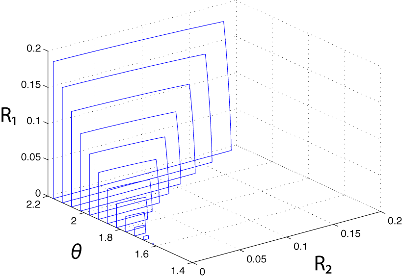
We would like to determine an interval for the parameter $\theta$ for which the channel exhibits “very strong” interference. In order to do so, we need to consider classical-quantum states of the following form:

\rho^{X_{1}X_{2}B_{1}B_{2}}\equiv\sum_{x_{1},x_{2}=0}^{1}p_{X_{1}}\left(x_{1}\right)p_{X_{2}}\left(x_{2}\right)\left|x_{1}\right\rangle\left\langle x_{1}\right|^{X_{1}}\otimes\\ \left|x_{2}\right\rangle\left\langle x_{2}\right|^{X_{2}}\otimes\psi_{x_{1},x_{2}}^{B_{1}B_{2}},

(49)

where $\psi_{x_{1},x_{2}}^{B_{1}B_{2}}$ is one of the pure output states in (45-48). We should then check whether the conditions in (42-43) hold for all distributions $p_{X_{1}}\left(x_{1}\right)$ and $p_{X_{2}}\left(x_{2}\right)$ . We can equivalently express these conditions in terms of von Neumann entropies as follows:

	$\displaystyle H\left(B_{1}\|X_{2}\right)_{\rho}-H\left(B_{1}\|X_{1}X_{2}\right)_{\rho}$	$\displaystyle\leq H\left(B_{2}\right)_{\rho}-H\left(B_{2}\|X_{1}\right)_{\rho},$
	$\displaystyle H\left(B_{2}\|X_{1}\right)_{\rho}-H\left(B_{2}\|X_{1}X_{2}\right)_{\rho}$	$\displaystyle\leq H\left(B_{1}\right)_{\rho}-H\left(B_{1}\|X_{2}\right)_{\rho},$

and thus, it suffices to calculate six entropies for states of the form in (49). After some straightforward calculations, we find the results in (50-54)

$\displaystyle H\left(B_{1}\|X_{1}X_{2}\right)_{\rho}$	$\displaystyle=H\left(B_{2}\|X_{1}X_{2}\right)_{\rho}=\left(p_{X_{1}}\left(0\right)p_{X_{2}}\left(1\right)+p_{X_{1}}\left(1\right)p_{X_{2}}\left(0\right)\right)H_{2}\left(\cos^{2}\left(\theta\right)\right),$	(50)
$\displaystyle H\left(B_{1}\right)_{\rho}$	$\displaystyle=H_{2}\left(p_{X_{1}}\left(0\right)+\left(p_{X_{1}}\left(1\right)p_{X_{2}}\left(0\right)-p_{X_{1}}\left(0\right)p_{X_{2}}\left(1\right)\right)\sin^{2}\left(\theta\right)\right),$	(51)
$\displaystyle H\left(B_{2}\right)_{\rho}$	$\displaystyle=H_{2}\left(p_{X_{2}}\left(0\right)+\left(p_{X_{1}}\left(0\right)p_{X_{2}}\left(1\right)-p_{X_{1}}\left(1\right)p_{X_{2}}\left(0\right)\right)\sin^{2}\left(\theta\right)\right),$	(52)
$\displaystyle H\left(B_{2}\|X_{1}\right)_{\rho}$	$\displaystyle=p_{X_{1}}\left(0\right)H_{2}\left(p_{X_{2}}\left(1\right)\cos^{2}\left(\theta\right)\right)+p_{X_{1}}\left(1\right)H_{2}\left(p_{X_{2}}\left(0\right)\cos^{2}\left(\theta\right)\right),$	(53)
$\displaystyle H\left(B_{1}\|X_{2}\right)_{\rho}$	$\displaystyle=p_{X_{2}}\left(0\right)H_{2}\left(p_{X_{1}}\left(1\right)\cos^{2}\left(\theta\right)\right)+p_{X_{2}}\left(1\right)H_{2}\left(p_{X_{1}}\left(0\right)\cos^{2}\left(\theta\right)\right),$	(54)

\mathbb{E}_{X_{1}^{n},X_{2}^{n},Q^{n}}\left\{\frac{1}{M_{1}M_{2}}\sum_{m_{1},m_{2}}\text{Tr}\left\{\left(I-\Lambda_{m_{1},m_{2}}\right)\rho_{X_{1}^{n}\left(m_{1}\right),X_{2}^{n}\left(m_{2}\right)}^{B_{1}^{n}}\right\}\right\}\leq\frac{\epsilon}{2},

(55)

\mathbb{E}_{X_{1}^{n},X_{2}^{n},Q^{n}}\left\{\frac{1}{M_{1}M_{2}}\sum_{m_{1},m_{2}}\text{Tr}\left\{\left(I-\Gamma_{m_{1},m_{2}}\right)\rho_{X_{1}^{n}\left(m_{1}\right),X_{2}^{n}\left(m_{2}\right)}^{B_{2}^{n}}\right\}\right\}\leq\frac{\epsilon}{2},

(56)

\mathbb{E}_{X_{1}^{n},X_{2}^{n},Q^{n}}\left\{\frac{1}{M_{1}M_{2}}\sum_{m_{1},m_{2}}\text{Tr}\left\{\left[\left(I-\Lambda_{m_{1},m_{2}}^{B_{1}^{n}}\right)+\left(I-\Gamma_{m_{1},m_{2}}^{B_{2}^{n}}\right)\right]\rho_{X_{1}^{n}\left(m_{1}\right),X_{2}^{n}\left(m_{2}\right)}^{B_{1}^{n}B_{2}^{n}}\right\}\right\}\leq\epsilon.

(57)

where $H_{2}\left(p\right)$ is the binary entropy function. We numerically checked for particular values of $\theta$ whether the conditions (42-43) hold for all distributions $p_{X_{1}}\left(x_{1}\right)$ and $p_{X_{2}}\left(x_{2}\right)$ , and we found that they hold when $\theta\in\left[0.96,2.18\right]\cup\left[4.10,5.32\right]$ (the latter interval in the union is approximately a shift of the first interval by $\pi$ ). The interval $\left[0.96,2.18\right]$ contains $\theta=\pi/2$ , the value of $\theta$ for which the capacity should vanish because the transformation is equivalent to a full SWAP (the channel at this point has “too strong” interference). We compute the capacity region given in Theorem 8 for several values of $\theta$ in the interval $\theta\in\left[\pi/2,2.18\right]$ (it is redundant to evaluate for other intervals because the capacity region is symmetric about $\pi/2$ and it is also equivalent for the two $\pi$ -shifted intervals $\left[0.96,2.18\right]$ and $\left[4.1,5.32\right]$ ). Figure 2 plots these capacity regions for several values of $\theta$ in the interval $\left[\pi/2,2.18\right]$ .

VI-A2 The Quantum Simultaneous Decoding Inner Bound

The two-sender quantum simultaneous decoder from Theorem 2 and Corollary 3 allows us to establish a non-trivial inner bound on the capacity of the quantum interference channel. The strategy is simply to consider the induced multiple access channels to each receiver and choose the rates low enough such that each receiver can decode the messages from both senders [2, 17]. This gives us the following theorem:

Theorem 10 (Simultaneous Decoding Inner Bound).

Let a ccqq quantum interference channel as in (41) be given. Then an achievable rate region is the union of all rates $R_{1}$ and $R_{2}$ satisfying the below inequalities:

	$\displaystyle R_{1}$	$\displaystyle\leq\min\left\{I\left(X_{1};B_{1}\|X_{2}Q\right)_{\rho},I\left(X_{1};B_{2}\|X_{2}Q\right)_{\rho}\right\},$
	$\displaystyle R_{2}$	$\displaystyle\leq\min\left\{I\left(X_{2};B_{2}\|X_{1}Q\right)_{\rho},I\left(X_{2};B_{1}\|X_{1}Q\right)_{\rho}\right\},$
	$\displaystyle R_{1}+R_{2}$	$\displaystyle\leq\min\left\{I\left(X_{1}X_{2};B_{1}\|Q\right)_{\rho},I\left(X_{1}X_{2};B_{2}\|Q\right)_{\rho}\right\},$

where the union is over input distributions $p_{Q}(q)\,p_{X_{1}|Q}\left(x_{1}|q\right)\,p_{X_{2}|Q}\left(x_{2}|q\right)$ .

Proof.

The proof exploits the two-sender quantum simultaneous decoder from Corollary 3. We first generate a time-sharing sequence $q^{n}$ according to the product distribution $p_{Q^{n}}(q^{n})$ . Let Sender 1 generate a codebook $\left\{X_{1}^{n}\left(m_{1}\right)\right\}_{m_{1}}$ independently and randomly according to the distribution $p_{X_{1}|Q}\left(x_{1}|q\right)$ , and let Sender 2 generate a codebook $\left\{X_{2}^{n}\left(m_{2}\right)\right\}_{m_{2}}$ with the distribution $p_{X_{2}|Q}\left(x_{2}|q\right)$ . The induced ccq multiple access channel to Receiver 1 is $x_{1},x_{2}\rightarrow\rho_{x_{1},x_{2}}^{B_{1}}$ , and the induced channel to Receiver 2 is $x_{1},x_{2}\rightarrow\rho_{x_{1},x_{2}}^{B_{2}}$ . Corollary 3 states that there exists a simultaneous decoding POVM $\left\{\Lambda_{m_{1},m_{2}}\right\}$ for Receiver 1 (corresponding to the random choice of code) such that (55) holds as long as

	$\displaystyle R_{1}$	$\displaystyle\leq I\left(X_{1};B_{1}\|X_{2}Q\right)_{\rho},$
	$\displaystyle R_{2}$	$\displaystyle\leq I\left(X_{2};B_{1}\|X_{1}Q\right)_{\rho},$
	$\displaystyle R_{1}+R_{2}$	$\displaystyle\leq I\left(X_{1}X_{2};B_{1}\|Q\right)_{\rho}.$

Similarly, we can invoke Corollary 3 to show that there is a simultaneous decoding POVM $\left\{\Gamma_{m_{1},m_{2}}\right\}$ for Receiver 2 such that (56) holds as long as

	$\displaystyle R_{1}$	$\displaystyle\leq I\left(X_{1};B_{2}\|X_{2}Q\right)_{\rho},$
	$\displaystyle R_{2}$	$\displaystyle\leq I\left(X_{2};B_{2}\|X_{1}Q\right)_{\rho},$
	$\displaystyle R_{1}+R_{2}$	$\displaystyle\leq I\left(X_{1}X_{2};B_{2}\|Q\right)_{\rho}.$

Thus, if we choose the rates as given in the statement of the theorem, then all six of the above inequalities are satisfied, implying that the inequality in (57) holds. Invoking the following operator inequality

I-\Lambda_{m_{1},m_{2}}^{B_{1}^{n}}\otimes\Gamma_{m_{1},m_{2}}^{B_{2}^{n}}\leq I-\Lambda_{m_{1},m_{2}}^{B_{1}^{n}}+I-\Gamma_{m_{1},m_{2}}^{B_{2}^{n}},

and derandomizing the expectation implies the existence of a code upon which all parties can agree. The agreed upon code has vanishing error probability in the asymptotic limit. ∎

VI-A3 Strong Interference

The simultaneous decoding inner bound from the previous section allows us to determine the capacity of a ccqq interference channel in the setting of “strong” interference (see page 6-12 of Ref. [17]). The conditions for “strong” interference are that the following information inequalities should hold for all distributions $p_{X_{1}}\left(x_{1}\right)$ and $p_{X_{2}}\left(x_{2}\right)$ :

	$\displaystyle I\left(X_{1};B_{1}\|X_{2}\right)_{\rho}$	$\displaystyle\leq I\left(X_{1};B_{2}\|X_{2}\right)_{\rho},$		(58)
	$\displaystyle I\left(X_{2};B_{2}\|X_{1}\right)_{\rho}$	$\displaystyle\leq I\left(X_{2};B_{1}\|X_{1}\right)_{\rho},$		(59)

where $\rho^{X_{1}X_{2}B_{1}B_{2}}$ is a state of the form in (44).

Theorem 11 (Strong Interference).

Let a ccqq quantum interference channel as in (41) be given which satisfies the condition of “strong interference” as in (58-59). Then the capacity region of such a channel is the union of all rates $R_{1}$ and $R_{2}$ satisfying the below inequalities:

	$\displaystyle R_{1}$	$\displaystyle\leq I\left(X_{1};B_{1}\|X_{2}Q\right)_{\rho},$
	$\displaystyle R_{2}$	$\displaystyle\leq I\left(X_{2};B_{2}\|X_{1}Q\right)_{\rho},$
	$\displaystyle R_{1}+R_{2}$	$\displaystyle\leq\min\left\{I\left(X_{1}X_{2};B_{1}\|Q\right)_{\rho},I\left(X_{1}X_{2};B_{2}\|Q\right)_{\rho}\right\},$

where the union is over input distributions $p_{Q}(q)\,p_{X_{1}|Q}\left(x_{1}|q\right)\,p_{X_{2}|Q}\left(x_{2}|q\right)$ .

Proof.

The proof exploits the quantum simultaneous decoding inner bound from Theorem 10 and the strong interference conditions in (58-59). The matching outer bound follows from similar reasoning as on page 6-13 of Ref. [17], though using quantum information inequalities rather than classical ones. ∎

VI-A4 Han-Kobayashi Achievable Rate Region

The following result provides an achievable rate region for the reliable transmission of classical data over a ccqq quantum interference channel (assuming Conjecture 4 regarding the existence of a quantum simultaneous decoder). We should mention that this result was subsequently proved by Sen [51] without relying on Conjecture 4. The statement of the theorem generates codes constructed from a single copy of a ccqq quantum interference channel. We can obtain the regularization of the region by blocking the channel $k$ times and constructing codes from the blocked channel (for any finite $k$ ).

Theorem 12 (Achievable Rate Region for the Quantum Interference Channel).

Assume Conjecture 4 holds. Let $\mathcal{S}_{\theta}$ be the set of tuples of non-negative reals $\left(S_{1},S_{2},T_{1},T_{2}\right)$ such that

$\displaystyle S_{1}$	$\displaystyle\leq I\left(U_{1};B_{1}\|W_{1}W_{2}\right)_{\theta},$	(60)
$\displaystyle T_{1}$	$\displaystyle\leq I\left(W_{1};B_{1}\|U_{1}W_{2}\right)_{\theta},$	(61)
$\displaystyle T_{2}$	$\displaystyle\leq I\left(W_{2};B_{1}\|U_{1}W_{1}\right)_{\theta},$	(62)
$\displaystyle S_{1}+T_{1}$	$\displaystyle\leq I\left(U_{1}W_{1};B_{1}\|W_{2}\right)_{\theta},$	(63)
$\displaystyle S_{1}+T_{2}$	$\displaystyle\leq I\left(U_{1}W_{2};B_{1}\|W_{1}\right)_{\theta},$	(64)
$\displaystyle T_{1}+T_{2}$	$\displaystyle\leq I\left(W_{1}W_{2};B_{1}\|U_{1}\right)_{\theta},$	(65)
$\displaystyle S_{1}+T_{1}+T_{2}$	$\displaystyle\leq I\left(U_{1}W_{1}W_{2};B_{1}\right)_{\theta},$	(66)

$\displaystyle S_{2}$	$\displaystyle\leq I\left(U_{2};B_{2}\|W_{1}W_{2}\right)_{\theta},$	(67)
$\displaystyle T_{1}$	$\displaystyle\leq I\left(W_{1};B_{2}\|U_{2}W_{2}\right)_{\theta},$	(68)
$\displaystyle T_{2}$	$\displaystyle\leq I\left(W_{2};B_{2}\|U_{2}W_{1}\right)_{\theta},$	(69)
$\displaystyle S_{2}+T_{1}$	$\displaystyle\leq I\left(U_{2}W_{1};B_{2}\|W_{2}\right)_{\theta},$	(70)
$\displaystyle S_{2}+T_{2}$	$\displaystyle\leq I\left(U_{2}W_{2};B_{2}\|W_{1}\right)_{\theta},$	(71)
$\displaystyle T_{1}+T_{2}$	$\displaystyle\leq I\left(W_{1}W_{2};B_{2}\|U_{2}\right)_{\theta},$	(72)
$\displaystyle S_{2}+T_{1}+T_{2}$	$\displaystyle\leq I\left(U_{2}W_{1}W_{2};B_{2}\right)_{\theta},$	(73)

where $\theta$ is a state of the following form:

\theta^{U_{1}U_{2}W_{1}W_{2}B_{1}B_{2}}\equiv\\ \sum_{u_{1},u_{2},w_{1},w_{2}}p_{U_{1}}\left(u_{1}\right)p_{U_{2}}\left(u_{2}\right)p_{W_{1}}\left(w_{1}\right)p_{W_{2}}\left(w_{2}\right)\\ \left|u_{1}\right\rangle\left\langle u_{1}\right|^{U_{1}}\otimes\left|u_{2}\right\rangle\left\langle u_{2}\right|^{U_{2}}\otimes\left|w_{1}\right\rangle\left\langle w_{1}\right|^{W_{1}}\otimes\left|w_{2}\right\rangle\left\langle w_{2}\right|^{W_{2}}\otimes\\ \rho_{f_{1}\left(u_{1},w_{1}\right),f_{2}\left(u_{2},w_{2}\right)}^{B_{1}B_{2}},

(74)

and $f_{1}:\mathcal{U}_{1}\times\mathcal{W}_{1}\rightarrow\mathcal{X}_{1}$ and $f_{2}:\mathcal{U}_{2}\times\mathcal{W}_{2}\rightarrow\mathcal{X}_{2}\mathcal{\ }$ are arbitrary functions. A rate region is achievable if for all $\epsilon>0$ and sufficiently large $n$ , there exists a code with vanishing average error probability as given in (75) where $\rho_{f_{1}^{n}\left(u_{1}^{n}\left(i\right),w_{1}^{n}\left(k\right)\right),f_{2}^{n}\left(u_{2}^{n}\left(j\right),w_{2}^{n}\left(m\right)\right)}$ represents the encoded state, $i$ is a “personal” message of Sender 1, $k$ is a “common” message of Sender 1, $j$ is a “personal” message of Sender 2, $m$ is a “common” message of Sender 2, $\left\{\Lambda_{i,k,m}\right\}$ is the POVM of Receiver 1, and $\left\{\Gamma_{j,k,m}\right\}$ is the POVM of Receiver 2. An achievable rate region for the quantum interference channel $x_{1},x_{2}\rightarrow\rho_{x_{1},x_{2}}$ is the set of all rates $\left(S_{1}+T_{1},S_{2}+T_{2}\right)$ where $\left(S_{1},S_{2},T_{1},T_{2}\right)\in\mathcal{S}_{\theta}$ and $\theta$ is a state of the form in (74).

\frac{1}{L_{1}L_{2}M_{1}M_{2}}\sum_{i,j,k,m}\text{Tr}\left\{\left(I-\Lambda_{i,k,m}\otimes\Gamma_{j,k,m}\right)\rho_{f_{1}^{n}\left(u_{1}^{n}\left(i\right),w_{1}^{n}\left(k\right)\right),f_{2}^{n}\left(u_{2}^{n}\left(j\right),w_{2}^{n}\left(m\right)\right)}\right\}\leq\epsilon,

(75)

	$\displaystyle\mathbb{E}\left\{\frac{1}{L_{1}M_{1}M_{2}}\sum_{i,k,m}\text{Tr}\left\{\left(I-\Lambda_{i,k,m}\right)\rho_{f_{1}^{n}\left(u_{1}^{n}\left(i\right),w_{1}^{n}\left(k\right)\right),f_{2}^{n}\left(u_{2}^{n}\left(j\right),w_{2}^{n}\left(m\right)\right)}\right\}\right\}$	$\displaystyle\leq\frac{\epsilon}{2},$		(76)
	$\displaystyle\mathbb{E}\left\{\frac{1}{L_{2}M_{1}M_{2}}\sum_{j,k,m}\text{Tr}\left\{\left(I-\Gamma_{j,k,m}\right)\rho_{f_{1}^{n}\left(u_{1}^{n}\left(i\right),w_{1}^{n}\left(k\right)\right),f_{2}^{n}\left(u_{2}^{n}\left(j\right),w_{2}^{n}\left(m\right)\right)}\right\}\right\}$	$\displaystyle\leq\frac{\epsilon}{2}.$		(77)

\frac{1}{L_{1}L_{2}M_{1}M_{2}}\sum_{i,j,k,m}\text{Tr}\left\{\left[\left(I-\Lambda_{i,k,m}\right)+\left(I-\Gamma_{j,k,m}\right)\right]\rho_{f_{1}^{n}\left(u_{1}^{n}\left(i\right),w_{1}^{n}\left(k\right)\right),f_{2}^{n}\left(u_{2}^{n}\left(j\right),w_{2}^{n}\left(m\right)\right)}\right\}\leq\epsilon.

(78)

Proof.

We merely need to set up how the senders select a code randomly and the rest of the proof follows by reasoning similar to that of Han and Kobayashi [20], although we require an application of Conjecture 4. Figure 3 depicts the Han-Kobayashi coding strategy. Sender 1 generates $2^{nS_{1}}$ “personal” codewords $\left\{u_{1}^{n}\left(i\right)\right\}_{i\in\left[1,\ldots,L_{1}\right]}$ according to the distribution $p_{U_{1}^{n}}\left(u_{1}^{n}\right)$ and $2^{nT_{1}}$ “common” codewords $\left\{w_{1}^{n}\left(k\right)\right\}_{k\in\left[1,\ldots,M_{1}\right]}$ according to the distribution $p_{W_{1}^{n}}\left(w_{1}^{n}\right)$ . Sender 2 generates $2^{nS_{2}}$ “personal” codewords $\left\{u_{2}^{n}\left(j\right)\right\}_{j\in\left[1,\ldots,L_{2}\right]}$ according to the distribution $p_{U_{2}^{n}}\left(u_{2}^{n}\right)$ and $2^{nT_{2}}$ “common” codewords $\left\{w_{2}^{n}\left(m\right)\right\}_{m\in\left[1,\ldots,M_{2}\right]}$ according to the distribution $p_{W_{2}^{n}}\left(w_{2}^{n}\right)$ . Receiver 1 “sees” a three-input multiple access channel after tracing over Receiver 2’s system, and the relevant state for randomly selecting a code is many copies of Tr ${}_{B_{2}}\left\{\theta^{U_{1}U_{2}W_{1}W_{2}B_{1}B_{2}}\right\}$ . Receiver 2 “sees” a three-input multiple access channel after tracing over Receiver 1’s system, and the relevant state for randomly selecting a code is many copies of Tr ${}_{B_{1}}\left\{\theta^{U_{1}U_{2}W_{1}W_{2}B_{1}B_{2}}\right\}$ . Observe that these states are of the form needed to apply Conjecture 4. A direct application of Conjecture 4 to the state Tr ${}_{B_{2}}\left\{\theta^{U_{1}U_{2}W_{1}W_{2}B_{1}B_{2}}\right\}$ shows that there exists a POVM that can distinguish the common messages of both senders and the personal message of Sender 1 provided that (60-66) hold. Similarly, a direct application of Conjecture 4 to the state Tr ${}_{B_{1}}\left\{\theta^{U_{1}U_{2}W_{1}W_{2}B_{1}B_{2}}\right\}$ shows that there exists a POVM that can distinguish the common messages of both senders and the personal message of Sender 2 provided that (67-73) hold. We obtain the bounds in (76-77) on the expectation of the average error probability for each code, provided that the rates satisfy the inequalities in (60-73). We then sum the two expectations of the average error probabilities together. Since the expectation is bounded above by some arbitrarily small, positive number $\epsilon$ , there exists a particular code such that the bound in (78) holds. We finally apply the bound

I-\Lambda_{i,k,m}\otimes\Gamma_{j,k,m}\leq\left(I-\Lambda_{i,k,m}\right)+\left(I-\Gamma_{j,k,m}\right),

that holds for any two commuting positive operators each less than or equal to the identity, to get the bound in (75) on the average error probability. This demonstrates that any rate pair $\left(S_{1}+T_{1},S_{2}+T_{2}\right)$ is achievable for the quantum interference channel (up to Conjecture 4). ∎

Extending the strategies of the previous section and this section to the case of a quantum interference channel with quantum inputs and quantum outputs is straightforward. The senders have the choice to prepare density operators, conditional on classical inputs, as input to this general quantum interference channel, and this extra preprocessing for preparation effectively induces a ccqq quantum interference channel for which they are coding. Thus, the achievable rate regions include an extra degree of freedom in the choice of density operators at the inputs. Also, Theorems 8 and 11 are no longer optimal in the case of “very strong” or “strong” interference because entanglement at the individual encoders could increase capacity for certain interference channels [25].

VI-A5 Rates achievable by successive decoding

In Section V-A on the multiple access channel, we saw that a successive decoding strategy can be used to achieve certain rate tuples. Then, by time-sharing between the different codes achieving these rates, it is possible to construct good codes for the full capacity region of the multiple access channel. To obtain an inner bound for the interference channel, one could try to use these codes for the two induced multiple access channels. However, this strategy is not well-adapted in this setting because the codebooks obtained for the two multiple access channels are not necessarily the same for fixed rates $R_{1}$ and $R_{2}$ . In addition, decoding a codebook constructed by time-sharing between two codebooks ${\cal C}_{1}$ and ${\cal C}_{2}$ assumes that both ${\cal C}_{1}$ and ${\cal C}_{2}$ are decodable, and these codes do in general depend on the properties of the channel for which one is coding. For this reason, a time-sharing strategy that works for one of the induced multiple access channels might not work for the other one.

It is however possible to use successive decoding strategies for an interference channel in the following way. We start by considering a strategy where both receivers are asked to decode both messages, i.e., we are dealing with the compound multiple access channel. Such a strategy defines an achievable rate region known as the “successive decoding inner bound” for the interference channel (c.f., page 6-7 of Ref. [17]). Suppose that Receiver 1 starts by decoding the message of Sender 2 and then the message of Sender 1, and Receiver 2 does the same. We can describe the decode orderings of the receivers by the two permutations $\pi_{1}=(2,1)$ and $\pi_{2}=(2,1)$ . In this case, we know that the random code defined by picking $2^{nR_{1}}$ and $2^{nR_{2}}$ codewords independently according to the product distributions $p^{n}_{X^{n}_{1}}$ and $p^{n}_{X^{n}_{2}}$ is decodable on average for Receiver 1 provided $R_{1}<I(X_{1};B_{1}|X_{2})$ and $R_{2}<I(X_{2};B_{1})$ . Moreover, it is decodable on average for Receiver 2 provided $R_{1}<I(X_{2};B_{2}|X_{1})$ and $R_{2}<I(X_{2};B_{2})$ . Thus, the rate pairs $R_{1}<\min\{I(X_{1};B_{1}|X_{2}),I(X_{1};B_{2}|X_{2}\})$ and $R_{2}<\min\{I(X_{2};B_{1}),I(X_{2};B_{2})\}$ are all achievable for the interference channel. Recall that Receiver 2 is actually not interested in the message sent by Sender 1. The only reason to decode the message of Sender 1 is to be able to decode the message of Sender 2 at a higher rate. It is thus useless to require Receiver 2 to decode the message of Sender 1 after decoding the message of Sender 2.

The above ordering shows that the rate pairs $R_{1},R_{2}$ where $R_{1}<I(X_{1};B_{1}|X_{2})$ and $R_{2}<\min\{I(X_{2};B_{1}),$ $I(X_{2};B_{2})\}$ are all achievable for the interference channel. Naturally, we can do the same for all decode orderings $\pi_{1}$ , $\pi_{2}$ and we can achieve rates arbitrarily close to the following points:

$\displaystyle P_{1}$	$\displaystyle=(I(X_{1};B_{1}\|X_{2}),\min\{I(X_{2};B_{1}),I(X_{2};B_{2})\}),$	(79)
$\displaystyle P_{2}$	$\displaystyle=(\min\{I(X_{1};B_{1}\|X_{2}),I(X_{1};B_{2})\},$
	$\displaystyle\,\,\,\,\,\,\,\,\,\,\,\min\{I(X_{2};B_{1}),I(X_{2};B_{2}\|X_{1})\}),$	(80)
$\displaystyle P_{3}$	$\displaystyle=(\min\{I(X_{1};B_{1}),I(X_{1};B_{2})\},I(X_{2};B_{2}\|X_{1})),$	(81)
$\displaystyle P_{4}$	$\displaystyle=(I(X_{1};B_{1}),I(X_{2};B_{2})).$	(82)

Of course, one can use time-sharing between these different codes for the interference channel to obtain other achievable rates. These rates are illustrated in the RHS of Figure 4.

Fig. 4: These plots show achievable rates regions for the interference channel for simultaneous decoding and successive decoding strategies with fixed input distributions. Using a simultaneous decoding strategy, it is possible to achieve the intersection of the two regions of the corresponding multiple access channels. Using a successive decoding strategy, we obtain four achievable rate points that correspond to the possible decoding orders for the two multiple access channels. The solid red and blue lines outline the different multiple access channel achievable rate regions, and the shaded gray areas outline the achievable rate regions for the two different decoding strategies.

Improving rates using rate-splitting. As can be seen in Figure 4, the region defined by the convex hull of the points (79)-(82) is, in general, smaller than the simultaneous decoding inner bound. A natural question is whether it is possible to obtain the simultaneous decoding inner bound, or even more generally, the full Han-Kobayashi rate region using a more sophisticated successive decoding argument. There exists an attempt to answer this question for the classical interference channel [52]. This attempt exploits rate-splitting [19] and a careful analysis of the geometrical structure of the four-dimensional region (corresponding to the two natural multiple access channels defined by the interference channel) that projects down to the two-dimensional Chong-Motani-Garg region [9]. The Chong-Motani-Garg region is known to be equivalent to the Han-Kobayashi region when considering all possible input distributions [10, 35]. The argument of Ref. [52] rests on an assumption that the change of the code distribution dictated by applying the rate-splitting technique at the convenience of some receiver does not affect the other receiver’s decoding ability. Unfortunately, this assumption does not hold in general. We explain this issue in greater detail in the following paragraphs.

Consider an input distribution $p_{X}\left(x\right)$ on some alphabet $\mathcal{X}$ . Let $\mathcal{C}_{0}$ be the codebook obtained by picking $2^{nR}$ independent codewords of length $n$ distributed according to $p_{X^{n}}\left(x^{n}\right)$ . A split of $p_{X}\left(x\right)$ consists of a function $f:\mathcal{X}\times\mathcal{X}\rightarrow\mathcal{X}$ and distributions $p_{U}\left(u\right)$ and $p_{V}\left(v\right)$ such that $f(U,V)\sim p_{X}\left(x\right)$ where $U\sim p_{U}\left(u\right)$ and $V\sim p_{V}\left(v\right)$ are independent [19]. The rate-splitting technique in general refers to following coding strategy. Generate a code $\mathcal{C}_{U}$ from the distribution $p_{U^{n}}\left(u^{n}\right)$ consisting of $2^{nR_{U}}$ independent codewords and a code $\mathcal{C}_{V}$ from the distribution $p_{V^{n}}\left(v^{n}\right)$ consisting of $2^{nR_{V}}$ independent codewords, where $R_{U}+R_{V}=R$ . The codebook $\mathcal{C}_{\text{split}}$ is defined as $\{f^{n}(u^{n},v^{n}):(u^{n},v^{n})\in\mathcal{C}_{U}\times\mathcal{C}_{V}\}$ . Note that $\mathcal{C}_{\text{split}}$ contains $2^{n(R_{U}+R_{V})}=2^{nR}$ codewords. Furthermore, the codewords of $\mathcal{C}_{\text{split}}$ are all distributed according to $p_{X^{n}}\left(x^{n}\right)$ . The difference between this codebook and $\mathcal{C}_{0}$ is that the codewords in $\mathcal{C}_{\text{split}}$ are not pairwise independent because two codewords in $\mathcal{C}_{\text{split}}$ could arise from the same $u^{n}$ and $v_{1}^{n}\neq v_{2}^{n}$ where $u^{n}\in\mathcal{C}_{U}$ and $v_{1}^{n},v_{2}^{n}\in\mathcal{C}_{V}$ .

Now we describe how to choose the rates $R_{U}$ and $R_{V}$ . Suppose that $R=I(X;Y)$ where $Y$ is the output of a channel on input $X$ . Then a natural choice for $R_{U}$ and $R_{V}$ is $R_{U}=I(U;Y)$ and $R_{V}=I(V;Y|U)$ because $I(X;Y)=I(U;Y)+I(V;Y|U)$ . Observe that the values of $R_{U}$ and $R_{V}$ depend on the channel. Consider now a code for an interference channel where $X$ is to be decoded by both receivers. Such an additional requirement arises for example for the common messages in the Han-Kobayashi inner bound strategy. Let $R=I(X;Y_{1})$ and $R\leq I(X;Y_{2})$ . Using the codebook $\mathcal{C}_{0}$ , both receivers are able to decode $X$ . However, when coding for a multiple access channel with output $Y_{1}$ , we might want to split $p_{X}\left(x\right)$ into $p_{U}\left(u\right)$ and $p_{V}\left(v\right)$ and use the codebook $\mathcal{C}_{\text{split}}$ for $X$ with rates $R_{U}=I(U;Y_{1})$ and $R_{V}=I(V;Y_{1}|U)$ instead of using $\mathcal{C}_{0}$ [19]. We perform this split because we want to get a non-corner point of the rate region for the multiple access channel with output $Y_{1}$ only using successive decoding. In this case, Receiver $~1$ can decode with small error probability. We should however keep in mind that we are coding for an interference channel and we also want Receiver $~2$ to decode $X$ . The problem is that it is possible that $R_{U}=I(U;Y_{1})>I(U;Y_{2})$ , in which case Receiver $~2$ cannot decode $U$ and thus cannot decode $X$ . In this case, the code obtained by splitting according to the first receiver’s prescription is not a good code for the second receiver and hence not a good code for the interference channel.

One can however use rate-splitting to obtain potentially better rates than the four points (79)-(82) that can be achieved using a simple successive decoding strategy. In fact, splitting the two inputs of the interference channel as in the Han-Kobayashi strategy into a “personal” and a “common” part and requiring each receiver to decode both common parts induces two 3-user multiple access channels. One can naturally use all $6\times 6$ pairs of decoding orders to obtain an achievable rate pair for the interference channel. Figure 5 shows some rates that can be achieved using such a strategy for a classical Gaussian interference channel.

Fig. 5: These two figures plot rate pairs that the senders and receivers in a classical Gaussian interference channel can achieve with successive decoding and rate-splitting (SD+RS). The figures compare these rates with those achievable by the Han-Kobayashi (HK) coding strategy, while also plotting the regions corresponding to the two induced multiple access channels to each receiver (MAC1 and MAC2). The LHS figure demonstrates that, for a particular choice of signal to noise (SNR) and interference to noise (INR) parameters (SNR1 = 1.7, SNR2 = 2, INR1 = 3.4, INR2 = 4), successive decoding with rate-splitting does not perform as well as the Han-Kobayashi strategy. The RHS figure demonstrates that, for a different choice of parameters (SNR1 = 343, SNR2 = 296, INR1 = 5, INR2 = 5), the two strategies perform equally well.

Of course, it is possible to split the inputs even further, leading to two six-user multiple access channels. An interesting open question is to determine whether such a strategy can achieve the full Han-Kobayashi region—such a result would be important for the quantum interference channel because it would immediately lead to a way to achieve the analogous Han-Kobayashi region without employing Conjecture 4.

VI-B Outer Bound

We also give a simple outer bound for the capacity of the quantum interference channel. This result follows naturally from a classical result of Sato’s [46], where he observes that any code for the quantum interference channel also gives codes for three quantum multiple access channel subproblems, one for Receiver 1, another for Receiver 2, and a third for the two receivers considered together. Thus, if we have an outer bound on the underlying quantum multiple access channel capacities [62], then we can trivially get an outer bound on the quantum interference channel capacity. We omit the following theorem’s proof because of its similarity to Sato’s proof.

Theorem 13.

Consider the Sato region defined as follows:

\mathcal{R}_{\text{Sato}}(\mathcal{N})\triangleq\bigcup_{p_{Q}(q)p_{1}(x_{1}|q)p_{2}(x_{2}|q)}\{(R_{1},R_{2})\},

(83)

where $R_{1}$ and $R_{2}$ are rates satisfying the following inequalities:

$\displaystyle R_{1}$	$\displaystyle\leq I(X_{1};B_{1}\|X_{2}Q)_{\theta},$	(84)
$\displaystyle R_{2}$	$\displaystyle\leq I(X_{2};B_{2}\|X_{1}Q)_{\theta},$	(85)
$\displaystyle R_{1}+R_{2}$	$\displaystyle\leq I(X_{1}X_{2};B_{1}B_{2}\|Q)_{\theta}.$	(86)

The above entropic quantities are with respect to the following state

\theta^{QX_{1}X_{2}B_{1}B_{2}}\equiv\sum_{q,x_{1},x_{2}}p_{Q}(q)p_{1}(x_{1}|q)p_{2}(x_{2}|q)\ |q\rangle\langle q|^{Q}\otimes\\ |x_{1}\rangle\langle x_{1}|^{X_{1}}\otimes|x_{2}\rangle\langle x_{2}|^{X_{2}}\otimes\rho_{x_{1}x_{2}}^{B_{1}B_{2}}.

(87)

Then the region $\mathcal{R}_{\text{Sato}}$ forms an outer bound on the capacity region of the quantum interference channel.

VII The Connection to Unitary Gate Capacities

Considerable effort has been devoted to the problem of establishing the information theoretic capacities of an interaction $U:C\otimes D\rightarrow C\otimes D$ between two quantum systems [3, 22, 23, 24]. One imagines that Charlie controls the system represented by the $C$ Hilbert space while Donna controls $D$ , and that they would like to exploit $U$ to communicate or establish correlations. (More generally, the interaction might be modeled by a Hamiltonian, but that situation can be reduced to the unitary case.) Since $U$ has two inputs and two outputs, this is a special case of a quantum interference channel, and so Theorem 12 will yield achievable rates for classical communication over $U$ and, as we shall see, significantly more.

When $U$ is thought of as an interference channel (say, with quantum inputs $A_{1}$ and $A_{2}$ and quantum outputs $B_{1}$ and $B_{2}$ as discussed at the end of Section VI-A4), Charlie plays the roles of both Sender 1 and Receiver 2, while Donna plays the roles of both Sender 2 and Receiver 1 (Figure 6 depicts this communication scenario). Theorem 12 then gives achievable rates for simultaneous Charlie-to-Donna and Donna-to-Charlie classical communication over $U$ . Indeed, it appears to provide the first nontrivial protocol accomplishing this task for general bidirectional channels. (Earlier protocols assumed free shared entanglement between Charlie and Donna [3].) To apply the theorem, it suffices to identify $A_{1}=B_{2}=C$ and $A_{2}=B_{1}=D$ in the interference channel $\mathcal{N}^{A_{1}A_{2}\rightarrow B_{1}B_{2}}(\rho)=U\rho U^{\dagger}$ . The communication rates achievable for the $\theta$ -SWAP channel of Example 9, for instance, apply equally well to this setting.

The fact that Charlie and Donna are each both sender and receiver gives them some flexibility not available for general interference channels. Most importantly, in this “bidirectional” setting, they are permitted to use $U$ sequentially, reinserting their outputs into the channel in each successive round [3]. Codes for standard interference channels, on the other hand, cannot take advantage of this flexibility, and so finding the optimal trade-off between forward and backward communication will likely require codes specifically tailored to the bidirectional setting.

As an interference channel, $U$ is also special because the only noise is due to interference: the channel itself is noiseless. Because $U$ does not leak information to an environment, communication can be made coherent at essentially no cost. This allowed Harrow and Leung to establish the following remarkable result, which we state informally using resource inequalities [13]. Recall that $[c\rightarrow c]$ represents a classical bit of communication from Charlie to Donna, $[q\rightarrow q]$ one qubit of communication from Charlie to Donna, and $[q\rightarrow qq]$ one cobit from Charlie to Donna, that is, the isometry $\sum_{x}\alpha_{x}|x\rangle^{C}\rightarrow\sum_{x}\alpha_{x}|x\rangle^{C}|x\rangle^{D}$ . $[c\leftarrow c]$ [21], $[q\leftarrow q]$ and $[qq\leftarrow q]$ represent the same resources but with Donna the sender and Charlie the receiver. Finally, $[qq]$ represents a single shared ebit. For a rigorous definition of resource inequalities, see [13] and [24].

Theorem 14 (Harrow and Leung [22]).

For any bipartite unitary (or isometry) $U$ and $R_{1},R_{2}\geq 0$ , each of the following resource inequalities is equivalent:

$\displaystyle\langle U\rangle$	$\displaystyle\geq R_{1}[c\rightarrow c]+R_{2}[c\leftarrow c]+E[qq],$	(88)
$\displaystyle\langle U\rangle$	$\displaystyle\geq R_{1}[q\rightarrow qq]+R_{2}[qq\leftarrow q]+E[qq],$	(89)
$\displaystyle\langle U\rangle$	$\displaystyle\geq\frac{R_{1}}{2}[q\rightarrow q]+\frac{R_{2}}{2}[q\leftarrow q]+\left(E-\frac{R_{1}+R_{2}}{2}\right)[qq].$	(90)

Note that the inequalities need only hold in the limit of a large number of uses of $U$ and might require the catalytic use of resources. Still, they imply that for bidirectional channels, the codes we have designed for sending classical data can also be used to send cobits, ebits and even qubits. In particular, any rates of classical communication that are achievable can automatically be upgraded to cobit communication rates. While our codes should be effective for cobit communication, they have not been designed to generate entanglement. While they can do so at the rate $R_{1}+R_{2}$ by virtue of the fact that a cobit can be used to generate an ebit, that process might be inefficient. In fact, Harrow and Leung have even exhibited a particular channel with $C$ and $D$ each consisting of $k$ qubits for which $R_{1}+R_{2}$ can never exceed $O(\log k)$ but for which $E$ can be larger than $k-1$ [23]. For that channel, our codes would produce an amount of entanglement exponentially smaller than optimal. Rectifying that problem would require modifying the interference channel codes we developed in this article to also establish shared randomness between the two receivers; such shared randomness would automatically become entanglement in the bidirectional unitary setting.

VIII Outlook

Calculating the capacity of the interference channel in the classical setting has been an open problem for many years now, and calculating the capacity of the quantum interference channel will be at least as difficult to solve. We have proved that a quantum simultaneous decoder exists for a multiple access channel with two senders, and we have given some evidence that it should exist for channels with three senders. This conjecture holds at least in the case of a quantum multiple access channel in which certain averages of the channel outputs commute. If this conjecture holds in the general case, it immediately implies that the Han-Kobayashi rate region, expressed in terms of Holevo information quantities, is an achievable rate region for the quantum interference channel. Note that even though the general conjecture is still open, the Han-Kobayashi rate region was recently shown to be achievable [51].

Even though Theorem 12 is now known to hold [51], it would still be very interesting to prove Conjecture 4. A proof of this conjecture would probably have important consequences for multiuser quantum information theory since it would allow for many classical information theory results based on simultaneous decoding to be adapted to the quantum setting. It could also likely prove an entanglement-assisted version of a quantum simultaneous decoder by exploiting the coding techniques from Ref. [33], and this would in turn lead to another interesting generalization of the Han-Kobayashi rate region where we assume that senders share entanglement with their partner receivers. Ref. [63] made progress in this direction by proving the existence of a quantum simultaneous decoder for an entanglement-assisted quantum multiple access channel with two senders, though the three-sender case is still open.

Also, just as there are many different capacities for a single-sender single-receiver quantum channel, we would expect that there are many interesting capacities that we could study for a quantum interference channel. In fact, we initially attempted to use some of the well-known decoupling techniques for the case of quantum information transmission over the quantum interference channel [28, 1], but we were not able to achieve non-trivial rates.

Another important question to consider for the quantum interference channel is as follows: Is there anything that quantum mechanics can offer to improve upon the Han-Kobayashi achievable rate region? Quantum effects might play some unexpected role for the quantum interference channel and allow us to achieve a rate region that is superior to the well-known Han-Kobayashi rate region.

Finally, it could be that quantum simultaneous decoding is not necessary in order to achieve the Han-Kobayashi region. In fact, our first attempt at the proof of Theorem 12 was to quantize the successive decoding method from Ref. [52], by exploiting the coding techniques from Refs. [62, 14] tailored for classical communication. But we found an issue with the technique in Ref. [52] even for the classical interference channel because rate-splitting at the convenience of one receiver affects the other receiver’s decoding abilities. Thus, it remains open to determine if a successive decoding strategy can achieve the Han-Kobayashi rate region.

We acknowledge discussions with Charlie Bennett, Kamil Brádler, Nilanjana Datta, Frédéric Dupuis, Saikat Guha, Aram Harrow, Min-Hsiu Hsieh, Debbie Leung, Will Matthews, Marco Piani, Eren Şaşoğlu, Graeme Smith, John Smolin, Jon Tyson, Mai Vu, Andreas Winter, and Shen Chen Xu. P. Hayden acknowledges support from the Canada Research Chairs program, the Perimeter Institute, CIFAR, FQRNT’s INTRIQ, MITACS, NSERC, ONR through grant N000140811249, and QuantumWorks. M. M. Wilde acknowledges support from the MDEIE (Québec) PSR-SIIRI international collaboration grant. I. Savov acknowledges support from FQRNT and NSERC.

Appendix A Typical Sequences and Typical Subspaces

Consider a density operator $\rho$ with the following spectral decomposition:

\rho=\sum_{x}p_{X}\left(x\right)\left|x\right\rangle\left\langle x\right|.

The weakly typical subspace is defined as the span of all vectors such that the sample entropy $\overline{H}\left(x^{n}\right)$ of their classical label is close to the true entropy $H\left(X\right)$ of the distribution $p_{X}\left(x\right)$ [41, 60]:

T_{\delta}^{X^{n}}\equiv\text{span}\left\{\left|x^{n}\right\rangle:\left|\overline{H}\left(x^{n}\right)-H\left(X\right)\right|\leq\delta\right\},

where

	$\displaystyle\overline{H}\left(x^{n}\right)$	$\displaystyle\equiv-\frac{1}{n}\log\left(p_{X^{n}}\left(x^{n}\right)\right),$
	$\displaystyle H\left(X\right)$	$\displaystyle\equiv-\sum_{x}p_{X}\left(x\right)\log p_{X}\left(x\right).$

The projector $\Pi_{\rho,\delta}^{n}$ onto the typical subspace of $\rho$ is defined as

\Pi_{\rho,\delta}^{n}\equiv\sum_{x^{n}\in T_{\delta}^{X^{n}}}\left|x^{n}\right\rangle\left\langle x^{n}\right|,

where we have “overloaded” the symbol $T_{\delta}^{X^{n}}$ to refer also to the set of $\delta$ -typical sequences:

T_{\delta}^{X^{n}}\equiv\left\{x^{n}:\left|\overline{H}\left(x^{n}\right)-H\left(X\right)\right|\leq\delta\right\}.

The three important properties of the typical projector are as follows:

	$\displaystyle\text{Tr}\left\{\Pi_{\rho,\delta}^{n}\rho^{\otimes n}\right\}$	$\displaystyle\geq 1-\epsilon,$
	$\displaystyle\text{Tr}\left\{\Pi_{\rho,\delta}^{n}\right\}$	$\displaystyle\leq 2^{n\left[H\left(X\right)+\delta\right]},$
	$\displaystyle 2^{-n\left[H\left(X\right)+\delta\right]}\Pi_{\rho,\delta}^{n}$	$\displaystyle\leq\Pi_{\rho,\delta}^{n}\rho^{\otimes n}\Pi_{\rho,\delta}^{n}\leq 2^{-n\left[H\left(X\right)-\delta\right]}\Pi_{\rho,\delta}^{n},$

where the first property holds for arbitrary $\epsilon,\delta>0$ and sufficiently large $n$ .

Consider an ensemble $\left\{p_{X}\left(x\right),\rho_{x}\right\}_{x\in\mathcal{X}}$ of states. Suppose that each state $\rho_{x}$ has the following spectral decomposition:

\rho_{x}=\sum_{y}p_{Y|X}\left(y|x\right)\left|y_{x}\right\rangle\left\langle y_{x}\right|.

Consider a density operator $\rho_{x^{n}}$ which is conditional on a classical sequence $x^{n}\equiv x_{1}\cdots x_{n}$ :

\rho_{x^{n}}\equiv\rho_{x_{1}}\otimes\cdots\otimes\rho_{x_{n}}.

We define the weak conditionally typical subspace as the span of vectors (conditional on the sequence $x^{n}$ ) such that the sample conditional entropy $\overline{H}\left(y^{n}|x^{n}\right)$ of their classical labels is close to the true conditional entropy $H\left(Y|X\right)$ of the distribution $p_{Y|X}\left(y|x\right)p_{X}\left(x\right)$ [41, 60]:

T_{\delta}^{Y^{n}|x^{n}}\equiv\text{span}\left\{\left|y_{x^{n}}^{n}\right\rangle:\left|\overline{H}\left(y^{n}|x^{n}\right)-H\left(Y|X\right)\right|\leq\delta\right\},

where

	$\displaystyle\overline{H}\left(y^{n}\|x^{n}\right)$	$\displaystyle\equiv-\frac{1}{n}\log\left(p_{Y^{n}\|X^{n}}\left(y^{n}\|x^{n}\right)\right),$
	$\displaystyle H\left(Y\|X\right)$	$\displaystyle\equiv-\sum_{x}p_{X}\left(x\right)\sum_{y}p_{Y\|X}\left(y\|x\right)\log p_{Y\|X}\left(y\|x\right).$

The projector $\Pi_{\rho_{x^{n}},\delta}$ onto the weak conditionally typical subspace of $\rho_{x^{n}}$ is as follows:

\Pi_{\rho_{x^{n}},\delta}\equiv\sum_{y^{n}\in T_{\delta}^{Y^{n}|x^{n}}}\left|y_{x^{n}}^{n}\right\rangle\left\langle y_{x^{n}}^{n}\right|,

where we have again overloaded the symbol $T_{\delta}^{Y^{n}|x^{n}}$ to refer to the set of weak conditionally typical sequences:

T_{\delta}^{Y^{n}|x^{n}}\equiv\left\{y^{n}:\left|\overline{H}\left(y^{n}|x^{n}\right)-H\left(Y|X\right)\right|\leq\delta\right\}.

The three important properties of the weak conditionally typical projector are as follows:

	$\displaystyle\mathbb{E}_{X^{n}}\left\{\text{Tr}\left\{\Pi_{\rho_{X^{n}},\delta}\rho_{X^{n}}\right\}\right\}$	$\displaystyle\geq 1-\epsilon,$
	$\displaystyle\text{Tr}\left\{\Pi_{\rho_{x^{n}},\delta}\right\}$	$\displaystyle\leq 2^{n\left[H\left(Y\|X\right)+\delta\right]},$
	$\displaystyle 2^{-n\left[H\left(Y\|X\right)+\delta\right]}\ \Pi_{\rho_{x^{n}},\delta}$	$\displaystyle\leq\Pi_{\rho_{x^{n}},\delta}\ \rho_{x^{n}}\ \Pi_{\rho_{x^{n}},\delta}$
		$\displaystyle\leq 2^{-n\left[H\left(Y\|X\right)-\delta\right]}\ \Pi_{\rho_{x^{n}},\delta},$

where the first property holds for arbitrary $\epsilon,\delta>0$ and sufficiently large $n$ , and the expectation is with respect to the distribution $p_{X^{n}}\left(x^{n}\right)$ .

Appendix B Gentle Operator Lemma

Lemma 15 (Gentle Operator Lemma for Ensembles [61, 42, 60]).

Given an ensemble $\left\{p_{X}\left(x\right),\rho_{x}\right\}$ with expected density operator $\rho\equiv\sum_{x}p_{X}\left(x\right)\rho_{x}$ , suppose that an operator $\Lambda$ such that $I\geq\Lambda\geq 0$ succeeds with high probability on the state $\rho$ :

\text{Tr}\left\{\Lambda\rho\right\}\geq 1-\epsilon.

Then the subnormalized state $\sqrt{\Lambda}\rho_{x}\sqrt{\Lambda}$ is close in expected trace distance to the original state $\rho_{x}$ :

\mathbb{E}_{X}\left\{\left\|\sqrt{\Lambda}\rho_{X}\sqrt{\Lambda}-\rho_{X}\right\|_{1}\right\}\leq 2\sqrt{\epsilon}.

References

[1] Anura Abeyesinghe, Igor Devetak, Patrick Hayden, and Andreas Winter. The mother of all protocols: restructuring quantum information’s family tree. Proceedings of the Royal Society A, 465(2108):2537–2563, 2009.
[2] Rudolf Ahlswede. The capacity region of a channel with two senders and two receivers. The Annals of Probability, 2(5):805–814, 1974.
[3] Charles H. Bennett, Aram W. Harrow, Debbie W. Leung, and John A. Smolin. On the capacities of bipartite Hamiltonians and unitary gates. IEEE Transactions on Information Theory, 49(8):1895–1911, 2003.
[4] Charles H. Bennett, Peter W. Shor, John A. Smolin, and Ashish V. Thapliyal. Entanglement-assisted capacity of a quantum channel and the reverse Shannon theorem. IEEE Transactions on Information Theory, 48:2637–2655, 2002.
[5] Patrick P. Bergmans. Random coding theorem for broadcast channels with degraded components. IEEE Transactions on Information Theory, 19(2):197–207, March 1973.
[6] Igor Bjelaković, Jean-Dominique Deuschel, Tyll Krüger, Ruedi Seiler, Rainer Siegmund-Schultze, and Arleta Szkoła. A quantum version of Sanov’s theorem. 2004. arXiv:quant-ph/0412157.
[7] Fernando G. S. L. Brandao and Martin B. Plenio. A generalization of quantum Stein’s lemma. Communications in Mathematical Physics, 295:791, 2010.
[8] Aydano B. Carleial. A case where interference does not reduce capacity. IEEE Transactions on Information Theory, 21:569, 1975.
[9] Hon-Fah Chong, Mehul Motani, and Hari Krishna Garg. A comparison of two achievable rate regions for the interference channel. In Proceedings of the USCD-ITA Workshop, San Diego, California, USA, February 2006.
[10] Hon-Fah Chong, Mehul Motani, Hari Krishna Garg, and Hesham El Gamal. On the Han-Kobayashi region for the interference channel. IEEE Transactions on Information Theory, 54(7):3188–3195, 2008.
[11] Thomas M. Cover and Joy A. Thomas. Elements of Information Theory. Wiley-Interscience, 1991.
[12] Igor Devetak. The private classical capacity and quantum capacity of a quantum channel. IEEE Transactions on Information Theory, 51:44–55, January 2005.
[13] Igor Devetak, Aram W. Harrow, and Andreas Winter. A resource framework for quantum Shannon theory. IEEE Transactions on Information Theory, 54(10):4587–4618, October 2008.
[14] Igor Devetak and Peter W. Shor. The capacity of a quantum channel for simultaneous transmission of classical and quantum information. Communications in Mathematical Physics, 256:287–303, 2005.
[15] Frederic Dupuis, Patrick Hayden, and Ke Li. A father protocol for quantum broadcast channels. IEEE Transations on Information Theory, 56(6):2946–2956, June 2010. arXiv:quant-ph/0612155.
[16] Nicolas Dutil. Multiparty quantum protocols for assisted entanglement distillation. PhD thesis, McGill University, May 2011. arXiv:1105.4657.
[17] Abbas El Gamal and Young-Han Kim. Lecture notes on network information theory. January 2010. arXiv:1001.3404.
[18] Vittorio Giovannetti, Saikat Guha, Seth Lloyd, Lorenzo Maccone, Jeffrey H. Shapiro, and Horace P. Yuen. Classical capacity of the lossy bosonic channel: The exact solution. Physical Review Letters, 92(2):027902, January 2004.
[19] Alexander J. Grant, Bixio Rimoldi, Rüdiger L. Urbanke, and Philip A. Whiting. Rate-splitting multiple access for discrete memoryless channels. IEEE Transactions on Information Theory, 47(3):873–890, 2001.
[20] Te Sun Han and Kingo Kobayashi. A new achievable rate region for the interference channel. IEEE Transactions on Information Theory, 27(1):49–60, January 1981.
[21] Aram Harrow. Coherent communication of classical messages. Physical Review Letters, 92(9):097902, 2004.
[22] Aram W. Harrow and Debbie W. Leung. Bidirectional coherent classical communication. Quantum Information and Computation, 5(4-5):380–395, 2005.
[23] Aram W. Harrow and Debbie W. Leung. An exponential separation between the entanglement and communication capacities of a bipartite unitary interaction. In Proceedings of the 2008 IEEE Information Theory Workshop, pages 381–385, 2008.
[24] Aram W. Harrow and Peter W. Shor. Time reversal and exchange symmetries of unitary gate capacities. IEEE Transactions on Information Theory, 56(1):462–475, 2010.
[25] Matthew B. Hastings. Superadditivity of communication capacity using entangled inputs. Nature Physics, 5:255–257, 2009.
[26] Masahito Hayashi. Quantum Information: An Introduction. Springer, 2006.
[27] Masahito Hayashi and Hiroshi Nagaoka. General formulas for capacity of classical-quantum channels. IEEE Transactions on Information Theory, 49(7):1753–1768, 2003.
[28] Patrick Hayden, Michal Horodecki, Andreas Winter, and Jon Yard. A decoupling approach to the quantum capacity. Open Systems & Information Dynamics, 15:7–19, March 2008.
[29] Patrick Hayden and Andreas Winter. Counterexamples to the maximal p-norm multiplicativity conjecture for all p $>$ 1. Communications in Mathematical Physics, 284(1):263–280, November 2008.
[30] Alexander S. Holevo. The capacity of the quantum channel with general signal states. IEEE Transactions on Information Theory, 44(1):269–273, 1998.
[31] Michał Horodecki, Jonathan Oppenheim, and Andreas Winter. Partial quantum information. Nature, 436:673–676, 2005.
[32] Michał Horodecki, Jonathan Oppenheim, and Andreas Winter. Quantum state merging and negative information. Communications in Mathematical Physics, 269:107–136, 2007.
[33] Min-Hsiu Hsieh, Igor Devetak, and Andreas Winter. Entanglement-assisted capacity of quantum multiple-access channels. IEEE Transactions on Information Theory, 54(7):3078–3090, 2008.
[34] Min-Hsiu Hsieh and Mark M. Wilde. Entanglement-assisted communication of classical and quantum information. IEEE Transactions on Information Theory, 56(9):4682–4704, September 2010. arXiv:0811.4227.
[35] Kingo Kobayashi and Te Sun Han. A further consideration on the HK and the CMG regions for the interference channel. In Proceedings of the Information Theory and Applications Workshop, 2007.
[36] Gerhard Kramer. Outer bounds on the capacity of Gaussian interference channels. IEEE Transations on Information Theory, 50(3):581–586, March 2004.
[37] Gerhard Kramer. Review of rate regions for interference channels. International Zurich Seminar on Communications, pages 162–165, 2006.
[38] Henry Herng-Jiunn Liao. Multiple access channels. PhD thesis, University of Hawaii, Honolulu, Hawaii, 1972.
[39] Seth Lloyd. Capacity of the noisy quantum channel. Physical Review A, 55(3):1613–1622, March 1997.
[40] Milán Mosonyi and Nilanjana Datta. Generalized relative entropies and the capacity of classical-quantum channels. Journal of Mathematical Physics, 50(7):072104, 2009.
[41] Michael A. Nielsen and Isaac L. Chuang. Quantum Computation and Quantum Information. Cambridge University Press, 2000.
[42] Tomohiro Ogawa and Hiroshi Nagaoka. Making good codes for classical-quantum channel coding via quantum hypothesis testing. IEEE Transactions on Information Theory, 53(6):2261–2266, June 2007.
[43] John R. Pierce. The early days of information theory. IEEE Transactions on Information Theory, IT-19(1):3–8, January 1973.
[44] Renato Renner. Security of Quantum Key Distribution. PhD thesis, Swiss Federal Institute of Technology, Zurich, Switzerland, September 2005. arXiv:quant-ph/0512258.
[45] Alfred Rényi. On measures of information and entropy. Proceedings of the 4th Berkeley Symposium on Mathematics, Statistics, and Probability, pages 547–561, 1960.
[46] Hiroshi Sato. Two-user communication channels. IEEE Transactions on Information Theory, 23(3):295–304, 1977.
[47] Hiroshi Sato. An outer bound to the capacity region of broadcast channels (Corresp.). IEEE Transactions on Information Theory, 24(3):374–377, 1978.
[48] Hiroshi Sato. On degraded Gaussian two-user channels. IEEE Transations on Information Theory, 24(5):637–640, September 1978.
[49] Hiroshi Sato. The capacity of the Gaussian interference channel under strong interference (corresp.). IEEE Transactions on Information Theory, 27(6):786–788, 1981.
[50] Benjamin Schumacher and Michael D. Westmoreland. Sending classical information via noisy quantum channels. Physical Review A, 56(1):131–138, July 1997.
[51] Pranab Sen. Achieving the Han-Kobayashi inner bound for the quantum interference channel by sequential decoding. September 2011. arXiv:1109.0802.
[52] Eren Şaşoğlu. Successive cancellation for cyclic interference channels. In Proceedings of the IEEE Information Theory Workshop 2008, pages 36–40, Porto, Portugal, May 2008.
[53] Claude E. Shannon. A mathematical theory of communication. Bell System Technical Journal, 27:379–423, 1948.
[54] Claude E. Shannon. Two-way communication channels. In J. Neyman, editor, Proceedings of the 4th Berkeley Symposium on Mathematical Statistics and Probability, volume 1, pages 611–644, Berkeley, California, June 20–July 30 1961. University of California Press.
[55] Peter W. Shor. The quantum channel capacity and coherent information. In Lecture Notes, MSRI Workshop on Quantum Computation, 2002.
[56] Graeme Smith, John Smolin, and Andreas Winter. The quantum capacity with symmetric side channels. IEEE Transations on Information Theory, 54(9):4208–4217, September 2008. arXiv:quant-ph/0607039.
[57] Marco Tomamichel, Roger Colbeck, and Renato Renner. A fully quantum asymptotic equipartition property. IEEE Transactions on Information Theory, 55(12):5840–5847, December 2009. arXiv:0811.1221.
[58] Sergio Verdu. Fifty years of Shannon theory. IEEE Transactions on Information Theory, 44(6):2057–2078, October 1998.
[59] Ligong Wang and Renato Renner. One-shot classical-quantum capacity and hypothesis testing. July 2010. arXiv:1007.5456.
[60] Mark M. Wilde. From Classical to Quantum Shannon Theory. June 2011. arXiv:1106.1445.
[61] Andreas Winter. Coding theorem and strong converse for quantum channels. IEEE Transactions on Information Theory, 45(7):2481–2485, 1999.
[62] Andreas Winter. The capacity of the quantum multiple-access channel. IEEE Transactions on Information Theory, 47(7):3059–3065, 2001.
[63] Shen Chen Xu and Mark M. Wilde. Sequential, successive, and simultaneous decoders for entanglement-assisted classical communication. July 2011. arXiv:1107.1347.
[64] Jon Yard, Patrick Hayden, and Igor Devetak. Quantum broadcast channels. arXiv:quant-ph/0603098, March 2006.

		$\displaystyle\sum_{l\neq 1}\mathbb{E}_{XY}\left\{\text{Tr}\left\{\Pi_{l,1}^{\prime}\Pi_{Y\left(1\right)}\ \rho_{X\left(1\right),Y\left(1\right)}\ \Pi_{Y\left(1\right)}\right\}\right\}$
		$\displaystyle\qquad\leq 2^{-n\left[H\left(B\|Y\right)-\delta\right]}\sum_{l\neq 1}2^{n\left[H\left(B\|XY\right)+\delta\right]}$
		$\displaystyle\qquad\leq 2^{-n\left[H\left(B\|Y\right)-\delta\right]}\ 2^{n\left[H\left(B\|XY\right)+\delta\right]}\ L$
		$\displaystyle\qquad=2^{-n\left[I\left(X;B\|Y\right)-2\delta\right]}\ L.$

$\displaystyle\mathbb{E}_{Y}$	$\displaystyle\!\left\{\Pi_{1,m}^{\prime}\right\}$
	$\displaystyle=\mathbb{E}_{Y}\left\{\Pi\ \Pi_{X\left(1\right)}\ \Pi_{X\left(1\right),Y\left(m\right)}\ \Pi_{X\left(1\right)}\ \Pi\right\}$
	$\displaystyle\leq 2^{n\left[H\left(B\|XY\right)+\delta\right]}\ \mathbb{E}_{Y}\left\{\Pi\ \Pi_{X\left(1\right)}\ \rho_{X\left(1\right),Y\left(m\right)}\ \Pi_{X\left(1\right)}\ \Pi\right\}$
	$\displaystyle=2^{n\left[H\left(B\|XY\right)+\delta\right]}\ \Pi\ \Pi_{X\left(1\right)}\ \mathbb{E}_{Y}\left\{\rho_{X\left(1\right),Y\left(m\right)}\right\}\ \Pi_{X\left(1\right)}\ \Pi$
	$\displaystyle=2^{n\left[H\left(B\|XY\right)+\delta\right]}\ \Pi\ \Pi_{X\left(1\right)}\ \rho_{X\left(1\right)}\ \Pi_{X\left(1\right)}\ \Pi$
	$\displaystyle\leq 2^{n\left[H\left(B\|XY\right)+\delta\right]}\ 2^{-n\left[H\left(B\|X\right)-\delta\right]}\ \Pi\ \Pi_{X\left(1\right)}\ \Pi$
	$\displaystyle=2^{-n\left[I\left(Y;B\|X\right)-2\delta\right]}\ \Pi\ \Pi_{X\left(1\right)}\ \Pi$
	$\displaystyle=2^{-n\left[I\left(Y;B\|X\right)-2\delta\right]}\ I$	(24)

	$\displaystyle\Pi_{x^{n},y^{n}}$	$\displaystyle\leq 2^{n\left[H\left(B\|XY\right)+\delta\right]}\ \Pi_{x^{n},y^{n}}\ \rho_{x^{n},y^{n}}\ \Pi_{x^{n},y^{n}}$
		$\displaystyle=2^{n\left[H\left(B\|XY\right)+\delta\right]}\ \Pi_{x^{n},y^{n}}\ \sqrt{\rho_{x^{n},y^{n}}}\sqrt{\rho_{x^{n},y^{n}}}\ \Pi_{x^{n},y^{n}}$
		$\displaystyle=2^{n\left[H\left(B\|XY\right)+\delta\right]}\ \sqrt{\rho_{x^{n},y^{n}}}\Pi_{x^{n},y^{n}}\sqrt{\rho_{x^{n},y^{n}}}$
		$\displaystyle\leq 2^{n\left[H\left(B\|XY\right)+\delta\right]}\ \rho_{x^{n},y^{n}}.$

		$\displaystyle\sum_{m\neq 1}\mathbb{E}_{XY}\left\{\text{Tr}\left\{\Pi_{1,m}^{\prime}\ \Pi_{Y\left(1\right)}\ \rho_{X\left(1\right),Y\left(1\right)}\ \Pi_{Y\left(1\right)}\right\}\right\}$
		$\displaystyle\ \ \leq 2^{-n\left[I\left(Y;B\|X\right)-2\delta\right]}\!\sum_{m\neq 1}\mathbb{E}_{XY}\!\!\left\{\text{Tr}\left\{\Pi_{Y\left(1\right)}\rho_{X\left(1\right),Y\left(1\right)}\Pi_{Y\left(1\right)}\right\}\right\}$
		$\displaystyle\ \ \leq 2^{-n\left[I\left(Y;B\|X\right)-2\delta\right]}\sum_{m\neq 1}\mathbb{E}_{XY}\left\{\text{Tr}\left\{\rho_{X\left(1\right),Y\left(1\right)}\right\}\right\}$
		$\displaystyle\ \ \leq 2^{-n\left[I\left(Y;B\|X\right)-2\delta\right]}\ M$

	$\displaystyle H\left(B_{1}\|X_{2}\right)_{\rho}-H\left(B_{1}\|X_{1}X_{2}\right)_{\rho}$	$\displaystyle\leq H\left(B_{2}\right)_{\rho}-H\left(B_{2}\|X_{1}\right)_{\rho},$
	$\displaystyle H\left(B_{2}\|X_{1}\right)_{\rho}-H\left(B_{2}\|X_{1}X_{2}\right)_{\rho}$	$\displaystyle\leq H\left(B_{1}\right)_{\rho}-H\left(B_{1}\|X_{2}\right)_{\rho},$