Causal Fermion Systems: A Quantum Space-Time Emerging from an Action PrincipleThanks: Supported in part by the Deutsche Forschungsgemeinschaft.
Abstract.
Causal fermion systems are introduced as a general mathematical framework for formulating relativistic quantum theory. By specializing, we recover earlier notions like fermion systems in discrete space-time, the fermionic projector and causal variational principles. We review how an effect of spontaneous structure formation gives rise to a topology and a causal structure in space-time. Moreover, we outline how to construct a spin connection and curvature, leading to a proposal for a “quantum geometry” in the Lorentzian setting. We review recent numerical and analytical results on the support of minimizers of causal variational principles which reveal a “quantization effect” resulting in a discreteness of space-time. A brief survey is given on the correspondence to quantum field theory and gauge theories.
1. The General Framework of Causal Fermion Systems
Causal fermion systems provide a general mathematical framework for the formulation of relativistic quantum theory. They arise by generalizing and harmonizing earlier notions like the “fermionic projector,” “fermion systems in discrete space-time” and “causal variational principles.” After a brief motivation of the basic objects (Section 1.1), we introduce the general framework, trying to work out the mathematical essence from an abstract point of view (Sections 1.2 and 1.3). By specializing, we then recover the earlier notions (Section 1.4). Our presentation is intended as a mathematical introduction, which can clearly be supplemented by the more physical introductions in the survey articles [10, 13, 14].
1.1. Motivation of the Basic Objects
In order to put the general objects into a simple and concrete context, we begin with the free Dirac equation in Minkowski space. Thus we let be Minkowski space (with the signature convention ) and the standard volume measure (thus in a reference frame ). We consider a subspace of the solution space of the Dirac equation ( may be finite or infinite dimensional). On we introduce a scalar product . The most natural choice is to take the scalar product associated to the probability integral,
| (1.1) |
(where is the usual adjoint spinor; note that due to current conservation, the value of the integral is independent of ), but other choices are also possible. In order not to distract from the main ideas, in this motivation we disregard technical issues by implicitly assuming that the scalar product is well-defined on and by ignoring the fact that mappings on may be defined only on a dense subspace (for details on how to make the following consideration rigorous see [15, Section 4]). Forming the completion of , we obtain a Hilbert space .
Next, for any we introduce the sesquilinear form
| (1.2) |
As the inner product on the Dirac spinors is indefinite of signature , the sesquilinear form has signature with . Thus we may uniquely represent it as
| (1.3) |
with a self-adjoint operator of finite rank, which (counting with multiplicities) has at most two positive and at most two negative eigenvalues. Introducing this operator for every , we obtain a mapping
| (1.4) |
where denotes the set of all self-adjoint operators of finite rank with at most two positive and at most two negative eigenvalues, equipped with the topology induced by the Banach space .
It is convenient to simplify this setting in the following way. In most physical applications, the mapping will be injective with a closed image. Then we can identify with the subset . Likewise, we can identify the measure with the push-forward measure on (defined by ). The measure is defined even on all of , and the image of coincides with the support of . Thus setting , we can reconstruct space-time from . This construction allows us to describe the physical system by a single object: the measure on . Moreover, we can extend our notion of space-time simply by allowing to be a more general measure (i.e. a measure which can no longer be realized as the push-forward of the volume measure in Minkowski space with a continuous function ).
We have the situation in mind when is composed of all the occupied fermionic states of a physical system, including the states of the Dirac sea (for a physical discussion see [14]). In this situation, the causal structure is encoded in the spectrum of the operator product . In the remainder of this section, we explain how this works for the vacuum. Thus let us assume that is the subspace of all negative-energy solutions of the Dirac equation. We first compute .
Lemma 1.1.
Let be two smooth negative-energy solutions of the free Dirac equation. We set
where is the distribution
| (1.5) |
Then the equation
holds, where all integrals are to be understood in the distributional sense.
Proof.
We can clearly assume that is a plane-wave solution, which for convenience we write as
| (1.6) |
where is a constant spinor. Here with and is a momentum on the lower mass shell. A straightforward calculation yields
where in () we used the anti-commutation relations of the Dirac matrices. ∎
This lemma gives an explicit solution to (1.3) and (1.2). The fact that is merely a distribution shows that an ultraviolet regularization is needed in order for to be a well-defined operator on . We will come back to this technical point after (3.13) and refer to [15, Section 4] for details. For clarity, we now proceed simply by computing the eigenvalues of the operator product formally (indeed, the following calculation is mathematically rigorous except if lies on the boundary of the light cone centered at , in which case the expressions become singular). First of all, as the operators and have rank at most four, we know that their product also has at most four non-trivial eigenvalues, which counting with algebraic multiplicities we denote by . Since this operator product is self-adjoint only if the factors and commute, the eigenvalues will in general be complex. By iterating Lemma 1.1, we find that for any ,
Forming a characteristic polynomial, one sees that the non-trivial eigenvalues of coincide precisely with the eigenvalues of the -matrix defined by
The qualitative properties of the eigenvalues of can easily be determined even without computing the Fourier integral (1.5): From Lorentz symmetry, we know that for all and for which the Fourier integral exists, can be written as
| (1.7) |
with two complex coefficients and . Taking the conjugate, we see that
As a consequence,
| (1.8) |
with two real parameters and given by
| (1.9) |
Applying the formula , we find that the roots of the characteristic polynomial of are given by
Thus if the vector is timelike, the term is positive, so that the are all real. If conversely the vector is spacelike, the term is negative, and the form a complex conjugate pair. We conclude that the the causal structure of Minkowski space has the following spectral correspondence:
| (1.10) |
1.2. Causal Fermion Systems
Causal fermion systems have two formulations, referred to as the particle and the space-time representation. We now introduce both formulations and explain their relation. After that, we introduce the setting of the fermionic projector as a special case.
1.2.1. From the Particle to the Space-Time Representation
Definition 1.2.
Given a complex Hilbert space (the “particle space”) and a parameter (the “spin dimension”), we let be the set of all self-adjoint operators on of finite rank, which (counting with multiplicities) have at most positive and at most negative eigenvalues. On we are given a positive measure (defined on a -algebra of subsets of ), the so-called universal measure. We refer to as a causal fermion system in the particle representation.
Vectors in the particle space have the interpretation as the occupied fermionic states of our system. The name “universal measure” is motivated by the fact that describes the distribution of the fermions in a space-time “universe”, with causal relations defined as follows.
Definition 1.3.
(causal structure) For any , the product is an operator of rank at most . We denote its non-trivial eigenvalues (counting with algebraic multiplicities) by . The points and are called timelike separated if the are all real. They are said to be spacelike separated if all the are complex and have the same absolute value. In all other cases, the points and are said to be lightlike separated.
Since the operators and are isospectral (this follows from the matrix identity ; see for example [8, Section 3]), this definition is symmetric in and .
We now construct additional objects, leading us to the more familiar space-time representation. First, on we consider the topology induced by the operator norm . For every we define the spin space by ; it is a subspace of of dimension at most . On we introduce the spin scalar product by
| (1.11) |
it is an indefinite inner product of signature with . We define space-time as the support of the universal measure, . It is a closed subset of , and by restricting the causal structure of to , we get causal relations in space-time. A wave function is defined as a function which to every associates a vector of the corresponding spin space,
| (1.12) |
On the wave functions we introduce the indefinite inner product
| (1.13) |
In order to ensure that the last integral converges, we also introduce the norm by
| (1.14) |
(where is the absolute value of the operator on ). The one-particle space is defined as the space of wave functions for which the norm is finite, with the topology induced by this norm, and endowed with the inner product . Then is a Krein space (see [3]). Next, for any we define the kernel of the fermionic operator by
| (1.15) |
where is the orthogonal projection onto the subspace (and denotes the restriction of an operator to ). The closed chain is defined as the product
As it is an endomorphism of , we can compute its eigenvalues. The calculation shows that these eigenvalues coincide precisely with the non-trivial eigenvalues of the operator as considered in Definition 1.3. In this way, the kernel of the fermionic operator encodes the causal structure of . Choosing a suitable dense domain of definition11 1 For example, one may choose as the set of all vectors satisfying the conditions , we can regard as the integral kernel of a corresponding operator ,
| (1.16) |
referred to as the fermionic operator. We collect two properties of the fermionic operator:
- (A)
- (B)
The space-time representation of the causal fermion system consists of the Krein space , whose vectors are represented as functions on (see (1.12), (1.13)), together with the fermionic operator in the integral representation (1.16) with the above properties (A) and (B).
Before going on, it is instructive to consider the symmetries of our framework. First of all, unitary transformations
give rise to isomorphic systems. This symmetry corresponds to the fact that the fermions are indistinguishable particles (for details see [6, §3.2] and [12, Section 3]). Another symmetry becomes apparent if we choose basis representations of the spin spaces and write the wave functions in components. Denoting the signature of by , we choose a pseudo-orthonormal basis of ,
Then a wave function can be represented as
with component functions . The freedom in choosing the basis is described by the group of unitary transformations with respect to an inner product of signature ,
| (1.17) |
As the basis can be chosen independently at each space-time point, this gives rise to local unitary transformations of the wave functions,
| (1.18) |
These transformations can be interpreted as local gauge transformations (see also Section 5). Thus in our framework, the gauge group is the isometry group of the spin scalar product; it is a non-compact group whenever the spin scalar product is indefinite. Gauge invariance is incorporated in our framework simply because the basic definitions are basis independent.
The fact that we have a distinguished representation of the wave functions as functions on can be expressed by the space-time projectors, defined as the operators of multiplication by a characteristic function. Thus for any measurable , we define the space-time projector by
Obviously, the space-time projectors satisfy the relations
| (1.19) |
which are familiar in functional analysis as the relations which characterize spectral projectors. We can now take the measure space and the Krein space together with the fermionic operator and the space-time projectors as the abstract starting point.
1.2.2. From the Space-Time to the Particle Representation
Definition 1.4.
Let be a measure space (“space-time”) and a Krein space (the “one-particle space”). Furthermore, we let be an operator with dense domain of definition (the “fermionic operator”), such that is symmetric and is positive (see (A) and (B) on page (A)). Moreover, to every -measurable set we associate a projector onto a closed subspace , such that the resulting family of operators (the “space-time projectors”) satisfies the relations (1.19). We refer to together with as a causal fermion system in the space-time representation.
This definition is more general than the previous setting because it does not involve a notion of spin dimension. Before one can introduce this notion, one needs to “localize” the vectors in with the help of the space-time projectors to obtain wave functions on . If were a discrete measure, this localization could be obtained by considering the vectors with . If could be expected to be a continuous function, we could consider the vectors for a decreasing sequence of neighborhoods of a single point. In the general setting of Definition 1.4, however, we must use a functional analytic construction, which in the easier Hilbert space setting was worked out in [5]. We now sketch how the essential parts of the construction can be carried over to Krein spaces. First, we need some technical assumptions.
Definition 1.5.
A causal fermion system in the space-time representation has spin dimension at most if there are vectors with the following properties:
- (i)
For every measurable set , the matrix with components has at most positive and at most negative eigenvalues.
- (ii)
The set
(1.20) generates a dense subset of .
- (iii)
For all , the mapping
defines a complex measure on which is absolutely continuous with respect to .
This definition allows us to use the following construction. In order to introduce the spin scalar product between the vectors , we use property (iii) to form the Radon-Nikodym decomposition
valid for any measurable set . Setting
we can extend the spin scalar product to the sets (1.20). Property (ii) allows us to extend the spin scalar product by approximation to all of . Property (i) ensures that the spin scalar product has the signature with .
Having introduced the spin scalar product, we can now get a simple connection to the particle representation: The range of the fermionic operator is a (not necessarily closed) subspace of . By
we introduce on an inner product , which by the positivity property (B) is positive semi-definite. Thus its abstract completion is a Hilbert space ). We again let be the set of all self-adjoint operators of finite rank, which have at most positive and at most negative eigenvalues. For any , the conditions
| (1.21) |
uniquely define a self-adjoint operator on , which has finite rank and at most positive and at most negative eigenvalues. By continuity, this operator uniquely extends to an operator , referred to as the local correlation operator at . We thus obtain a mapping . Identifying points of which have the same image (see the discussion below), we can also consider the subset of as our space-time. Replacing by and by the push-forward measure on , we get back to the setting of Definition 1.2.
We point out that, despite the fact that the particle and space-time representations can be constructed from each other, the two representations are not equivalent. The reason is that the construction of the particle representation involves an identification of points of which have the same local correlation operators. Thus it is possible that two causal fermion systems in the space-time representation which are not gauge equivalent may have the same particle representation22 2 As a simple example consider the case with the counting measure, with and the signature matrix . Moreover, we choose the space-time projectors as , and consider a one-particle fermionic operator . Then the systems obtained by choosing and are not gauge equivalent, although they give rise to the same particle representation.. In this case, the two systems have identical causal structures and give rise to exactly the same densities and correlation functions. In other words, the two systems are indistinguishable by any measurements, and thus one can take the point of view that they are equivalent descriptions of the same physical system. Moreover, the particle representation gives a cleaner framework, without the need for technical assumptions as in Definition 1.5. For these reasons, it seems preferable to take the point of view that the particle representation is more fundamental, and to always deduce the space-time representation by the constructions given after Definition 1.2.
1.2.3. The Setting of the Fermionic Projector
A particularly appealing special case is the setting of the fermionic projector, which we now review33 3 Note added on 1/27/2014: Here by “fermionic projector” we mean that is a projection operator in the Krein space . This projection property is built into the causal action principle as the so-called identity constraint (see [11, 2]). However, as became clear in the more recent papers [16, 17], this projection property does not seem to be the correct physical requirement. Instead, one should work with the mass normalization or the spatial normalization of the fermionic projector. We refer to [19] for details.. Beginning in the particle representation, we impose the additional constraint
| (1.22) |
where the integral is assumed to converge in the strong sense, meaning that
(where is the norm on ). Under these assumptions, it is straightforward to verify from (1.14) that the mapping
is well-defined. Moreover, the calculation
shows that is, up to a minus sign, an isometric embedding of into . Thus we may identify with the subspace , and on this closed subspace the inner products and coincide up to a sign. Moreover, the calculation
yields that restricted to is the identity. Next, for every , the estimate
shows (after a straightforward approximation argument) that
On the other hand, we know from (1.16) and (1.15) that . This shows that the image of is contained in . We conclude that is a projection operator in onto the negative definite, closed subspace .
1.3. An Action Principle
We now return to the general setting of Definitions 1.2 and 1.3. For two points we define the spectral weight of the operator products and by
We also introduce the
| (1.23) |
For a given universal measure on , we define the non-negative functionals
| (1.24) | ||||
| (1.25) |
Our action principle is to
| (1.26) |
under variations of the universal measure. These variations should keep the total volume unchanged, which means that a variation should for all satisfy the conditions
(where denotes the total variation of a measure; see [20, §28]). Depending on the application, one may impose additional constraints. For example, in the setting of the fermionic projector, the variations should obey the condition (1.22). Moreover, one may prescribe properties of the universal measure by choosing a measure space and restricting attention to universal measures which can be represented as the push-forward of ,
| (1.27) |
One then minimizes the action under variations of the mapping .
The Lagrangian (1.23) is compatible with our notion of causality in the following sense. Suppose that two points are spacelike separated (see Definition 1.3). Then the eigenvalues all have the same absolute value, so that the Lagrangian (1.23) vanishes. Thus pairs of points with spacelike separation do not enter the action. This can be seen in analogy to the usual notion of causality where points with spacelike separation cannot influence each other.
1.4. Special Cases
We now discuss modifications and special cases of the above setting as considered earlier. First of all, in all previous papers except for [15] it was assumed that the Hilbert space is finite-dimensional and that the measure is finite. Then by rescaling, one can normalize such that . Moreover, the Hilbert space can be replaced by with the canonical scalar product (the parameter has the interpretation as the number of particles of the system). These two simplifications lead to the setting of causal variational principles introduced in [11]. More precisely, the particle and space-time representations are considered in [11, Section 1 and 2] and [11, Section 3], respectively. The connection between the two representations is established in [11, Section 3] by considering the relation (1.21) in a matrix representation. In this context, is referred to as the local correlation matrix at . Moreover, in [11] the universal measure is mainly represented as in (1.27) as the push-forward of a mapping . This procedure is of advantage when analyzing the variational principle, because by varying while keeping fixed, one can prescribe properties of the measure . For example, if is a counting measure, then one varies in the restricted class of measures whose support consists of at most points with integer weights. More generally, if is a discrete measure, then is also discrete. However, if is a continuous measure (or in more technical terms a so-called non-atomic measure), then we do not get any constraints for , so that varying is equivalent to varying in the class of positive normalized regular Borel measures.
Another setting is to begin in the space-time representation (see Definition 1.4), but assuming that is a finite counting measure. Then the relations (1.19) become
whereas the “localization” discussed after (1.19) reduces to multiplication with the space-time projectors,
This is the setting of fermion systems in discrete space-time as considered in [6] and [8, 7]. We point out that all the work before 2006 deals with the space-time representation, simply because the particle representation had not yet been found.
We finally remark that, in contrast to the settings considered previously, here the dimension and signature of the spin space may depend on . We only know that it is finite dimensional, and that its positive and negative signatures are at most . In order to get into the setting of constant spin dimension, one can isometrically embed every into an indefinite inner product space of signature (for details see [11, Section 3.3]).
2. Spontaneous Structure Formation
For a given measure , the structures of induce corresponding structures on space-time . Two of these structures are obvious: First, on we have the relative topology inherited from . Second, the causal structure on (see Definition 1.3) also induces a causal structure on . Additional structures like a spin connection and curvature are less evident; their construction will be outlined in Section 3 below.
The appearance of the above structures in space-time can also be understood as an effect of spontaneous structure formation driven by our action principle. We now explain this effect in the particle representation (for a discussion in the space-time representation see [13]). For clarity, we consider the situation (1.27) where the universal measure is represented as the push-forward of a given measure on (this is no loss of generality because choosing a non-atomic measure space , any measure on can be represented in this way; see [11, Lemma 1.4]). Thus our starting point is a measure space , without any additional structures. The symmetries are described by the group of mappings of the form
| (2.1) |
We now consider measurable mappings and minimize under variations of . The resulting minimizer gives rise to a measure on . On we then have the above structures inherited from . Taking the pull-back by , we get corresponding structures on . The symmetry group reduces to the mappings which in addition to (2.1) preserve these structures. In this way, minimizing our action principle triggers an effect of spontaneous symmetry breaking, leading to additional structures in space-time.
3. A Lorentzian Quantum Geometry
We now outline constructions from [15] which give general notions of a connection and curvature (see Theorem 3.9, Definition 3.11 and Definition 3.12). We also explain how these notions correspond to the usual objects of differential geometry in Minkowski space (Theorem 3.15) and on a globally hyperbolic Lorentzian manifold (Theorem 3.16).
3.1. Construction of the Spin Connection
Having Dirac spinors in a four-dimensional space-time in mind, we consider as in Section 1.1 a causal fermion system of spin dimension two. Moreover, we only consider space-time points which are regular in the sense that the corresponding spin spaces have the maximal dimension four.
An important structure from spin geometry missing so far is Clifford multiplication. To this end, we need a Clifford algebra represented by symmetric operators on . For convenience, we first consider Clifford algebras with the maximal number of five generators; later we reduce to four space-time dimensions (see Definition 3.14 below). We denote the set of symmetric linear endomorphisms of by ; it is a -dimensional real vector space.
Definition 3.1.
A five-dimensional subspace is called a Clifford subspace if the following conditions hold:
- (i)
For any , the anti-commutator is a multiple of the identity on .
- (ii)
The bilinear form on defined by
(3.1) is non-degenerate and has signature .
In view of the situation in spin geometry, we would like to distinguish a specific Clifford subspace. In order to partially fix the freedom in choosing Clifford subspaces, it is useful to impose that should contain a given so-called sign operator.
Definition 3.2.
An operator is called a sign operator if and if the inner product is positive definite.
Definition 3.3.
For a given sign operator , the set of Clifford extensions is defined as the set of all Clifford subspaces containing ,
Considering as an operator on , this operator has by definition of the spin dimension two positive and two negative eigenvalues. Moreover, the calculation
shows that the operator is positive definite on . Thus we can introduce a unique sign operator by demanding that the eigenspaces of corresponding to the eigenvalues are precisely the positive and negative spectral subspaces of the operator . This sign operator is referred to as the Euclidean sign operator.
A straightforward calculation shows that for two Clifford extensions , there is a unitary transformation such that (for details see [15, Section 3]). By dividing out this group action, we obtain a five-dimensional vector space, endowed with the inner product . Taking for the Euclidean signature operator, we regard this vector space as a generalization of the usual tangent space.
Definition 3.4.
The tangent space is defined by
It is endowed with an inner product of signature .
We next consider two space-time points, for which we need to make the following assumption.
Definition 3.5.
Two points are said to be properly time-like separated if the closed chain has a strictly positive spectrum and if the corresponding eigenspaces are definite subspaces of .
This definition clearly implies that and are time-like separated (see Definition 1.3). Moreover, the eigenspaces of are definite if and only if those of are, showing that Definition 3.5 is again symmetric in and . As a consequence, the spin space can be decomposed uniquely into an orthogonal direct sum of a positive definite subspace and a negative definite subspace of . This allows us to introduce a unique sign operator by demanding that its eigenspaces corresponding to the eigenvalues are the subspaces . This sign operator is referred to as the directional sign operator of . Having two sign operators and at our disposal, we can distinguish unique corresponding Clifford extensions, provided that the two sign operators satisfy the following generic condition.
Definition 3.6.
Two sign operators are said to be generically separated if their commutator has rank four.
Lemma 3.7.
Assume that the sign operators and are generically separated. Then there are unique Clifford extensions and and a unique operator with the following properties:
- (i)
The relations hold.
- (ii)
The operator transforms one Clifford extension to the other,
(3.2) - (iii)
If is a multiple of the identity, then .
The operator depends continuously on and .
We refer to as the synchronization map. Exchanging the roles of and , we also have two sign operators and at the point . Assuming that these sign operators are again generically separated, we also obtain a unique Clifford extension .
After these preparations, we can now explain the construction of the spin connection (for details see [15, Section 3]). For two space-time points with the above properties, we want to introduce an operator
| (3.3) |
(generally speaking, by the subscript xy we always denote an object at the point , whereas the additional comma x,y denotes an operator which maps an object at to an object at ). It is natural to demand that is unitary, that is its inverse, and that these operators map the directional sign operators at and to each other,
| (3.4) | ||||
| (3.5) |
The obvious idea for constructing an operator with these properties is to take a polar decomposition of ; this amounts to setting
| (3.6) |
This definition has the shortcoming that it is not compatible with the chosen Clifford extensions. In particular, it does not give rise to a connection on the corresponding tangent spaces. In order to resolve this problem, we modify (3.6) by the ansatz
| (3.7) |
with a free real parameter . In order to comply with (3.4), we need to demand that
| (3.8) |
then (3.5) is again satisfied. We can now use the freedom in choosing to arrange that the distinguished Clifford subspaces and are mapped onto each other,
| (3.9) |
It turns out that this condition determines up to multiples of . In order to fix uniquely in agreement with (3.8), we need to assume that is not a multiple of . This leads us to the following definition.
Definition 3.8.
Two points are called spin connectable if the following conditions hold:
- (a)
The points and are properly timelike separated (note that this already implies that and are regular as defined at the beginning of Section 3).
- (b)
The Euclidean sign operators and are generically separated from the directional sign operators and , respectively.
- (c)
We denote the set of points which are spin connectable to by . It is straightforward to verify that is an open subset of .
Under these assumptions, we can fix uniquely by imposing that
| (3.10) |
giving the following result (for the proofs see [15, Section 3.3]).
3.2. A Time Direction, the Metric Connection and Curvature
We now outline a few further constructions from [15, Section 3]. First, for spin connectable points we can distinguish a direction of time.
Definition 3.10.
According to (3.8), lies in the future of if and only if lies in the past of . By distinguishing a direction of time, we get a structure similar to a causal set (see for example [4]). However, in contrast to a causal set, our notion of “lies in the future of” is not necessarily transitive.
The spin connection induces a connection on the corresponding tangent spaces, as we now explain. Suppose that . Then, according to Definition 3.4 and Lemma 3.7, we can consider as a vector of the representative . By applying the synchronization map, we obtain a vector in ,
According to (3.9), we can now “parallel transport” the vector to the Clifford subspace ,
Finally, we apply the inverse of the synchronization map to obtain the vector
As is a representative of the tangent space and all transformations were unitary, we obtain an isometry from to .
Definition 3.11.
The isometry between the tangent spaces defined by
is referred to as the metric connection corresponding to the spin connection .
We next introduce a notion of curvature.
Definition 3.12.
Suppose that three points are pairwise spin connectable. Then the associated metric curvature is defined by
| (3.11) |
The metric curvature can be thought of as a discrete analog of the holonomy of the Levi-Civita connection on a manifold, where a tangent vector is parallel transported along a loop starting and ending at . On a manifold, the curvature at is immediately obtained from the holonomy by considering the loops in a small neighborhood of . With this in mind, Definition 3.12 indeed generalizes the usual notion of curvature to causal fermion systems.
The following construction relates directional sign operators to vectors of the tangent space. Suppose that is spin connectable to . By synchronizing the directional sign operator , we obtain the vector
| (3.12) |
As is a representative of the tangent space, we can regard as a tangent vector. We thus obtain a mapping
We refer to as the directional tangent vector of in . As is a sign operator and the transformations in (3.12) are unitary, the directional tangent vector is a timelike unit vector with the additional property that the inner product is positive definite.
We finally explain how to reduce the dimension of the tangent space to four, with the desired Lorentzian signature .
Definition 3.13.
The fermion system is called chirally symmetric if to every we can associate a spacelike vector which is orthogonal to all directional tangent vectors,
and is parallel with respect to the metric connection, i.e.
Definition 3.14.
For a chirally symmetric fermion system, we introduce the reduced tangent space by
Clearly, the reduced tangent space has dimension four and signature . Moreover, the operator maps the reduced tangent spaces isometrically to each other. The local operator takes the role of the pseudoscalar matrix.
3.3. The Correspondence to Lorentzian Geometry
We now explain how the above spin connection is related to the usual spin connection used in spin geometry (see for example [21, 1]). To this end, let be a time-oriented Lorentzian spin manifold with spinor bundle (thus is a -dimensional complex vector space endowed with an inner product of signature ). Assume that is a smooth, future-directed and timelike curve, for simplicity parametrized by the arc length, defined on the interval with and . Then the parallel transport of tangent vectors along with respect to the Levi-Civita connection gives rise to the isometry
In order to compare with the metric connection of Definition 3.11, we subdivide (for simplicity with equal spacing, although a non-uniform spacing would work just as well). Thus for any given , we define the points by
We define the parallel transport by successively composing the parallel transport between neighboring points,
Our first theorem gives a connection to the Minkowski vacuum. For any we regularize on the scale by inserting a convergence generating factor into the integrand in (1.5),
| (3.13) |
This function can indeed be realized as the kernel of the fermionic operator (1.15) corresponding to a causal fermion system . Here the measure is the push-forward of the volume measure in Minkowski space by an operator , being an ultraviolet regularization of the operator in (1.2)-(1.4) (for details see [15, Section 4]).
Theorem 3.15.
By a generic curve we mean that the admissible curves are dense in the -topology (i.e., for any smooth and every , there is a sequence of admissible curves such that uniformly for all ). The restriction to generic curves is needed in order to ensure that the Euclidean and directional sign operators are generically separated (see Definition 3.8 (b)). The proof of the above theorem is given in [15, Section 4].
Clearly, in this theorem the connection is trivial. In order to show that our connection also coincides with the Levi-Civita connection in the case with curvature, in [15, Section 5] a globally hyperbolic Lorentzian manifold is considered. For technical simplicity, we assume that the manifold is flat Minkowski space in the past of a given Cauchy hypersurface.
Theorem 3.16.
Let be a globally hyperbolic manifold which is isometric to Minkowski space in the past of a given Cauchy-hypersurface . For given , we consider the family of regularized fermionic projectors such that coincides with the distribution (3.13) if and lie in the past of . Then for a generic curve and for every sufficiently large , there is such that for all and all , the points and are spin connectable, and lies in the future of (according to Definition 3.10). Moreover,
| (3.14) |
where denotes the Riemann curvature tensor, scal is scalar curvature, and is the length of the curve .
Thus the metric connection of Definition 3.11 indeed coincides with the Levi-Civita connection, up to higher order curvature corrections. For detailed explanations and the proof we refer to [15, Section 5].
We conclude this section by pointing to a few additional constructions in [15] which cannot be explained consistently in this short survey article. First, there is the subtle point that the unitary transformation which is used to identify two representatives via the relation (see Definition 3.4) is not unique. More precisely, the operator can be transformed according to
As a consequence, the metric connection (see Definition 3.11) is defined only up to the transformation
Note that this transformation maps representatives of the same tangent vector into each other, so that is still a well-defined tangent vector. But we get an ambiguity when composing the metric connection several times (as for example in the expression for the metric curvature in Definition 3.12). This ambiguity can be removed by considering parity-preserving systems as introduced in [15, Section 3.4].
At first sight, one might conjecture that Theorem 3.16 should also apply to the spin connection in the sense that
| (3.15) |
where is the spin connection on induced by the Levi-Civita connection and
| (3.16) |
(and is the spin connection of Theorem 3.9). It turns out that this conjecture is false. But the conjecture becomes true if we replace (3.16) by the operator product
Here the intermediate factors are the so-called splice maps given by
where and are synchronization maps, and is an operator which identifies the representatives (for details see [15, Section 3.7 and Section 5]). The splice maps also enter the spin curvature , which is defined in analogy to the metric curvature (3.11) by
4. A “Quantization Effect” for the Support of Minimizers
The recent paper [18] contains a first numerical and analytical study of the minimizers of the action principle (1.26). We now explain a few results and discuss their potential physical significance. We return to the setting of causal variational principles (see Section 1.4). In order to simplify the problem as much as possible, we only consider the case of spin dimension and two particles (although many results in [18] apply similarly to a general finite number of particles). Thus we identify the particle space with . Every point is a Hermitian -matrix with at most one positive and at most one negative eigenvalue. We represent it in terms of the Pauli matrices as with . In order to further simplify the problem, we prescribe the eigenvalues in the support of the universal measure to be and , where is a given parameter. Then can be represented as
Thus we may identify with the unit sphere . The Lagrangian given in (1.23) simplifies to a function only of the angle between the vectors and . More precisely,
As shown in Figure 1 in typical examples,
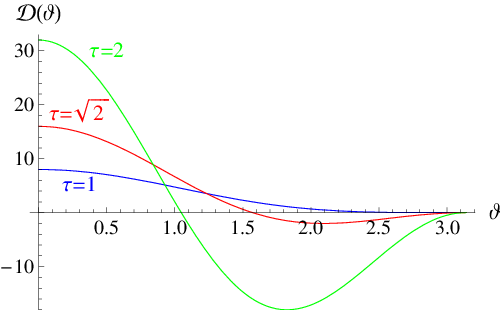
the function is positive for small and becomes negative if exceeds a certain value . Following Definition 1.3, two points and are timelike separated if and spacelike separated if .
Our action principle is to minimize the action (1.24) by varying the measure in the family of normalized Borel measures on the sphere. In order to solve this problem numerically, we approximate the minimizing measure by a weighted counting measure. Thus for any given integer , we choose points together with corresponding weights with
and introduce the measure by
| (4.1) |
where denotes the Dirac measure. Fixing different values of and seeking for numerical minimizers by varying both the points and the weights , we obtain the plots shown in Figure 2. It is surprising that for each fixed , the obtained minimal action no longer changes if is increased beyond a certain value . The numerics shows that if , some of the points coincide, so that the support of the minimizing measure never consists of more than points. Since this property remains true in the limit , our numerical analysis shows that the minimizing measure is discrete in the sense that its support consists of a finite number of points. Another interesting effect is that the action seems to favor symmetric configurations on the sphere. Namely, the most distinct local minima in Figure 2 correspond to configurations where the points lie on the vertices of Platonic solids. The analysis in [18] gives an explanation for this “discreteness” of the minimizing measure, as is made precise in the following theorem (for more general results in the same spirit see [18, Theorems 4.15 and 4.17]).

Theorem 4.1.
If , the support of every minimizing measure on the two-dimensional sphere is singular in the sense that it has empty interior.
Extrapolating to the general situation, this result indicates that our variational principle favors discrete over continuous configurations. Again interpreting as our space-time, this might correspond to a mechanism driven by our action principle which makes space-time discrete. Using a more graphic language, one could say that space-time “discretizes itself” on the Planck scale, thus avoiding the ultraviolet divergences of quantum field theory.
Another possible interpretation gives a connection to field quantization: Our model on the two-sphere involves one continuous parameter . If we allow to be varied while minimizing the action (as is indeed possible if we drop the constraint of prescribed eigenvalues), then the local minima of the action attained at discrete values of (like the configurations of the Platonic solids) are favored. Regarding as the amplitude of a “classical field”, our action principle gives rise to a “quantization” of this field, in the sense that the amplitude only takes discrete values.
The observed “discreteness” might also account for effects related to the wave-particle duality and the collapse of the wave function in the measurement process (for details see [13]).
5. The Correspondence to Quantum Field Theory and Gauge Theories
The correspondence to Minkowski space mentioned in Section 3.3 can also be used to analyze our action principle for interacting systems in the so-called continuum limit. We now outline a few ideas and constructions (for details see [6, Chapter 4], [9] and the survey article [14]). We first observe that the vacuum fermionic projector (1.5) is a solution of the Dirac equation . To introduce the interaction, we replace the free Dirac operator by a more general Dirac operator, which may in particular involve gauge potentials or a gravitational field. For simplicity, we here only consider an electromagnetic potential ,
| (5.1) |
Next, we introduce particles and anti-particles by occupying (suitably normalized) positive-energy states and removing states of the sea,
| (5.2) |
Using the so-called causal perturbation expansion and light-cone expansion, the fermionic projector can be introduced uniquely from (5.1) and (5.2).
It is important that our setting so far does not involve the field equations; in particular, the electromagnetic potential in the Dirac equation (5.1) does not need to satisfy the Maxwell equations. Instead, the field equations should be derived from our action principle (1.26). Indeed, analyzing the corresponding Euler-Lagrange equations, one finds that they are satisfied only if the potentials in the Dirac equation satisfy certain constraints. Some of these constraints are partial differential equations involving the potentials as well as the wave functions of the particles and anti-particles in (5.2). In [9], such field equations are analyzed in detail for a system involving an axial field. In order to keep the setting as simple as possible, we here consider the analogous field equation for the electromagnetic field
| (5.3) |
With (5.1) and (5.3), the interaction as described by the action principle (1.26) reduces in the continuum limit to the coupled Dirac-Maxwell equations. The many-fermion state is again described by the fermionic projector, which is built up of one-particle wave functions. The electromagnetic field merely is a classical bosonic field. Nevertheless, regarding (5.1) and (5.3) as a nonlinear hyperbolic system of partial differential equations and treating it perturbatively, one obtains all the Feynman diagrams which do not involve fermion loops. Taking into account that by exciting sea states we can describe pair creation and annihilation processes, we also get all diagrams involving fermion loops. In this way, we obtain agreement with perturbative quantum field theory (for details see [9, §8.4] and the references therein).
We finally remark that in the continuum limit, the freedom in choosing the spinor basis (1.17) can be described in the language of standard gauge theories. Namely, introducing a gauge-covariant derivative with gauge potentials (see for example [22]), the transformation (1.18) gives rise to the local gauge transformations
| (5.4) |
with . The difference to standard gauge theories is that the gauge group cannot be chosen arbitrarily, but it is determined to be the isometry group of the spin space. In the case of spin dimension two, the corresponding gauge group allows for a unified description of electrodynamics and general relativity (see [6, Section 5.1]). By choosing a higher spin dimension (see [6, Section 5.1]), one gets a larger gauge group. Our mathematical framework ensures that our action principle and thus also the continuum limit is gauge symmetric in the sense that the transformations (5.4) with map solutions of the equations of the continuum limit to each other. However, our action is not invariant under local transformations of the form (5.4) if is not unitary. An important example of such non-unitary transformations are chiral gauge transformations like
Thus chiral gauge transformations do not describe a gauge symmetry in the above sense. In the continuum limit, this leads to a mechanism which gives chiral gauge fields a rest mass (see [9, Section 8.5] and [14, Section 7]). Moreover, in systems of higher spin dimension, the presence of chiral gauge fields gives rise to a spontaneous breaking of the gauge symmetry, resulting in a smaller “effective” gauge group. As shown in [6, Chapters 6-8], these mechanisms make it possible to realize the gauge groups and couplings of the standard model.
Acknowledgments: We thank the referee for helpful suggestions on the manuscript.
References
- [1] H. Baum, Spinor structures and Dirac operators on pseudo-Riemannian manifolds, Bull. Polish Acad. Sci. Math. 33 (1985), no. 3-4, 165–171.
- [2] Y. Bernard and F. Finster, On the structure of minimizers of causal variational principles in the non-compact and equivariant settings, arXiv:1205.0403 [math-ph], Adv. Calc. Var. 7 (2014), no. 1, 27–57.
- [3] J. Bognár, Indefinite Inner Product Spaces, Springer-Verlag, New York, 1974, Ergebnisse der Mathematik und ihrer Grenzgebiete, Band 78.
- [4] L. Bombelli, J. Lee, D. Meyer, and R.D. Sorkin, Space-time as a causal set, Phys. Rev. Lett. 59 (1987), no. 5, 521–524.
- [5] F. Finster, Derivation of local gauge freedom from a measurement principle, arXiv:funct-an/9701002, Photon and Poincare Group (V. Dvoeglazov, ed.), Nova Science Publishers, 1999, pp. 315–325.
- [6] by same author, The Principle of the Fermionic Projector, hep-th/0001048, hep-th/0202059, hep-th/0210121, AMS/IP Studies in Advanced Mathematics, vol. 35, American Mathematical Society, Providence, RI, 2006.
- [7] by same author, Fermion systems in discrete space-time—outer symmetries and spontaneous symmetry breaking, arXiv:math-ph/0601039, Adv. Theor. Math. Phys. 11 (2007), no. 1, 91–146.
- [8] by same author, A variational principle in discrete space-time: Existence of minimizers, arXiv:math-ph/0503069, Calc. Var. Partial Differential Equations 29 (2007), no. 4, 431–453.
- [9] by same author, An action principle for an interacting fermion system and its analysis in the continuum limit, arXiv:0908.1542 [math-ph] (2009).
- [10] by same author, From discrete space-time to Minkowski space: Basic mechanisms, methods and perspectives, arXiv:0712.0685 [math-ph], Quantum Field Theory (B. Fauser, J. Tolksdorf, and E. Zeidler, eds.), Birkhäuser Verlag, 2009, pp. 235–259.
- [11] by same author, Causal variational principles on measure spaces, arXiv:0811.2666 [math-ph], J. Reine Angew. Math. 646 (2010), 141–194.
- [12] by same author, Entanglement and second quantization in the framework of the fermionic projector, arXiv:0911.0076 [math-ph], J. Phys. A: Math. Theor. 43 (2010), 395302.
- [13] by same author, The fermionic projector, entanglement, and the collapse of the wave function, arXiv:1011.2162 [quant-ph], J. Phys.: Conf. Ser. 306 (2011), 012024.
- [14] by same author, A formulation of quantum field theory realizing a sea of interacting Dirac particles, arXiv:0911.2102 [hep-th], Lett. Math. Phys. 97 (2011), no. 2, 165–183.
- [15] F. Finster and A. Grotz, A Lorentzian quantum geometry, arXiv:1107.2026 [math-ph], Adv. Theor. Math. Phys. 16 (2012), no. 4, 1197–1290.
- [16] F. Finster and M. Reintjes, A non-perturbative construction of the fermionic projector on globally hyperbolic manifolds I – Space-times of finite lifetime, arXiv:1301.5420 [math-ph] (2013).
- [17] by same author, A non-perturbative construction of the fermionic projector on globally hyperbolic manifolds II – Space-times of infinite lifetime, arXiv:1312.7209 [math-ph] (2013).
- [18] F. Finster and D. Schiefeneder, On the support of minimizers of causal variational principles, arXiv:1012.1589 [math-ph], Arch. Ration. Mech. Anal. 210 (2013), no. 2, 321–364.
- [19] F. Finster and J. Tolksdorf, Perturbative description of the fermionic projector: Normalization, causality and Furry’s theorem, arXiv:1401.4353 [math-ph], J. Math. Phys. 55 (2014), no. 5, 052301.
- [20] P.R. Halmos, Measure Theory, Springer, New York, 1974.
- [21] H.B. Lawson, Jr. and M.-L. Michelsohn, Spin Geometry, Princeton Mathematical Series, vol. 38, Princeton University Press, Princeton, NJ, 1989.
- [22] S. Pokorski, Gauge Field Theories, second ed., Cambridge Monographs on Mathematical Physics, Cambridge University Press, Cambridge, 2000.