Graver basis for an undirected graph and its application to testing the beta model of random graphs
Abstract
In this paper we give an explicit and algorithmic description of Graver basis for the toric ideal associated with a simple undirected graph and apply the basis for testing the beta model of random graphs by Markov chain Monte Carlo method.
Keywords and phrases: Markov basis, Markov chain Monte Carlo, Rasch model, toric ideal.
1 Introduction
Random graphs and their applications to the statistical modeling of complex networks have been attracting much interest in many fields, including statistical mechanics, ecology, biology and sociology (e.g. Newman [10], Goldenberg et al [6]). Statistical models for random graphs have been studied since Solomonoff and Rapoport [19] and Erdős and Rényi [5] introduced the Bernoulli random graph model. The beta model generalizes the Bernoulli model to a discrete exponential family with vertex degrees as sufficient statistics. The beta model was discussed by Holland and Leinhardt [8] in the directed case and by Park and Newman [15], Blitzstein and Diaconis [1] and Chatterjee et al [2] in the undirected case. The Rasch model [17], which is a standard model in the item response theory, is also interpreted as a beta model for undirected complete bipartite graphs. In this article we discuss the random sampling of graphs from the conditional distribution in the beta model when the vertex degrees are fixed.
In the context of social network the vertices of the graph represent individuals and their edges represent relationships between individuals. In the undirected case the graphs are sometimes restricted to be simple, i.e., no loops or multiple edges exist. The sample size for such cases is at most the number of edges of the graph and is often small. The goodness of fit of the model is usually assessed by large sample approximation of the distribution of a test statistic. When the sample size is not large enough, however, it is desirable to use a conditional test based on the exact distribution of a test statistic. For the general background on conditional tests and Markov bases, see Drton et al [4].
Random sampling of graphs with a given vertex degree sequence enables us to numerically evaluate the exact distribution of a test statistics for the beta model. Blitzstein and Diaconis [1] developed a sequential importance sampling algorithm for simple graphs which generates graphs through operations on vertex degree sequence. In this article we construct a Markov chain Monte Carlo algorithm for sampling graphs by using the Graver basis for the toric ideal arising from the underlying graph of the beta model.
A Markov basis [3] is often used for sampling from discrete exponential families. Algebraically a Markov basis for the underlying graph of the beta model is defined as a set of generators of the toric ideal arising from the underlying graph of the beta model. A set of graphs with a given vertex degree sequence is called a fiber for the underlying graph of the beta model. A Markov basis for the underlying graph of the beta model is also considered as a set of Markov transition operators connecting all elements of every fiber. Petrović et al [16] discussed some properties of the toric ideal arising from the model of [8] and provided Markov bases of the model for small directed graphs. Properties of toric ideals arising from a graph have been studied in a series of papers by Ohsugi and Hibi ([11], [12], [13]).
The Graver basis is the set of primitive binomials of the toric ideal. Applications of the Graver basis to integer programming are discussed in Onn [14]. Since the Graver basis is a superset of any minimal Markov basis, the Graver basis is also a Markov basis and therefore connects every fiber. When the graph is restricted to be simple, however, a Markov basis does not necessarily connect all elements of every fiber. A recent result by Hara and Takemura [7] implies that the set of square-free elements of the Graver basis connects all elements of every fiber of simple graphs with a given vertex degree sequence. Thus if we have the Graver basis, we can sample graphs from any fiber, with or without the restriction that graphs are simple, in such a way that every graph in the fiber is generated with positive probability.
In the sequential importance sampling algorithm of [1] the underlying graph for the model was assumed to be complete, i.e., all the edges have positive probability. In our approach we can allow that some edges are absent from the beginning (structural zero edges in the terminology of contingency table analysis), such as the bipartite graph for the case of the Rasch model. In fact the Graver basis for an arbitrary graph is obtained by restriction of the Graver basis for the complete graph to the existing edges of (cf. Proposition 4.13 of Sturmfels [20]). Moreover our algorithm can be applied not only for sampling simple graphs but also for sampling general undirected graphs without substantial adjustment. These are the advantages of the Graver basis.
The Graver basis for small graphs can be computed by a computer algebra system such as 4ti2 (4ti2 team [21]). For even moderate-sized graphs, however, it is difficult to compute the Graver basis via 4ti2 in a practical amount of time. In this article we first provide a complete description of the Graver basis for an undirected graph. In general the number of elements of the Graver basis is too large. So we construct an adaptive algorithm for sampling elements from the Graver basis, which is enough for constructing a connected Markov chain over any fiber. The recent paper of Reyes et al [18] discusses the Graver basis for an undirected graph and gives a characterization of the Graver basis. We give a new description of the Graver basis, which is more suitable for sampling elements from the Graver basis.
The organization of this paper is as follows. In Section 2 we give a brief review on some statistical models for random graphs and clarify the connection between the models and toric ideals arising from graphs. In Section 3 we provide an explicit description of the Graver basis for the toric ideal associated with an undirected graph. Section 4 gives an algorithm for random sampling of square-free elements of the Graver basis. In Section 5 we apply the proposed algorithm to some data sets and confirm that it works well in practice. We conclude the paper with some remarks in Section 6.
2 The beta model of random graphs
In this section we give a brief review of the beta model for undirected graphs according to Chatterjee et al [2].
Let be an undirected graph with vertices . Here we assume that has no loop. Let be the set of edges. For each edge , let a non-negative integer be the weight for and denote . is considered as an dimensional integer vector. We assume that an observed graph is generated by independent binomial distribution for each edge , i.e., with
Then the probability of is described as
| (1) |
The model (1) is called the beta model [2]. Note that if then the observed graph does not have an edge even if for the underlying graph .
This model was considered by many authors (e.g. Park and Newman [15], Blitzstein and Diaconis [1] and Chatterjee et al [2]). The model for random directed graphs by Holland and Leinhardt [8] can be interpreted as a generalization of the beta model. When is a complete bipartite graph, the beta model coincides with the Rasch model [17]. The many-facet Rasch model by Linacre [9], which is a multivariate version of the Rasch model, can be interpreted as a generalization of the beta model such that is a complete -partite graph.
Let be a degree sequence, i.e., for each vertex . Denote . The sufficient statistic for (1) is . Let denote the incidence matrix between vertices and edges of . Then it is easily seen that and are related as
A set of graphs (without restriction to be simple) with a given degree sequence is called a fiber for (or for the underlying graph ). An integer array of the same dimension as is called a move if . A move is written as the difference of its positive part and negative part as . Since , every move is written as the difference of two graphs in the same fiber. A finite set of moves is called a Markov basis for the incidence matrix if for every fiber any two graphs are mutually accessible by the moves in the set [3]. By adding or subtracting moves in a Markov basis, we can sample graphs from any fiber in such a way that every graph in the fiber is generated with positive probability. Note that in the beta model (1) is restricted as . We denote the subset of the fiber with this restriction as .
To assess the goodness of fit of the beta model we usually utilize a large sample approximation of the distribution of a test statistics. However, when ’s are not large enough, it is not appropriate to use the large sample approximation. Especially, as mentioned in Section 1, graphs are restricted to be simple () in some practical problems. For a simple graph, , , is either zero or one. A Markov basis for the incidence matrix guarantees the connectivity of every fiber if the restriction that graphs are simple is not imposed. Under the restriction, however, a Markov basis does not necessarily connect the subset of the fiber . For example, consider the beta model with the underlying graph in Figure 1 and for each edge . It can be shown that a set of all -cycles in is a Markov basis for the incidence matrix of . However and in Figure 1 are not mutually accessible by 4-cycles under the restriction that graphs are simple.

For a given , denotes the set of observed edges of . For two moves , the sum is called conformal if there is no cancellation of signs in , i.e., . The set of moves which can not be written as a conformal sum of two nonzero moves is called the Graver basis. The Graver basis is known to be a Markov basis [4, e.g.]. A move is square-free if the absolute values of its elements are or . By the same augment of Proposition 2.1 of Hara and Takemura [7], we can obtain the following proposition.
Proposition 1.
The Graver basis for the underlying graph of the beta model connects all elements of every fiber. Furthermore, the set of square-free moves of the Graver basis connects all elements of every fiber with the restriction of simple graphs.
Proof.
Let be two elements of the same fiber. The difference is written as a conformal sum of primitive moves:
| (2) |
where are elements of the Graver basis. Since there is no cancellation of signs on the right hand side, belongs to the same fiber for . Therefore the Graver basis connects all elements of every fiber.
Suppose for every in the setting of the beta model. It is easy to see that each is square-free in (2). It means that the set of square-free moves of the Graver basis connects all elements of every fiber with the restriction of simple graphs. ∎
Therefore it suffices to have the Graver basis to sample graphs from any fiber with or without the restriction that graphs are simple. In the next section we derive the Graver basis for the underlying graph of the beta model
3 Graver basis for an undirected graph
In this section we will give two characterizations of the Graver basis for an undirected graph. Theorem 1 in Section 3.2 is the main result of this paper which gives a necessary and sufficient condition for a element of the Graver basis as a sequence of vertices. Proposition 3, which is used for the proof of Theorem 1, gives a characterization of the Graver basis through recursive operations on the graph, which is of some independent interests.
3.1 Preliminaries
Let be a simple connected graph with and . A walk connecting and is a finite sequence of edges of the form
with . The length of the walk is the number of edges of the walk. An even (respectively odd) walk is a walk of even (respectively odd) length. A walk is closed if . A cycle is a closed walk with for every .
For a walk , let denote the set of vertices appearing in and let denote the set of edges appearing in . Furthermore let be the subgraph of , whose vertices and edges appear in the walk .
In order to describe known results on the toric ideal arising from an undirected graph , we give an algebraic definition of . Let be a polynomial ring in variables over . We will associate each edge with the monomial . Let be a polynomial ring in variables over and let be a homomorphism from to defined by . Then the toric ideal of the graph is defined as
A binomial is called primitive if there is no binomial , , such that and . The Graver basis of is the set of all primitive binomials belonging to and we denote it by . If we write the monomials as , then if and only if is a move. Furthermore is primitive if and only if and can not be written as a conformal sum of two nonzero moves.
For a given even closed walk we define a binomial as
An even closed walk is a proper subwalk of , if and hold for the binomial . Note that even if there is a proper subwalk of an even closed walk , dose not necessarily go along with , i.e., the edges of may not appear as consecutive edges of . An even closed walk is called primitive, if its binomial is primitive. Then the primitiveness of is equal to non-existence of a proper subwalk of .
A characterization of the primitive walks of graph , which gives a necessary condition for a binomial to be primitive, was given by Ohsugi and Hibi [12].
Proposition 2 ([12]).
Let be a finite connected graph. If is primitive, then we have where is one of the following even closed walks:
- (i)
is an even cycle of .
- (ii)
, where and are odd cycles of having exactly one common vertex.
- (iii)
, where and are odd cycles of having no common vertex and where and are walks of both of which contain a vertex of and a vertex of .
Every binomial in the first two cases is primitive but a binomial in the third case is not necessarily primitive.
3.2 Characterization of primitive walks
In this subsection we give a simple characterization of the primitive walks of a graph as sequences of vertices. Express an even closed walk as a sequence of vertices: , where . Let denote the number of times is visited in the walk before it returns to the vertex . Consider the following condition for the even closed walk .
Condition 1.
(i) for every vertex . (ii) For every vertex with and , , the closed walks and are odd walks with . (cf. Figure 2).
Remark 1.
Using Condition 1, we can characterize the Graver basis for a graph as follows.
Theorem 1.
A binomial is primitive if and only if there exists an even closed walk with satisfying Condition 1.
Remark 2.

Remark 3.
As mentioned in Section 1, there is another characterization of Graver basis in Theorem 3.1 of Reyes et al [18]. It also gives a necessary and sufficient condition for the primitiveness of even closed walks, by using some new graphical concepts such as “block” and “sink”. Our characterization in Theorem 1 gives a simpler description of Graver basis, because it does not need any new graphical concepts. Furthermore it is more convenient in the algorithmic viewpoint: When an even closed is given as a sequence of vertices or edges, we can easily determine if is primitive by checking directly Condition 1 without distinguishing any graphical objects.
Before proving Theorem 1, we state another characterization of primitive walks given in Proposition 3 below. In order to that, we need some more definitions on graphs. For a walk , let denote the weighted subgraph of where is the weight function defined by for each edge . For simplicity, we denote a weight (respectively ) by (respectively ) in our figures. For a vertex , we define two kinds of degrees of vertex :
is the usual degree of in . Note that the same weighted graph might correspond to two different even closed walks , i.e. . Given a weighted graph , we say that spans if and .
Now we define two operations, contraction and separation, on a weighted graph .
- •
Let be an edge with , whose removal from increases the number of connected components of the remaining subgraph. Contraction of is an operation as shown in Figure 3. That is, it first replaces by where consists of all edges of contained in , together with all edges , where is an edge of different from . Then, it defines by inversion of the signs of weights of edges belonging to the -side of .

Figure 3: Contraction. - •
Let be a vertex with , such that the removal of increases the number of connected components of the remaining subgraph and the positive side as well as the negative side of fit to one of three cases (a)–(c) (respectively to the sign reverse cases) in Figure 4. Separation of is an operation as shown in Figure 4. That is, it first deletes the vertex and all edges connected to on . Then, in the case of (a), it adds a new edge with weight . In the case of (b), it redefines and then contracts , where we assume that the contraction of is possible. In the case of (c), it redefines . We call this an edge with weight . The sign reverse cases are defined in the same way.

Figure 4: Separation.
Note that the separation is not defined for any vertex with , if fits to none of three cases (a)–(c) in Figure 4. The vertex in Figure 5 is such an example, because its positive side fits to none of three cases (a)–(c) in Figure 4.
Let insertion and binding be the reverse operations of contraction and separation, respectively. With these operations, consider the following condition for an even closed walk .
Condition 2.
(i) . Every vertex satisfies . For every vertex with , its removal from increases the number of connected components of the remaining subgraph. (ii) Let be a graph obtained by recursively applying contraction and separation of all possible edges and vertices in . Then each connected component of is an even cycle or an edge with weight 0.

Proposition 3.
For an even closed walk , the binomial is primitive if and only if satisfies Condition 2.
We establish some lemmas to prove Proposition 3. Our proof also shows that in Condition 2 does not depend on the order of application of contractions and separations excepting the sign inversion of weights of edges of each connected component in .
Lemma 1.
If is a primitive walk, satisfies (i) in Condition 2.
Proof.
Consider a vertex . Since is closed, is even. Furthermore, since is primitive, holds which implies that there is no cancellation in the calculation of weight on any edge. Then, a half of the weight is assigned as positive weights and other half is assigned as negative weights to the edges connected to on . Therefore . Now suppose . Consider that we start from a vertex along an edge with positive weight and go along the walk or its reverse until returning back to again for the first time. Since is primitive, we have to come back to along an edge with positive weight for the first time. Let us continue along or its reverse until returning back to . By the same reasoning, the last edge of this closed walk has a negative weight. This implies that this even closed walk becomes a proper subwalk of , a contradiction to the primitiveness of . Therefore is or .
To prove the remaining part, let be a vertex with and consider all closed walks on , where the edge starting from and the edge coming back to have positive weights. Let be the set of vertices other than which appear in one of these walks and is defined in the same way. Then holds. First, we show . Suppose that there exists a vertex . Then, as shown in Figure 6, there are two closed walks and . This implies that we can construct a proper subwalk of by the combination of , and , a contradiction to the primitiveness of . Therefore .

Second, suppose that the removal of the vertex from does not increase the number of connected components of the remaining subgraph. Then, there are vertices such that , because holds as shown above. Hence, as shown in Figure 7, an even closed walk is a proper subwalk of for appropriate , , which contradicts to the primitiveness of . Therefore the removal of from increases the number of connected components of the remaining subgraph.

∎
In the following four lemmas, we show that contraction, separation, and these inverse operations preserve the primitiveness of an even closed walk. The proofs of lemmas are postponed to Appendix.
Lemma 2.
Let an even closed walk be primitive and be the weighted graph which is obtained by a contraction for an edge with its weight on . Then any even closed walk spanning is primitive.
Lemma 3.
Let an even closed walk be primitive and be the weighted graphs obtained by the separation of a vertex . Then any even closed walks spanning are primitive or of length two with .
Lemma 4.
Let be a primitive walk and let be the weighted graph obtained by the insertion to with on . Then any even closed walk spanning is primitive.
Lemma 5.
Let each be a primitive walk or a closed walk with length two, and be the weighted subgraph obtained by binding of and . Then any even closed walk spanning is primitive.
Proof of Proposition 3.
Let be a primitive walk. From Lemma 1 satisfies (i) in Condition 2 and every edge with can be contracted. Furthermore, it is easy to see that every vertex with can be separated after recursively applying contractions of all possible edges. Therefore holds for every vertex on . From Lemmas 2 and 3, each even closed walk corresponding to the connected component of is primitive or of length two. Then, every connected component of is an even cycle or an edge with weight 0, because from Proposition 2 every primitive walk includes a vertex with if it is not an even cycle. Therefore, a primitive walk satisfies Condition 2. Conversely, suppose an even closed walk satisfies Condition 2. From Proposition 2 and Lemmas 4 and 5, is primitive. ∎
Proof of Theorem 1.
Let be a primitive walk. From Lemma 1, holds for each vertex and holds for each vertex with . By the primitiveness of , the closed walks and along are odd closed walks. Therefore satisfies Condition 1.
Conversely, let be an even closed walk with Condition 1. From Proposition 3, it suffices to show that satisfies Condition 2. The condition (i) in Condition 2 follows from Condition 1. Then, it is enough to confirm that satisfies the condition (ii) in Condition 2.
First, we claim that every edge with can be contracted and every vertex with and , i.e. , can be separated. The case of contraction is obvious from Condition 1. We confirm the case of separation. Consider the vertex in Figure 8.

If an edge dose not exist or exists with weight , it belongs to the case (a) or (b) in Figure 4, respectively. Let us consider the case that there exists an edge with weight and suppose that the vertex connects to more than three edges as shown in Figure 9.

Then, and appear in like or , because holds. This implies that is even as shown in Figure 10, which contradicts Condition 1. Hence the case with with weight belongs to (c) in Figure 4. Therefore the claim is confirmed.

Second, we verify that contraction and separation on preserve Condition 1. Consider the case of contraction of an edge . From Condition 1, such appear in as . The contraction of is equivalent to replacing by . This change causes the decrease of two edges from , and preserves Condition 1. The case of separation is checked in the same way.
4 Algorithm for generating elements of Graver basis
In this section we present an algorithm for generating elements randomly from the Graver basis for a simple undirected graph. As shown in Proposition 1, for testing the beta model of random graphs with , we only need square-free elements of the Graver basis. Therefore the restriction to square-free elements of our algorithm will be discussed in Remark 4. Theorem 1 guarantees the correctness of our algorithm.
We need some tools in order to construct an algorithm. Let be a weighted tree where is a weight function. For this weighted tree , let us consider the following condition.
Condition 3.
For each vertex , and .
With these tools, let us consider generating an element of the Graver basis for a simple undirected graph . For simplicity, first consider the case that that is complete. We call an edge with a cycle in for an even closed walk in this section. We will discuss later the case that is not complete. Let be a weighted tree satisfying Condition 3 and the following equation:
| (3) |
Then, we can construct a primitive walk in using as follows. First, we assign the set of vertices with for each vertex under the equation
and every vertex is assigned at most twice. Equation (3) guarantees that this assignment is possible. Second, we make cycles in by arbitrarily ordering the vertices . Then we make a subgraph of by taking the union of these cycles. Finally, we obtain a closed walk by choosing a root vertex from this subgraph and going around it. It is easy to see that this closed walk is primitive by Theorem 1.
Conversely we can construct a weighted tree with Condition 3 and (3) from each primitive walk. Let be a primitive walk. First, the vertex set is constructed by creating a vertex of for each cycle in . Second, the edge set is obtained by adding edge to for each pair of cycles in with . Then, we assign weight to each vertex .
Therefore, once we have a weighted tree with Condition 3 and (3), we can construct an element of the Graver basis for . Such a tree is constructed by the following algorithm.
Algorithm 1 (Algorithm for constructing an weighted tree).
Input : A complete graph .
Output : A weighted tree with Condition 3 and (3).
- 1.
Let be empty sets and .
- 2.
Add a root vertex to .
- 3.
Assign a weight from randomly.
- 4.
Grow by the following loop.
- (a)
For each vertex which is deepest from , add edges to and the endpoints () to , where the number is randomly decided under the following two conditions:
- •
.
- •
.
- •
- (b)
For each new vertex , assign a weight from randomly, where .
- (c)
Recompute and if , delete all new vertices and edges in the above (a) and break the loop.
- (d)
If the total number of new edges is equal to 0, break the loop.
- (e)
Return to (a).
- (a)
- 5.
If and is odd, change to or .
- 6.
If and has a leaf with even weight, subtract or add 1 to the weight.
- 7.
Output .
Algorithm 1 provides a simple algorithm for generating an element of Graver basis as follows.
Algorithm 2 (Algorithm for generating an element of Graver basis).
Since there is no restarts in Algorithm 2, it has a fixed worst case running time for a complete graph . In each step, the algorithm performs operations. Then it generates one element of the Graver basis for in time. A demonstration for the case of a complete graph with is shown in Figures 11 and 12. The output of this demonstration is a primitive walk with in Figure 12.


Remark 4.
For the case that an input graph is not complete, the elements of the Graver basis for can be generated by throwing away elements with supports not contained in (Proposition 4.13 of Sturmfels [20]). In fact this is the advantage of considering the Graver basis. The restriction for generation of square-free elements of the Graver basis can be realized by a slight modification in Algorithm 1. In fact, it suffices to change merely to in Step 3 and in (b) of Step 4 in Algorithm 1.
Remark 5.
Algorithm 2 allows us to uniformly sample graphs with the common degree sequence via Metropolis-Hastings algorithm with the Graver basis, with or without the restriction that graphs are simple. It is done by constructing a connected Markov chain of graphs with the common degree sequence. In each iteration, a primitive walk is randomly generated by Algorithm 2. If the primitive walk is applicable, a new sample graph with the same degree sequence is obtained by adding the primitive walk, otherwise the primitive walk is rejected. Note that Metropolis-Hastings algorithm does not require the uniformity of the distribution of generated primitive walks. As long as there is a positive probability of generating every element of the Graver basis, the Metropolis-Hastings algorithm realizes uniform sampling of graphs with the common degree sequence.
5 Numerical experiments
In this section we present numerical experiments with elements of the Graver basis computed by Algorithm 2 in Section 4. The implementation of Metropolis-Hastings algorithm with Algorithm 2 is done by Java 1.6.0 on Windows OS with Intel(R) Core(TM) i7-2829QM CPU@2.30GHz.
5.1 A simulation with a small graph
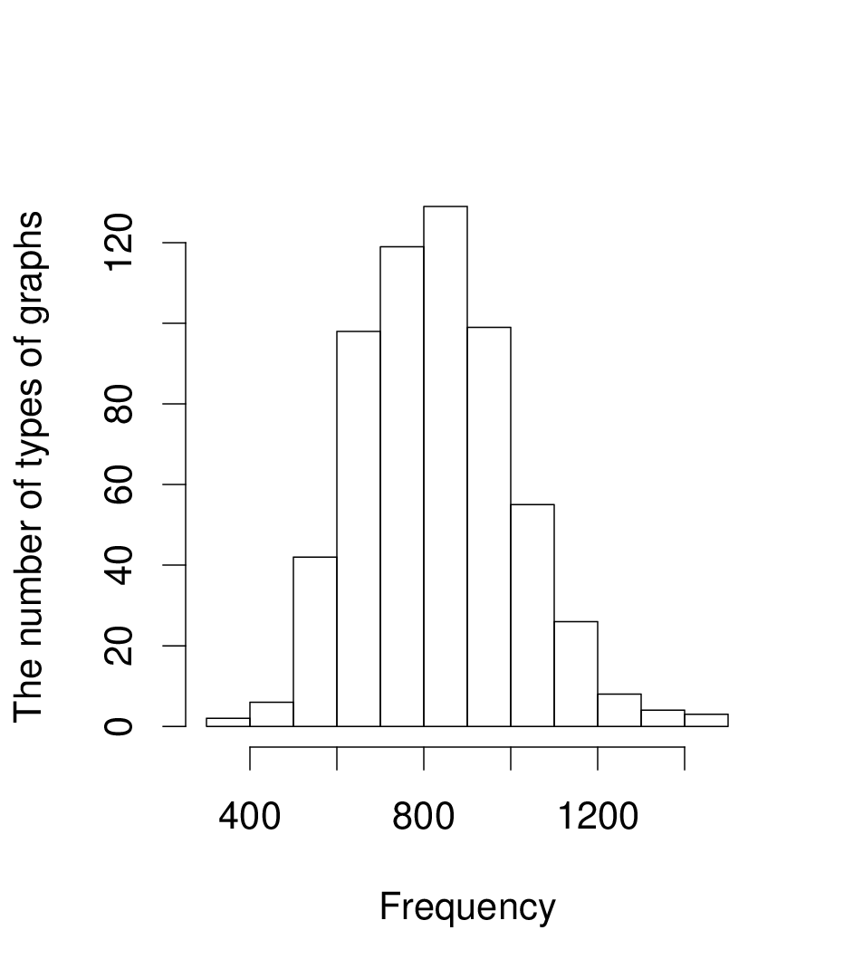
We run a Markov chain over the fiber containing a small graph in Figure 14. The underlying graph is assumed to be complete with eight vertices. By the Markov chain we sampled 510,000 graphs in the fiber, including 10,000 burn-in steps. The number of types of obtained graphs in our chain is 591. By enumeration we checked that 591 is actually the number of the elements of the fiber of . The histogram of this experiment is shown in Figure 14. The horizontal axis expresses the frequency of each type of graph and the vertical axis expresses the number of types. The mean of the number of appearances of each type is 829 and the standard deviation is 179. This experiment shows that the algorithm samples each element of the fiber almost uniformly.

5.2 The beta model for the food web data
We apply Algorithm 2 for testing of the real data, the observed food web of 36 types of organisms in the Chesapeake Bay during the summer. This data is available online at [22]. Blitzstein and Diaconis [1] analyzed essentially the same data set.

The graph of the data is shown in Figure 15. The vertices represent the types of organisms like blue crab, bacteria etc., and the edges represent the relationship of one preying upon the other. The degree sequence of is
Although there is a self loop at the vertex 19 in the observation, we ignored it for simplicity.
We set the beta model (1) in Section 2 with for each edge as the null hypothesis. Then the probability of is described as
| (5) |
Parameter is interpreted as the value of organism represented by the vertex as a food to other organisms. Then the beta model (5) implies that a vertex with large is likely to be connected to many edges. Let mean that can be expressed by (5) for a set of parameters . Consider now the statistical hypothesis testing problem
Starting from the graph in Figure 15, we construct a Markov chain of 10,100,000 graphs including 100,000 burn-in steps and compute the chi-square statistic of each graph as a test statistic. The running time of the calculation is 5 minutes and 4.8 seconds. Using the maximum likelihood estimator, the chi-square value of observed graph is 477 and the histogram of the estimated distribution of the chi-square values is shown in Figure 16. The approximate -value is 0.286. This value is not so small and there is no evidence against the beta model (5).

Next we consider some other characteristics of the observed graph and graphs obtained by the above Markov chain. We compute their clustering coefficient defined by Wattz and Strogatz [23] and also count the number of triangles (-cycles). For the observed graph , the values of clustering coefficient and the number of triangles are 0.447 and 101, respectively. For the sampled graphs, the histograms are obtained as in Figure 18 and 18 and their mean values are 0.436 and 92.4, respectively. The differences between the actual values and the means of sampled graphs are not large. It suggests that these statistics agree with the beta model (5).


As mentioned in Section 1 there are computer algebra systems such as 4ti2 (4ti2 team [21]) to compute the Graver basis. However the whole Graver basis is huge and difficult to compute even for a moderate-sized graph like the real data above. Algorithm 2, our adaptive algorithm, enables us to perform the Markov chain Monte Carlo method for such a moderate-sized graph.
6 Concluding remarks
In this paper we obtained a simple characterization of the Graver basis for toric ideals arising from undirected graphs. This Graver basis allows us to perform the conditional test of the beta model for arbitrary underlying graph. Our characterization allows us to construct an algorithm for sampling elements of the Graver basis, which is sufficient for performing the conditional test.
By numerical experiments we confirmed that our procedure works well in practice. We should mention that the sequential importance sampling method of Blitzstein and Diaconis [1] may work faster for the case of complete underlying graph.
If we allow multiple edges, then we do not need the Graver basis. A minimal Markov basis, which is often much smaller than the Graver basis, is sufficient for connectivity of Markov chains. Properties of Markov basis for the -model have been given in Petrović et al [16]. It is of interest to study properties of minimal Markov bases for undirected graphs, including the case of allowing self loops.
Acknowledgements We are very grateful to Hidefumi Ohsugi for valuable discussions. We also thank two referees for their valuable and constructive comments.
References
- [1] Blitzstein J, Diaconis P (2006) A sequential importance sampling algorithm for generating random graphs with prescribed degrees. Available at http://www.people.fas.harvard.edu/˜blitz/BlitzsteinDiaconisGraphAlgorithm.pdf, preprint
- [2] Chatterjee S, Diaconis P, Sly A (2010) Random graphs with a given degree sequence. arXiv:1005.1136v4
- [3] Diaconis P, Sturmfels B (1998) Algebraic algorithms for sampling from conditional distributions. Ann Statist 26(1):363–397
- [4] Drton M, Sturmfel B, Sullivant S (2008) Lectures on Algebraic Statistics. Oberwolfach Seminars, Birkhäuser Basel
- [5] Erdős P, Rényi A (1960) On the evolution of random graphs. Publications of the Mathematical Institute of the Hungarian Academy of Sciences 5:17–61
- [6] Goldenberg A, Zheng AX, Fienberg SE, Airoldi EM (2009) A survey of statistical network models. Foundations and Trends in Machine Learning 2:129–233
- [7] Hara H, Takemura A (2010) Connecting tables with zero-one entries by a subset of a markov basis. In: Algebraic Methods in Statistics and Probability II, Contemp. Math., vol 516, Amer. Math. Soc., Providence, RI, pp 199–213
- [8] Holland P, Leinhardt S (1981) An exponential family of probability distribution for directed graphs. J Amer Statist Soc 76(373):33–50
- [9] Linacre JM (1989) Many-facet Rasch Measurement. MESA Press, Chicago
- [10] Newman MEJ (2003) The structure and function of complex networks. SIAM Review 45:167–256
- [11] Ohsugi H, Hibi T (1999a) Koszul bipartite graphs. Adv in Appl Math 22(1):25–28
- [12] Ohsugi H, Hibi T (1999b) Toric ideals generated by quadratic binomials. J Algebra 218(2):509–527
- [13] Ohsugi H, Hibi T (2005) Indispensable binomials of finite graphs. J Algebra Appl 4(4):421–434
- [14] Onn S (2010) Nonlinear Discrete Optimization. Zurich Lectures in Advanced Mathematics, European Mathematical Society, DOI 10.4171/093
- [15] Park J, Newman MEJ (2004) The statistical mechanics of networks. Phys Rev E 70:066,117
- [16] Petrović S, Rinaldo A, Fienberg SE (2010) Algebraic statistics for a directed random graph model with reciprocation. In: Algebraic Methods in Statistics and Probability II, Contemp. Math., vol 516, Amer. Math. Soc., Providence, RI, pp 261–283
- [17] Rasch G (1980) Probabilistic Models for Some Intelligence and Attainment Tests. University of Chicago Press, Chicago
- [18] Reyes E, Tatakis C, Thoma A (2010) Minimal generators of toric ideals of graphs. arXiv:1002.2045v1
- [19] Solomonoff R, Rapoport A (1951) Connectivity of random nets. Bulletin of Mathematical Biophysics 13:107–117
- [20] Sturmfels B (1996) Gröbner Bases and Convex Polytopes, University Lecture Series, vol 8. American Mathematical Society, Providence, RI
- [21] 4ti2 team (2008) 4ti2—a software package for algebraic, geometric and combinatorial problems on linear spaces. Available at www.4ti2.de
- [22] Ulanowicz RE (2005) Ecosystem network analysis web page. URL http://www.cbl.umces.edu/˜ulan/ntwk/network.html
- [23] Wattz DJ, Strogatz SH (1998) Collective dynamics of small-world networks. Nature 393:440–442
Appendix A Proofs of Lemmas in Section 3.2
A.1 Proof of Lemma 2
The contraction of the edge with its weight on is possible from Lemma 1. We denote this edge by as shown in Figure 19.

Suppose is not primitive. Then there exists an proper subwalk of . If , is also a proper subwalk of , a contradiction to the primitiveness of . Then . However, a proper subwalk of is constructed by embedding into . Therefore, is primitive. ∎
A.2 Proof of Lemma 3
We consider the case that both positive and negative sides of correspond to (a) in Figure 4 and relevant edges are labeled as shown in Figure 20. Suppose is neither primitive nor of length two. Then there exists a proper subwalk of on .

If , is also a proper subwalk of , a contradiction to the primitiveness of . Then . Now is expressed as follows:
Then an even closed walk on
is a proper subwalk of . This contradicts the primitiveness of . Therefore is primitive or of length two. The cases of (b) and (c) in Figure 4 are shown in the same way. Note that it is easy to confirm the possibility of contraction after the step 1 in the case (b) from Lemma 1 and then the primitiveness is guaranteed by Lemma 2. By the same argument, the case of is confirmed. ∎
A.3 Proof of Lemma 4
Let be the new edge appearing through the insertion to as shown in Figure 21.

Suppose is not primitive. Then there exists a proper subwalk of . If , is contained in or . Then or its reverse becomes a proper subwalk of . This contradicts the primitiveness of . Hence . Then we can construct a proper subwalk of by removing from and reversing the weights of edges belonging to , a contradiction to the primitiveness of . Therefore, is primitive. ∎
A.4 Proof of Lemma 5
Let be the new vertex appearing through the binding. We consider the case that both positive and negative sides of correspond to (a) in Figure 4 and relevant edges are labeled as shown in Figure 22. Other cases are shown in the same way.

Suppose is not primitive. Then there exists a proper subwalk of . Here we choose a primitive walk as . If , is also a proper subwalk of or . Then . This implies that all four edges connected to appear in . Let us consider the separation of to . Then the resulting two weighted graphs are primitive from Lemma 3. Furthermore at least one of is a proper subwalk of , a contradiction to the primitiveness of . Therefore is primitive. ∎