跳到论文正文
W Papers独立论文阅读器 arXiv:1102.2250 论文正文 计算阅读时间 · 0%
引用这篇论文根据当前论文元数据生成,正式投稿前建议核对。


License: arXiv.org perpetual non-exclusive license
arXiv:1102.2250v1 [cs.IT] 10 Feb 2011

Modeling the pairwise key distribution scheme in the presence of unreliable links

Osman Yağan and Armand M. Makowski Affiliation: Department of Electrical and Computer Engineering
and the Institute for Systems Research
University of Maryland, College Park
College Park, Maryland 20742
oyagan@umd.edu, armand@isr.umd.edu
Abstract

We investigate the secure connectivity of wireless sensor networks under the pairwise key distribution scheme of Chan et al.. Unlike recent work which was carried out under the assumption of full visibility, here we assume a (simplified) communication model where unreliable wireless links are represented as on/off channels. We present conditions on how to scale the model parameters so that the network i) has no secure node which is isolated and ii) is securely connected, both with high probability when the number of sensor nodes becomes large. The results are given in the form of zero-one laws, and exhibit significant differences with corresponding results in the full visibility case. Through simulations these zero-one laws are shown to be valid also under a more realistic communication model, i.e., the disk model.

Keywords: Wireless sensor networks, Security, Key predistribution, Random graphs, Connectivity.

I Introduction

Wireless sensor networks (WSNs) are distributed collections of sensors with limited capabilities for computations and wireless communications. It is envisioned [1] that WSNs will be used in a wide range of applications areas such as healthcare (e.g. patient monitoring), military operations (e.g., battlefield surveillance) and homes (e.g., home automation and monitoring). These WSNs will often be deployed in hostile environments where communications can be monitored, and nodes are subject to capture and surreptitious use by an adversary. Under such circumstances, cryptographic protection will be needed to ensure secure communications, and to support functions such as sensor-capture detection, key revocation and sensor disabling.

Unfortunately, many security schemes developed for general network environments do not take into account the unique features of WSNs: Public key cryptography is not feasible computationally because of the severe limitations imposed on the physical memory and power consumption of the individual sensors. Traditional key exchange and distribution protocols are based on trusting third parties, and this makes them inadequate for large-scale WSNs whose topologies are unknown prior to deployment. We refer the reader to the papers [6, 11, 20] for discussions of the security challenges in WSN settings.

Random key predistribution schemes were introduced to address some of these difficulties. The idea of randomly assigning secure keys to sensor nodes prior to network deployment was first introduced by Eschenauer and Gligor [11]. Since then, many competing alternatives to the Eschenauer and Gligor (EG) scheme have been proposed; see [6] for a detailed survey of various key distribution schemes for WSNs. With so many schemes available, a basic question arises as to how they compare with each other. Answering this question passes through a good understanding of the properties and performance of the schemes under consideration, and this can be achieved in a number of ways. The approach we use here considers random graph models naturally induced by a given scheme, and then develops the scaling laws corresponding to desirable network properties, e.g., absence of secure nodes which are isolated, secure connectivity, etc. This is done with the aim of deriving guidelines to dimension the scheme, namely adjust its parameters so that these properties occur with high probability as the number of nodes becomes large.

To date, most of the efforts along these lines have been carried out under the assumption of full visibility according to which sensor nodes are all within communication range of each other; more on this later: Under this assumption, the EG scheme gives rise to a class of random graphs known as random key graphs; relevant results are available in the references [3, 8, 11, 18, 24]. The q-composite scheme [7], a simple variation of the EG scheme, was investigated by Bloznelis et al. [4] through an appropriate extension of the random key graph model. Recently, Yağan and Makowski have analyzed various random graphs induced by the random pairwise key predistribution scheme of Chan et al. [7]; see the conference papers [25, 26].

To be sure, the full visibility assumption does away with the wireless nature of the communication medium supporting WSNs. In return, this simplification makes it possible to focus on how randomization of the key distribution mechanism alone affects the establishment of a secure network in the best of circumstances, i..e., when there are no link failures. A common criticism of this line of work is that by disregarding the unreliability of the wireless links, the resulting dimensioning guidelines are likely to be too optimistic: In practice nodes will have fewer neighbors since some of the communication links may be impaired. As a result, the desired connectivity properties may not be achieved if dimensioning is done according to results derived under full visibility.

In this paper, in an attempt to go beyond full visibility, we revisit the pairwise key predistribution scheme of Chan et al. [7] under more realistic assumptions that account for the possibility that communication links between nodes may not be available – This could occur due to the presence of physical barriers between nodes or because of harsh environmental conditions severely impairing transmission. To study such situations, we introduce a simple communication model where channels are mutually independent, and are either on or off. An overall system model is then constructed by intersecting the random graph model of the pairwise key distribution scheme (under full visibility), with an Erdős-Rényi (ER) graph model [5]. For this new random graph structure, we establish zero-one laws for two basic (and related) graph properties, namely graph connectivity and the absence of isolated nodes, as the model parameters are scaled with the number of users – We identify the critical thresholds and show that they coincide. To the best of our knowledge, these full zero-one laws constitute the first complete analysis of a key distribution scheme under non-full visibility – Contrast this with the partial results by Yi et al. [28] for the absence of isolated nodes (under additional conditions) when the communication model is the disk model.

Although the communication model considered here may be deemed simplistic, it does permit a complete analysis of the issues of interest, with the results already yielding a number of interesting observations: The obtained zero-one laws differ significantly from the corresponding results in the full visibility case [25]. Thus, the communication model may have a significant impact on the dimensioning of the pairwise distribution algorithm, and this points to the need of possibly reevaluating guidelines developed under the full visibility assumption. Furthermore, simulations suggest that the zero-one laws obtained here for the on/off channel model may still be useful in dimensioning the pairwise scheme under the popular, and more realistic, disk model [12].

We also compare the results established here with well-known zero-one laws for ER graphs [5]. In particular, we show that the connectivity behavior of the model studied here does not in general resemble that of the ER graphs. The picture is somewhat more subtle for the results also imply that if the channel is very poor, the model studied here indeed behaves like an ER graph as far as connectivity is concerned. The comparison with ER graphs is particularly relevant to the analysis of key distribution schemes for WSNs: Indeed, connectivity results for ER graphs have often been used in the dimensioning and evaluation of key distribution schemes, e.g., see the papers by Eschenauer and Gligor [11], Chan et al. [7] and Hwang and Kim [13]. There it is a common practice to assume that the random graph induced by the particular key distribution scheme behaves like an ER graph (although it is not strictly speaking an ER graph). As pointed out by Di Pietro et al. [8] such an assumption is made without any formal justification, and subsequent efforts to confirm its validity have remained limited to this date: The EG scheme has been analyzed by a number of authors [3, 8, 18, 24], and as a result of these efforts it is now known that the ER assumption does yield the correct results for both the absence of isolated nodes and connectivity under the assumption of full visibility. On the other hand the recent paper [25] shows that the ER assumption is not valid for the pairwise key distribution of Chan et al. [7]; see Section V-A for details.

The rest of the paper is organized as follows: In Section II, we give precise definitions and implementation details of the pairwise scheme of Chan et al. while Section III is devoted to describing the model of interest. The main results of the paper, namely Theorem IV.1 and Theorem IV.2, are presented in Section IV with an extensive discussion given in Section V. The remaining sections, namely Sections VI through XIII, are devoted to establishing the main results of the paper.

A word on notation and conventions in use: All limiting statements, including asymptotic equivalences, are understood with nn going to infinity. The random variables (rvs) under consideration are all defined on the same probability triple (Ω,ℱ,ℙ)(\Omega,{\cal F},\mathbb{P}). Probabilistic statements are made with respect to this probability measure ℙ\mathbb{P}, and we denote the corresponding expectation operator by 𝔼\mathbb{E}. Also, we use the notation =s​t=_{st} to indicate distributional equality. The indicator function of an event EE is denoted by 𝟏​[E]{\bf 1}\left[E\right]. For any discrete set SS we write |S||S| for its cardinality. Also, for any pair of events EE and FF we have

𝟏​[E∪F]=𝟏​[E]+𝟏​[F]−𝟏​[E∩F].{\bf 1}\left[E\cup F\right]={\bf 1}\left[E\right]+{\bf 1}\left[F\right]-{\bf 1}\left[E\cap F\right]. (1)

II Implementing pairwise key distribution schemes

Interest in the random pairwise key predistribution scheme of Chan et al. [7] stems from the following advantages over the EG scheme: (i) Even if some nodes are captured, the secrecy of the remaining nodes is perfectly preserved; (ii) Unlike earlier schemes, this pairwise scheme enables both node-to-node authentication and quorum-based revocation.

As in the conference papers [25, 26], we parametrize the pairwise key distribution scheme by two positive integers nn and KK such that K<nK<n. There are nn nodes, labelled i=1,…,ni=1,\ldots,n, with unique ids Id1,…,Idn{\rm Id}_{1},\ldots,{\rm Id}_{n}. Write 𝒩:={1,…​n}{\cal N}:=\{1,\ldots n\} and set 𝒩−i:=𝒩−{i}{\cal N}_{-i}:={\cal N}-\{i\} for each i=1,…,ni=1,\ldots,n. With node ii we associate a subset Γn,i\Gamma_{n,i} of nodes selected at random from 𝒩−i{\cal N}_{-i} – We say that each of the nodes in Γn,i\Gamma_{n,i} is paired to node ii. Thus, for any subset A⊆𝒩−iA\subseteq{\cal N}_{-i}, we require

ℙ[Γn,i=A]={(n−1K)−1if |A|=K0otherwise.{\mathbb{P}}\left[{\Gamma_{n,i}=A}\right]=\left\{\begin{array}[]{ll}{{n-1}\choose{K}}^{-1}&\mbox{if $|A|=K$}\\ &\\ 0&\mbox{otherwise.}\end{array}\right.

The selection of Γn,i\Gamma_{n,i} is done uniformly amongst all subsets of 𝒩−i{\cal N}_{-i} which are of size exactly KK. The rvs Γn,1,…,Γn,n\Gamma_{n,1},\ldots,\Gamma_{n,n} are assumed to be mutually independent so that

ℙ[Γn,i=Ai,i=1,…,n]=∏i=1nℙ[Γn,i=Ai]{\mathbb{P}}\left[{\Gamma_{n,i}=A_{i},\ i=1,\ldots,n}\right]=\prod_{i=1}^{n}{\mathbb{P}}\left[{\Gamma_{n,i}=A_{i}}\right]

for arbitrary A1,…,AnA_{1},\ldots,A_{n} subsets of 𝒩−1,…,𝒩−n{\cal N}_{-1},\ldots,{\cal N}_{-n}, respectively.

Once this offline random pairing has been created, we construct the key rings Σn,1,…,Σn,n\Sigma_{n,1},\ldots,\Sigma_{n,n}, one for each node, as follows: Assumed available is a collection of n​KnK distinct cryptographic keys {ωi|ℓ,i=1,…,n;ℓ=1,…,K}\{\omega_{i|\ell},\ i=1,\ldots,n;\ \ell=1,\ldots,K\}. Fix i=1,…,ni=1,\ldots,n and let ℓn,i:Γn,i→{1,…,K}\ell_{n,i}:\Gamma_{n,i}\rightarrow\{1,\ldots,K\} denote a labeling of Γn,i\Gamma_{n,i}. For each node jj in Γn,i\Gamma_{n,i} paired to ii, the cryptographic key ωi|ℓn,i​(j)\omega_{i|\ell_{n,i}(j)} is associated with jj. For instance, if the random set Γn,i\Gamma_{n,i} is realized as {j1,…,jK}\{j_{1},\ldots,j_{K}\} with 1≤j1<…<jK≤n1\leq j_{1}<\ldots<j_{K}\leq n, then an obvious labeling consists in ℓn,i​(jk)=k\ell_{n,i}(j_{k})=k for each k=1,…,Kk=1,\ldots,K with key ωi|k\omega_{i|k} associated with node jkj_{k}. Of course other labeling are possible, e.g., according to decreasing labels or according to a random permutation. Finally, the pairwise key ωn,i​j⋆=[Idi​|Idj|​ωi|ℓn,i​(j)]\omega^{\star}_{n,ij}=[{\rm Id}_{i}|{\rm Id}_{j}|\omega_{i|\ell_{n,i}(j)}] is constructed and inserted in the memory modules of both nodes ii and jj. The key ωn,i​j⋆\omega^{\star}_{n,ij} is assigned exclusively to the pair of nodes ii and jj, hence the terminology pairwise distribution scheme. The key ring Σn,i\Sigma_{n,i} of node ii is the set

Σn,i:={ωn,i​j⋆,j∈Γn,i}∪{ωn,j​i⋆,i∈Γn,j}.\Sigma_{n,i}:=\{\omega^{\star}_{n,ij},\ j\in\Gamma_{n,i}\}\cup\{\omega^{\star}_{n,ji},\ i\in\Gamma_{n,j}\}. (2)

If two nodes, say ii and jj, are within communication range of each other, then they can establish a secure link if at least one of the events i∈Γn,ji\in\Gamma_{n,j} or j∈Γn,jj\in\Gamma_{n,j} is taking place. Both events can take place, in which case the memory modules of node ii and jj both contain the distinct keys ωn,i​j⋆\omega^{\star}_{n,ij} and ωn,j​i⋆\omega^{\star}_{n,ji}. Finally, it is plain by construction that this scheme supports node-to-node authentication.

III The model

Under full visibility, this pairwise distribution scheme naturally gives rise to the following class of random graphs: With n=2,3,…n=2,3,\ldots and positive integer K<nK<n, we say that the distinct nodes ii and jj are K-adjacent, written i∼Kji\sim_{K}j, if and only if they have at least one key in common in their key rings, namely

i∼KjiffΣn,i∩Σn,j≠∅.i\sim_{K}j\quad\mbox{iff}\quad\Sigma_{n,i}\cap\Sigma_{n,j}\neq\emptyset. (3)

Let ℍ⁡(n,K)\mathbb{H}(n;K) denote the undirected random graph on the vertex set {1,…,n}\{1,\ldots,n\} induced by the adjacency notion (3); this corresponds to modelling the pairwise distribution scheme under full visibility. We have

ℙ[i∼Kj]=λn(K){\mathbb{P}}\left[{i\sim_{K}j}\right]=\lambda_{n}(K) (4)

where λn​(K)\lambda_{n}(K) is the link assignment probability in ℍ⁡(n,K)\mathbb{H}(n;K) given by

λn​(K)\displaystyle\lambda_{n}(K) =\displaystyle= 1−(1−Kn−1)2\displaystyle 1-\left(1-\frac{K}{n-1}\right)^{2} (5)
=\displaystyle= 2​Kn−1−(Kn−1)2.\displaystyle\frac{2K}{n-1}-\left(\frac{K}{n-1}\right)^{2}.

As mentioned earlier, in this paper we seek to account for the possibility that communication links between nodes may not be available. To study such situations, we assume a communication model that consists of independent channels each of which can be either on or off. Thus, with pp in (0,1)(0,1), let {Bi​j(p),1≤i<j≤n}\{B_{ij}(p),1\leq i<j\leq n\} denote i.i.d. {0,1}\{0,1\}-valued rvs with success probability pp. The channel between nodes ii and jj is available (resp. up) with probability pp and unavailable (resp. down) with the complementary probability 1−p1-p.

Distinct nodes ii and jj are said to be B-adjacent, written i∼Bji\sim_{B}j, if Bi​j​(p)=1B_{ij}(p)=1. The notion of B-adjacency defines the standard ER graph 𝔾⁡(n,p)\mathbb{G}(n;p) on the vertex set {1,…,n}\{1,\ldots,n\}. Obviously,

ℙ[i∼j]B=p.{\mathbb{P}}\left[{i\sim j}\right]_{B}=p.

The random graph model studied here is obtained by intersecting the random pairwise graph ℍ⁡(n,K)\mathbb{H}(n;K) with the ER graph 𝔾⁡(n,p)\mathbb{G}(n;p). More precisely, the distinct nodes ii and jj are said to be adjacent, written i∼ji\sim j, if and only they are both K-adjacent and B-adjacent, namely

i∼jiffΣn,i∩Σn,j≠∅andBi​j​(p)=1.i\sim j\quad\mbox{iff}\quad\begin{array}[]{c}\Sigma_{n,i}\cap\Sigma_{n,j}\neq\emptyset\\ \mbox{and}\\ B_{ij}(p)=1.\\ \end{array} (6)

The resulting undirected random graph defined on the vertex set {1,…,n}\{1,\ldots,n\} through this notion of adjacency is denoted ℍ∩𝔾⁡(n,K,p)\mathbb{H\cap G}(n;K,p).

Throughout the collections of rvs {Γn,1,…,Γn,n}\{\Gamma_{n,1},\ldots,\Gamma_{n,n}\} and {Bi​j(p),1≤i<j≤n}\{B_{ij}(p),1\leq i<j\leq n\} are assumed to be independent, in which case the edge occurrence probability in ℍ∩𝔾⁡(n,K,p)\mathbb{H\cap G}(n;K,p) is given by

ℙ[i∼j]=p⋅ℙ[i∼Kj]=pλn(K).{\mathbb{P}}\left[{i\sim j}\right]=p\cdot{\mathbb{P}}\left[{i\sim_{K}j}\right]=p\lambda_{n}(K). (7)

IV The results

To fix the terminology, we refer to any mapping K:ℕ0→ℕ0K:\mathbb{N}_{0}\rightarrow\mathbb{N}_{0} as a scaling (for random pairwise graphs) provided it satisfies the natural conditions

Kn<n,n=1,2,….K_{n}<n,\quad n=1,2,\ldots. (8)

Similarly, any mapping p:ℕ0→(0,1)p:\mathbb{N}_{0}\rightarrow(0,1) defines a scaling for ER graphs.

To lighten the notation we often group the parameters KK and pp into the ordered pair θ≡(K,p)\theta\equiv(K,p). Hence, a mapping θ:ℕ0→ℕ0×(0,1)\theta:\mathbb{N}_{0}\rightarrow\mathbb{N}_{0}\times(0,1) defines a scaling for the intersection graph ℍ∩𝔾⁡(n,θ)\mathbb{H\cap G}(n;\theta) provided the condition (8) holds on the first component.

The results will be expressed in terms of the threshold function τ:[0,1]→[0,1]\tau:[0,1]\rightarrow[0,1] defined by

τ⁡(p)={1if p=021−log⁡(1−p)pif 0<p<10if p=1.\tau(p)=\left\{\begin{array}[]{lll}1&\mbox{if~ $p=0$}\\ &\\ \frac{2}{1-\frac{\log(1-p)}{p}}&\mbox{if~$0<p<1$}\\ &\\ 0&\mbox{if~$p=1$.}\end{array}\right. (9)

It is easy to check that this threshold function is continuous on its entire domain of definition; see Figure 3.

IV-A Absence of isolated nodes

The first result gives a zero-one law for the absence of isolated nodes.

Theorem IV.1

Consider scalings K:ℕ0→ℕ0K:\mathbb{N}_{0}\rightarrow\mathbb{N}_{0} and p:ℕ0→(0,1)p:\mathbb{N}_{0}\rightarrow(0,1) such that

pn(2Kn−Kn2n−1)∼clogn,n=1,2,…p_{n}\left(2K_{n}-\frac{K_{n}^{2}}{n-1}\right)\sim c\log n,\quad n=1,2,\ldots (10)

for some c>0c>0. If limn→∞pn=p⋆\lim_{n\to\infty}p_{n}=p^{\star} for some p⋆p^{\star} in [0,1][0,1], then we have

limn→∞ℙ⁡[ℍ∩𝔾⁡(n,θn)​contains no isolated nodes]\displaystyle\lim_{n\rightarrow\infty}{\mathbb{P}}\left[{\begin{array}[]{c}\mathbb{H\cap G}(n;\theta_{n})~\mbox{contains}\\ \mbox{~no~isolated~nodes}\\ \end{array}}\right]
=\displaystyle= {0if c<τ⁡(p⋆)1if c>τ⁡(p⋆).\displaystyle\left\{\begin{array}[]{ll}0&\mbox{if~ $c<\tau(p^{\star})$}\\ &\\ 1&\mbox{if~$c>\tau(p^{\star})$.}\end{array}\right.

The condition (10) on the scaling ℕ0→(0,1)×ℕ0\mathbb{N}_{0}\rightarrow(0,1)\times\mathbb{N}_{0} will often be used in the equivalent form

pn(2Kn−Kn2n−1)=cnlogn,n=1,2,…p_{n}\left(2K_{n}-\frac{K_{n}^{2}}{n-1}\right)=c_{n}\log n,\quad n=1,2,\ldots (18)

with the sequence c:ℕ0→ℝ+c:\mathbb{N}_{0}\rightarrow\mathbb{R}_{+} satisfying limn→∞cn=c\lim_{n\rightarrow\infty}c_{n}=c.

IV-B Connectivity

An analog of Theorem IV.1 also holds for the property of graph connectivity.

Theorem IV.2

Consider scalings K:ℕ0→ℕ0K:\mathbb{N}_{0}\rightarrow\mathbb{N}_{0} and p:ℕ0→(0,1)p:\mathbb{N}_{0}\rightarrow(0,1) such that (10) holds for some c>0c>0. If limn→∞pn=p⋆\lim_{n\to\infty}p_{n}=p^{\star} for some p⋆p^{\star} in [0,1][0,1], then we have

limn→∞ℙ⁡[ℍ∩𝔾⁡(n,θn)​ is connected]\displaystyle\lim_{n\rightarrow\infty}{\mathbb{P}}\left[{\mathbb{H\cap G}(n;\theta_{n})~\mbox{ is connected}}\right]
=\displaystyle= {0if c<τ⁡(p⋆)1if c>τ⁡(p⋆)\displaystyle\left\{\begin{array}[]{ll}0&\mbox{if~ $c<\tau(p^{\star})$}\\ &\\ 1&\mbox{if~$c>\tau(p^{\star})$}\end{array}\right.

where the threshold τ⁡(p⋆)\tau(p^{\star}) is given by (9).

Comparing Theorem IV.2 with Theorem IV.1, we see that the class of random graphs studied here provides one more instance where the zero-one laws for absence of isolated nodes and connectivity coincide, viz. ER graphs [5], random geometric graphs [19] or random key graphs [3, 18, 24].

A case of particular interest arises when p⋆>0p^{\star}>0 since requiring (10) now amounts to

(2​Kn−Kn2n−1)∼cp⋆​log⁡n\left(2K_{n}-\frac{K_{n}^{2}}{n-1}\right)\sim~\frac{c}{p^{\star}}\log n (23)

for some c>0c>0. Any scaling K:ℕ0→ℕ0K:\mathbb{N}_{0}\rightarrow\mathbb{N}_{0} which behaves like (23) must necessarily satisfy Kn=o⁡(n)K_{n}=o(n), and it is easy to see that requiring (10) is equivalent to

Kn∼t​log⁡nK_{n}\sim~t\log n (24)

for some t>0t>0 with cc and tt related by t=c2​p⋆t=\frac{c}{2p^{\star}}. With this reparametrization, Theorem IV.1 and Theorem IV.2 can be summarized in the following simpler form:

Theorem IV.3

Consider scalings K:ℕ0→ℕ0K:\mathbb{N}_{0}\rightarrow\mathbb{N}_{0} and p:ℕ0→(0,1)p:\mathbb{N}_{0}\rightarrow(0,1) such that limn→∞pn=p⋆>0\lim_{n\to\infty}p_{n}=p^{\star}>0. Under the condition (24) for some t>0t>0, we have

limn→∞ℙ⁡[ℍ∩𝔾⁡(n,θn)​contains no isolated nodes]\displaystyle\lim_{n\rightarrow\infty}{\mathbb{P}}\left[{\mathbb{H\cap G}(n;\theta_{n})~\mbox{contains~no~isolated~nodes}}\right]
=\displaystyle= limn→∞ℙ⁡[ℍ∩𝔾⁡(n,θn)​ is connected]\displaystyle\lim_{n\rightarrow\infty}{\mathbb{P}}\left[{\mathbb{H\cap G}(n;\theta_{n})~\mbox{ is connected}}\right]
=\displaystyle= {0if t<τ^​(p⋆)1if t>τ^​(p⋆)\displaystyle\left\{\begin{array}[]{ll}0&\mbox{if~ $t<\widehat{\tau}(p^{\star})$}\\ &\\ 1&\mbox{if~ $t>\widehat{\tau}(p^{\star})$}\end{array}\right.

where we have set

τ^​(p):=τ⁡(p)2​p=1p−log⁡(1−p),0<p<1.\widehat{\tau}(p):=\frac{\tau(p)}{2p}=\frac{1}{p-\log(1-p)},\quad 0<p<1. (29)

This alternate formulation is particularly relevant for the case pn=p⋆p_{n}=p^{\star} (in (0,1)(0,1)) for all n=1,2,…n=1,2,\ldots, which captures situations when channel conditions are not affected by the number of users. Such simplifications do not occur in the more realistic case p⋆=0p^{\star}=0 which corresponds to the situation where channel conditions are indeed influenced by the number of users in the system – The more users in the network, the more likely they will experience interferences from other users.

We now present numerical results that verify (IV.3). In all the simulations, we fix the number of nodes at n=200n=200. We consider the channel parameters p=0.2p=0.2, p=0.4p=0.4, p=0.6p=0.6, p=0.8p=0.8, and p=1p=1 (the full visibility case), while varying the parameter KK from 11 to 2525. For each parameter pair (K,p)(K,p), we generate 500500 independent samples of the graph ℍ∩𝔾⁡(n,K,p)\mathbb{H}\cap\mathbb{G}(n;K,p) and count the number of times (out of a possible 500) that the obtained graphs i) have no isolated nodes and ii) are connected. Dividing the counts by 500500, we obtain the (empirical) probabilities for the events of interest. The results for connectivity are depicted in Figure 1, where the curve fitting tool of MATLAB is used. It is easy to check that for each value of p≠1p\neq 1, the connectivity threshold matches the prescription (IV.3), namely K=τ^​(p)​log⁡nK=\widehat{\tau}(p)\log n. It is also seen that, if the channel is poor, i.e., if pp is close to zero, then the required value for KK to ensure connectivity can be much larger than the one in the full visibility case p=1p=1. The results regarding the absence of node isolation are depicted in Figure 2. For each value of p≠1p\neq 1, Figure 2 is indistinguishable from Figure 1, with the difference between the estimated probabilities of graph connectivity and absence of isolated nodes being quite small, in agreement with (IV.3).

Refer to caption
Fig. 1: Probability that ℍ∩𝔾⁡(n,K,p)\mathbb{H}\cap\mathbb{G}(n;K,p) is connected as a function of KK for p=0.2p=0.2, p=0.4p=0.4, p=0.6p=0.6, p=0.8p=0.8 and p=1p=1 with n=200n=200.
Refer to caption
Fig. 2: Probability that ℍ∩𝔾⁡(n,K,p)\mathbb{H}\cap\mathbb{G}(n;K,p) has no isolated nodes as a function of KK for p=0.2p=0.2, p=0.4p=0.4, p=0.6p=0.6, p=0.8p=0.8 and p=1p=1 with n=200n=200. This figure clearly resembles Figure 1 for all p≠1p\neq 1.

V Discussion and comments

V-A Comparing with the full-visibility case

At this point the reader may wonder as to what form would Theorem IV.2 take in the context of full visibility– In the setting developed here this corresponds to p=1p=1 so that ℍ∩𝔾⁡(n,θ)\mathbb{H\cap G}(n;\theta) coincides with ℍ⁡(n,K)\mathbb{H}(n;K); see the curve for p=1p=1 in Figure 1). Relevant results for this case were obtained recently by the authors in [25].

Theorem V.1

For any KK a positive integer, it holds that

limn→∞ℙ[ℍ(n;K) is connected]={0if K=11if K≥2.\lim_{n\rightarrow\infty}{\mathbb{P}}\left[{\mathbb{H}(n;K)~\mbox{ is connected}}\right]=\left\{\begin{array}[]{ll}0&\mbox{if~ $K=1$}\\ &\\ 1&\mbox{if~$K\geq 2$.}\end{array}\right.

The case where the parameter KK is scaled with nn is an easy corollary of Theorem V.1.

Corollary V.2

For any scaling K:ℕ0→ℕ0K:\mathbb{N}_{0}\rightarrow\mathbb{N}_{0} such that Kn≥2K_{n}\geq 2 for all nn sufficiently large, we have the one-law

limn→∞ℙ[ℍ(n;Kn) is connected]=1.\lim_{n\rightarrow\infty}{\mathbb{P}}\left[{\mathbb{H}(n;K_{n})~\mbox{ is connected}}\right]=1.

Each node in ℍ⁡(n,K)\mathbb{H}(n;K) has degree at least KK, so that no node is ever isolated in ℍ⁡(n,K)\mathbb{H}(n;K). This is in sharp contrast with the model studied here, as reflected by the full zero-one law for node isolation given in Theorem IV.1.

Theorem V.1 and its Corollary V.2 together show that very small values of KK suffice to ensure asymptotically almost sure (a.a.s.) connectivity of the random graph ℍ⁡(n,K)\mathbb{H}(n;K). However, these two results cannot be recovered from Theorem IV.2 whose zero-one laws are derived under the assumption pn<1p_{n}<1 for all n=1,2,…n=1,2,\ldots. Furthermore, even if the scaling p:ℕ0→(0,1)p:\mathbb{N}_{0}\rightarrow(0,1) were to satisfy limn→∞pn=1\lim_{n\rightarrow\infty}p_{n}=1, only the one-laws in Theorem 29 remain since τ⁡(p⋆)=0\tau(p^{\star})=0 (and τ^​(p⋆)=0\widehat{\tau}(p^{\star})=0) at p⋆=1p^{\star}=1. Although this might perhaps be expected given the aforementioned absence of isolated nodes in ℍ⁡(n,K)\mathbb{H}(n;K), the one-laws for both the absence of isolated nodes and graph connectivity in ℍ∩𝔾⁡(n,θ)\mathbb{H}\cap\mathbb{G}(n;\theta) still require conditions on the behavior of the scaling K:ℕ0→ℕ0K:\mathbb{N}_{0}\rightarrow\mathbb{N}_{0}, namely (24) (whereas Corollary V.2 does not).

V-B Comparing ℍ∩𝔾⁡(n,θ)\mathbb{H\cap G}(n;\theta) with ER graphs

In the original paper of Chan et al. [7] (as in the reference [13]), the connectivity analysis of the pairwise scheme was based on ER graphs [5] – It was assumed that the random graph induced by the pairwise scheme under a communication model (taken mostly to be the disk model [12]) behaves like an ER graph; similar assumptions have been made in [11, 13] when discussing the connectivity of the EG scheme. However, this assumption was made without any formal justification. Recently we have shown that the full visibility model ℍ⁡(n,K)\mathbb{H}(n;K) has major differences with an ER graph. For instance, the edge assignments are (negatively) correlated in ℍ⁡(n,K)\mathbb{H}(n;K) while independent in ER graphs; see [25] for a detailed discussion on the differences of ℍ⁡(n,K)\mathbb{H}(n;K) and 𝔾⁡(n,p)\mathbb{G}(n;p). It is easy to verify that the edge assignments in ℍ∩𝔾⁡(n,θ)\mathbb{H\cap G}(n;\theta) are also negatively correlated; see Section IX. Therefore, the models ℍ⁡(n,K)\mathbb{H}(n;K) and ℍ∩𝔾⁡(n,θ)\mathbb{H\cap G}(n;\theta) cannot be equated with an ER graph, and the results obtained in [25] and in this paper are not mere consequences of classical results for ER graphs.

However, formal similarities do exist between ℍ∩𝔾⁡(n,θ)\mathbb{H\cap G}(n;\theta) and ER graphs. Recall the following well-known zero-one law for ER graphs: For any scaling p:ℕ0→[0,1]p:\mathbb{N}_{0}\rightarrow[0,1] satisfying

pn∼c​log⁡nnp_{n}\sim c~\frac{\log n}{n}

for some c>0c>0, it holds that

limn→∞ℙ⁡[𝔾⁡(n,pn)​is connected]={0if c<11if c>1.\lim_{n\rightarrow\infty}{\mathbb{P}}\left[{\mathbb{G}(n;p_{n})~\mbox{\rm is~connected}}\right]=\left\{\begin{array}[]{ll}0&\mbox{if~ $c<1$}\\ &\\ 1&\mbox{if~ $c>1$.}\end{array}\right.

On the other hand, the condition (10) can be rephrased more compactly as

pn​λn​(Kn)∼c​log⁡nn,c>0p_{n}\lambda_{n}(K_{n})\sim c~\frac{\log n}{n},\qquad c>0

with the results (IV.1) and (IV.2) unchanged. Hence, in both ER graphs and ℍ∩𝔾⁡(n,θ)\mathbb{H\cap G}(n;\theta), the zero-one laws can be expressed as a comparison of the probability of link assignment against the critical scaling log⁡nn\frac{\log n}{n}; this is also the case for random geometric graphs [19], and random key graphs [3, 18, 24]. But the condition c>τ⁡(p⋆)c>\tau(p^{\star}) that ensures a.a.s. connectivity in ℍ∩𝔾⁡(n,θ)\mathbb{H}\cap\mathbb{G}(n;\theta) is not the same as the condition c>1c>1 for a.a.s. connectivity in ER graphs; see Figure 3. Thus, the connectivity behavior of the model ℍ∩𝔾⁡(n,θ)\mathbb{H}\cap\mathbb{G}(n;\theta) is in general different from that in an ER graph, and a “transfer” of the connectivity results from ER graphs cannot be taken for granted. Yet, the comparison becomes intricate when the channel is poor: The connectivity behaviors of the two models do match in the practically relevant case (for WSNs) limn→∞pn=0\lim_{n\to\infty}p_{n}=0 since τ⁡(0)=1\tau(0)=1.

Refer to caption
Fig. 3: τ⁡(p)\tau(p) vs pp. Clearly τ⁡(p⋆)=1\tau(p^{\star})=1 only if limn→∞pn=p⋆=0\lim_{n\to\infty}p_{n}=p^{\star}=0.

V-C A more realistic communication model

Refer to caption
Fig. 4: Probability that ℍ∩𝔾⁡(n,K,ρ)\mathbb{H}\cap\mathbb{G}(n;K,\rho) is connected as a function of KK. The number of nodes is set to n=200n=200 and ρ\rho is given by π​ρ2=p\pi\rho^{2}=p.

One possible extension of the work presented here would be to consider a more realistic communication model; e.g., the popular disk model [12] which takes into account the geographical positions of the sensor nodes. For instance, assume that the nodes are distributed over a bounded region 𝒟\mathcal{D} of the plane. According to the disk model, nodes ii and jj located at 𝒙𝒊\boldsymbol{x_{i}} and 𝒙𝒋\boldsymbol{x_{j}}, respectively, in 𝒟\mathcal{D} are able to communicate if

∥𝒙𝒊−𝒙𝒋∥<ρ\parallel\boldsymbol{x_{i}}-\boldsymbol{x_{j}}\parallel<\rho (30)

where ρ>0\rho>0 is called the transmission range. When the node locations are independently and randomly distributed over the region 𝒟\mathcal{D}, the graph induced under the condition (30) is known as a random geometric graph [19], thereafter denoted 𝔾⁡(n,ρ)\mathbb{G}(n;\rho).

Under the disk model, studying the pairwise scheme of Chan et al. amounts to analyzing the intersection of ℍ⁡(n,K)\mathbb{H}(n;K) and 𝔾⁡(n,ρ)\mathbb{G}(n;\rho), say ℍ∩𝔾⁡(n,K,ρ)\mathbb{H\cap G}(n;K,\rho). A direct analysis of this model seems to be very challenging; see below for more on this. However, limited simulations already suggest that the zero-one laws obtained here for ℍ∩𝔾⁡(n,K,p)\mathbb{H\cap G}(n;K,p) have an analog for the model ℍ∩𝔾⁡(n,K,ρ)\mathbb{H\cap G}(n;K,\rho). To verify this, consider 200200 nodes distributed uniformly and independently over a folded unit square [0,1]2[0,1]^{2} with toroidal (continuous) boundary conditions. Since there are no border effects, it is easy to check that

ℙ[∥𝒙𝒊−𝒙𝒋∥<ρ]=πρ2,i≠j,i,j=1,2,…,n.{\mathbb{P}}\left[{\>\parallel\boldsymbol{x_{i}}-\boldsymbol{x_{j}}\parallel<\rho\>}\right]=\pi\rho^{2},\quad i\neq j,\>\>i,j=1,2,\ldots,n.

whenever ρ<0.5\rho<0.5. We match the two communication models 𝔾⁡(n,p)\mathbb{G}(n;p) and 𝔾⁡(n,ρ)\mathbb{G}(n;\rho) by requiring π​ρ2=p\pi\rho^{2}=p. Then, we use the same procedure that produced Figure 1 to obtain the empirical probability that ℍ∩𝔾⁡(n,K,ρ)\mathbb{H\cap G}(n;K,\rho) is connected for various values of KK and pp. The results are depicted in Figure 4 whose resemblance with Figure 1 suggests that the connectivity behaviors of the models ℍ∩𝔾⁡(n,K,p)\mathbb{H\cap G}(n;K,p) and ℍ∩𝔾⁡(n,K,ρ)\mathbb{H\cap G}(n;K,\rho) are quite similar. This raises the possibility that the results obtained here for the on/off communication model can also be used for dimensioning the pairwise scheme under the disk model.

A complete analysis of ℍ∩𝔾⁡(n,K,ρ)\mathbb{H\cap G}(n;K,\rho) is likely to be very challenging given the difficulties already encountered in the analysis of similar problems. For example, the intersection of random geometric graphs with ER graphs was considered in [2, 28]. Although zero-one laws for graph connectivity are available for each component random graph, the results for the intersection model in [2, 28] were limited only to the absence of isolated nodes; the connectivity problem is still open for that model. Yi et al. [28] also consider the intersection of random key graphs with random geometric graphs, but these results are again limited to the property of node isolation. To the best of our knowledge, Theorem IV.2 reported here constitutes the only zero-one law for graph connectivity in a model formed by intersecting multiple random graphs! (Except of course the trivial case where an ER graph intersects another ER graph.)

V-D Intersection of random graphs

Refer to caption
Fig. 5: An instantiation of ER graph 𝔾⁡(n,p)\mathbb{G}(n;p) with n=50n=50 and p=0.2p=0.2.– The graph is connected.
Refer to caption
Fig. 6: An instantiation of ℍ⁡(n,K)\mathbb{H}(n;K) with n=50n=50 and K=5K=5.– The graph is connected.
Refer to caption
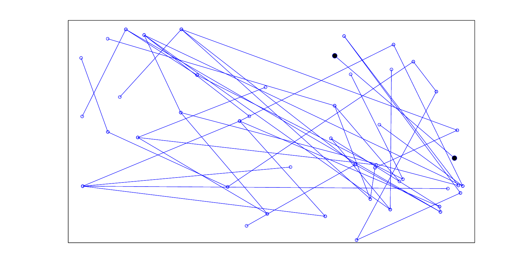
Fig. 7: The intersection ℍ∩𝔾⁡(n,θ)\mathbb{H\cap G}(n;\theta) of the graphs in Figure 5 and Figure 6 – The graph is disconnected as the marked nodes form a component!

When using random graph models to study networks, situations arise where the notion of adjacency between nodes reflects multiple constraints. This can be so even when dealing with networks other than WSNs. As was the case here, such circumstances call for studying models which are constructed by taking the intersection of multiple random graphs. However, as pointed out earlier, the availability of results for each component model does not necessarily imply the availability of results for the intersection of these models; see the examples provided in the previous section.

Figures 5-7 can help better understand the relevant issues as to why this is so: Figure 5 provides a sample of an ER graph 𝔾⁡(n,p)\mathbb{G}(n,p) with n=200n=200 and p=0.2p=0.2. As would be expected from the classical results, the obtained graph is very densely connected. Similarly, Figure 6 provides a sample of the pairwise random graph ℍ⁡(n,K)\mathbb{H}(n;K) with n=200n=200 and K=5K=5. In line with Theorem V.1, the obtained graph is connected. On the other hand, the graph formed by intersecting these graphs turn out to be disconnected as shown in Figure 7.

To drive this point further, consider the constant parameter case for the models ℍ⁡(n,K)\mathbb{H}(n;K) and 𝔾⁡(n,p)\mathbb{G}(n;p), a case which cannot be recovered from either Theorem IV.1 or Theorem IV.2. Nevertheless, Theorem V.1 yields

limn→∞ℙ[ℍ(n;K) is connected]=1,K≥2\lim_{n\rightarrow\infty}{\mathbb{P}}\left[{\mathbb{H}(n;K)~\mbox{ is connected}}\right]=1,\quad K\geq 2

while it well known [5] that

limn→∞ℙ[𝔾(n;p) is connected]=1.0<p<1.\lim_{n\rightarrow\infty}{\mathbb{P}}\left[{\mathbb{G}(n;p)~\mbox{ is connected}}\right]=1.\quad 0<p<1.

However, it can be shown that

limn→∞ℙ⁡[ℍ∩𝔾⁡(n,θ)​contains no isolated nodes]=0\lim_{n\rightarrow\infty}{\mathbb{P}}\left[{\mathbb{H\cap G}(n;\theta)~\mbox{contains}\mbox{~no~isolated~nodes}}\right]=0 (31)

whence

limn→∞ℙ⁡[ℍ∩𝔾⁡(n,θ)​is connected]=0\lim_{n\rightarrow\infty}{\mathbb{P}}\left[{\mathbb{H\cap G}(n;\theta)~\mbox{is connected}}\right]=0 (32)

for the same ranges of values for pp and KK; for details see the discussion at the end of Section X. This clearly provides a non-trivial example (one that is not for an ER intersecting an ER graph) where the intersection of two random graphs is indeed a.a.s. not connected although each of the components is a.a.s. connected.

VI A proof of Theorem IV.1

We prove Theorem IV.1 by the method of first and second moments [14, p. 55] applied to the total number of isolated nodes in ℍ∩𝔾⁡(n,θ)\mathbb{H\cap G}(n;\theta). First some notation: Fix n=2,3,…n=2,3,\ldots and consider θ=(K,p)\theta=(K,p) with pp in (0,1)(0,1) and positive integer KK such that K<nK<n. With

χn,i​(θ):=𝟏​[Node​i​is​isolated​in​ℍ∩𝔾⁡(n,θ)]\chi_{n,i}(\theta):={\bf 1}\left[{\rm Node~}i~{\rm is~isolated~in~}\mathbb{H\cap G}(n;\theta)\right]

for each i=1,…,ni=1,\ldots,n, the number of isolated nodes in ℍ∩𝔾⁡(n,θ)\mathbb{H\cap G}(n;\theta) is simply given by

In​(θ):=∑i=1nχn,i​(θ).I_{n}(\theta):=\sum_{i=1}^{n}\chi_{n,i}(\theta).

The random graph ℍ∩𝔾⁡(n,θ)\mathbb{H\cap G}(n;\theta) has no isolated nodes if and only if In​(θ)=0I_{n}(\theta)=0.

The method of first moment [14, Eqn (3.10), p. 55] relies on the well-known bound

1−𝔼[In(θ)]≤ℙ[In(θ)=0]1-{\mathbb{E}}\left[{I_{n}(\theta)}\right]\leq{\mathbb{P}}\left[{I_{n}(\theta)=0}\right] (33)

while the method of second moment [14, Remark 3.1, p. 55] has its starting point in the inequality

ℙ[In(θ)=0]≤1−𝔼​[In​(θ)]2𝔼⁡[In​(θ)2].{\mathbb{P}}\left[{I_{n}(\theta)=0}\right]\leq 1-\frac{{\mathbb{E}}\left[{I_{n}(\theta)}\right]^{2}}{{\mathbb{E}}\left[{I_{n}(\theta)^{2}}\right]}. (34)

The rvs χn,1​(θ),…,χn,n​(θ)\chi_{n,1}(\theta),\ldots,\chi_{n,n}(\theta) being exchangeable, we find

𝔼⁡[In​(θ)]=n​𝔼​[χn,1​(θ)]{\mathbb{E}}\left[{I_{n}(\theta)}\right]=n{\mathbb{E}}\left[{\chi_{n,1}(\theta)}\right] (35)

and

𝔼⁡[In​(θ)2]=n​𝔼​[χn,1​(θ)]+n⁡(n−1)​𝔼​[χn,1​(θ)​χn,2​(θ)]\displaystyle{\mathbb{E}}\left[{I_{n}(\theta)^{2}}\right]=n{\mathbb{E}}\left[{\chi_{n,1}(\theta)}\right]+n(n-1){\mathbb{E}}\left[{\chi_{n,1}(\theta)\chi_{n,2}(\theta)}\right]

by the binary nature of the rvs involved. It then follows that

𝔼⁡[In​(θ)2]𝔼​[In​(θ)]2\displaystyle\frac{{\mathbb{E}}\left[{I_{n}(\theta)^{2}}\right]}{{\mathbb{E}}\left[{I_{n}(\theta)}\right]^{2}} =\displaystyle= 1n​𝔼​[χn,1​(θ)]\displaystyle\frac{1}{n{\mathbb{E}}\left[{\chi_{n,1}(\theta)}\right]} (36)
+n−1n⋅𝔼⁡[χn,1​(θ)​χn,2​(θ)](𝔼⁡[χn,1​(θ)])2.\displaystyle+\frac{n-1}{n}\cdot\frac{{\mathbb{E}}\left[{\chi_{n,1}(\theta)\chi_{n,2}(\theta)}\right]}{\left({\mathbb{E}}\left[{\chi_{n,1}(\theta)}\right]\right)^{2}}.

From (33) and (35) we see that the one-law limn→∞ℙ[In(θn)=0]=1\lim_{n\to\infty}{\mathbb{P}}\left[{I_{n}(\theta_{n})=0}\right]=1 will be established if we show that

limn→∞n​𝔼​[χn,1​(θn)]=0.\lim_{n\to\infty}n{\mathbb{E}}\left[{\chi_{n,1}(\theta_{n})}\right]=0. (37)

It is also plain from (34) and (VI) that the zero-law limn→∞ℙ[In(θn)=0]=0\lim_{n\to\infty}{\mathbb{P}}\left[{I_{n}(\theta_{n})=0}\right]=0 holds if

limn→∞n​𝔼​[χn,1​(θn)]=∞\lim_{n\to\infty}n{\mathbb{E}}\left[{\chi_{n,1}(\theta_{n})}\right]=\infty (38)

and

lim supn→∞(𝔼⁡[χn,1​(θn)​χn,2​(θn)](𝔼⁡[χn,1​(θn)])2)≤1.\limsup_{n\to\infty}\left(\frac{{\mathbb{E}}\left[{\chi_{n,1}(\theta_{n})\chi_{n,2}(\theta_{n})}\right]}{\left({\mathbb{E}}\left[{\chi_{n,1}(\theta_{n})}\right]\right)^{2}}\right)\leq 1. (39)

The proof of Theorem IV.1 passes through the next two technical propositions which establish (37), (38) and (39) under the appropriate conditions on the scaling θ:ℕ0→ℕ0×(0,1)\theta:\mathbb{N}_{0}\rightarrow\mathbb{N}_{0}\times(0,1).

Proposition VI.1

Consider scalings K:ℕ0→ℕ0K:\mathbb{N}_{0}\rightarrow\mathbb{N}_{0} and p:ℕ0→(0,1)p:\mathbb{N}_{0}\rightarrow(0,1) such that (10) holds for some c>0c>0. Assume also that limn→∞pn=p⋆\lim_{n\to\infty}p_{n}=p^{\star} exists. Then, we have

limn→∞n​𝔼​[χn,1​(θn)]={0if c>τ⁡(p⋆)∞if c<τ⁡(p⋆)\lim_{n\rightarrow\infty}n{\mathbb{E}}\left[{\chi_{n,1}(\theta_{n})}\right]=\left\{\begin{array}[]{ll}0&\mbox{if~ $c>\tau(p^{\star})$}\\ &\\ \infty&\mbox{if~$c<\tau(p^{\star})$}\end{array}\right. (40)

where the threshold τ⁡(p⋆)\tau(p^{\star}) is given by (9).

A proof of Proposition VI.1 is given in Section VIII.

Proposition VI.2

Consider scalings K:ℕ0→ℕ0K:\mathbb{N}_{0}\rightarrow\mathbb{N}_{0} and p:ℕ0→(0,1)p:\mathbb{N}_{0}\rightarrow(0,1) such that (10) holds for some c>0c>0. Assume also that limn→∞pn=p⋆\lim_{n\to\infty}p_{n}=p^{\star} exists. Then, we have (39) whenever p⋆<1p^{\star}<1.

A proof of Proposition VI.2 can be found in Section X. To complete the proof of Theorem IV.1, pick a scaling θ:ℕ0→ℕ0×(0,1)\theta:\mathbb{N}_{0}\rightarrow\mathbb{N}_{0}\times(0,1) such that (10) holds for some c>0c>0 and limn→∞pn=p⋆\lim_{n\to\infty}p_{n}=p^{\star} exists. Under the condition c>τ⁡(p⋆)c>\tau(p^{\star}) we get (37) from Proposition VI.1, and the one-law limn→∞ℙ[In(θn)=0]=1\lim_{n\to\infty}{\mathbb{P}}\left[{I_{n}(\theta_{n})=0}\right]=1 follows. Next, assume that c<τ⁡(p⋆)c<\tau(p^{\star}) – This case is possible only if p⋆<1p^{\star}<1 since τ⁡(1)=0\tau(1)=0 as seen at (9). When p⋆<1p^{\star}<1, we obtain (38) and (39) with the help of Propositions VI.1 and VI.2, respectively. The conclusion limn→∞ℙ[In(θn)=0]=0\lim_{n\to\infty}{\mathbb{P}}\left[{I_{n}(\theta_{n})=0}\right]=0 is now immediate.

VII A preparatory result

Fix n=2,3,…n=2,3,\ldots and consider θ=(K,p)\theta=(K,p) with pp in (0,1)(0,1) and positive integer KK such that K<nK<n. Under the enforced assumptions, for all i=1,…,ni=1,\ldots,n, we easily see that

𝔼⁡[χn,i​(θ)]=𝔼⁡[(1−p)Dn,i]{\mathbb{E}}\left[{\chi_{n,i}(\theta)}\right]={\mathbb{E}}\left[{(1-p)^{D_{n,i}}}\right] (41)

where Dn,iD_{n,i} denotes the degree of node ii in ℍ⁡(n,K)\mathbb{H}(n;K). Note that

Dn,i\displaystyle D_{n,i} =\displaystyle= K+∑j=1,j∉Γn,i∪{i}n𝟏[i∈Γn,j].\displaystyle K+\sum_{j=1,j\notin\Gamma_{n,i}\cup\{i\}}^{n}{\bf 1}\left[i\in\Gamma_{n,j}\right]. (42)

By independence, since

|{j=1,…,n:j∉Γn,i∪{i}}|=n−K−1,|\{j=1,\ldots,n:\ j\notin\Gamma_{n,i}\cup\{i\}\}|=n-K-1,

the second term in (42) is a binomial rv with n−K−1n-K-1 trials and success probability given by

ℙ[i∈Γn,j]=(n−2K−1)(n−1K)=Kn−1,{\mathbb{P}}\left[{i\in\Gamma_{n,j}}\right]=\frac{{{n-2}\choose{K-1}}}{{{n-1}\choose{K}}}=\frac{K}{n-1}, (43)

whence

𝔼⁡[χn,i​(θ)]=(1−p)K⋅(1−p​Kn−1)n−K−1.{\mathbb{E}}\left[{\chi_{n,i}(\theta)}\right]=\left(1-p\right)^{K}\cdot\left(1-\frac{pK}{n-1}\right)^{n-K-1}. (44)

The proof of Proposition VI.1 uses a somewhat simpler form of the expression (44) which we develop next.

Lemma VII.1

Consider scalings K:ℕ0→ℕ0K:\mathbb{N}_{0}\rightarrow\mathbb{N}_{0} and p:ℕ0→(0,1)p:\mathbb{N}_{0}\rightarrow(0,1) such that (10) holds for some c>0c>0. It holds that

n​𝔼​[χn,1​(θn)]=eαn+o⁡(1)n=1,2,…n{\mathbb{E}}\left[{\chi_{n,1}(\theta_{n})}\right]=e^{\alpha_{n}+o(1)}\quad n=1,2,\ldots (45)

with

αn:=(1−cn)​log⁡n+Kn​(pn+log⁡(1−pn))\alpha_{n}:=(1-c_{n})\log n+K_{n}(p_{n}+\log(1-p_{n})) (46)

where the sequence c:ℕ0→ℝc:\mathbb{N}_{0}\rightarrow\mathbb{R} is the one appearing in the form (18) of the condition (10).

In what follows we make use of the decomposition

log⁡(1−x)=−x−Ψ⁡(x),0≤x<1\log(1-x)=-x-\Psi(x),\quad 0\leq x<1 (47)

with

Ψ⁡(x):=∫0xt1−t​𝑑t\Psi(x):=\int_{0}^{x}\frac{t}{1-t}dt

on that range. Note that

limx↓0Ψ⁡(x)x2=12.\lim_{x\downarrow 0}\frac{\Psi(x)}{x^{2}}=\frac{1}{2}.

Proof. Consider a scaling θ:ℕ0→ℕ0×(0,1)\theta:\mathbb{N}_{0}\rightarrow\mathbb{N}_{0}\times(0,1) such that (10) holds for some c>0c>0 and assume the existence of the limit limn→∞pn=p⋆\lim_{n\to\infty}p_{n}=p^{\star}. Replacing θ\theta by θn\theta_{n} in (44) for each n=2,3,…n=2,3,\ldots we get

n​𝔼​[χn,1​(θn)]=eβnn{\mathbb{E}}\left[{\chi_{n,1}(\theta_{n})}\right]=e^{\beta_{n}} (48)

with βn\beta_{n} given by

βn=log⁡n+Kn​log⁡(1−pn)−γn\beta_{n}=\log n+K_{n}\log(1-p_{n})-\gamma_{n}

with

γn:=−(n−Kn−1)​log⁡(1−pn​Knn−1).\gamma_{n}:=-(n-K_{n}-1)\log\left(1-\frac{p_{n}K_{n}}{n-1}\right).

The decomposition (47) now yields

γn\displaystyle\gamma_{n} :⁣=\displaystyle:= (n−Kn−1)​(pn​Knn−1+Ψ⁡(pn​Knn−1))\displaystyle(n-K_{n}-1)\left(\frac{p_{n}K_{n}}{n-1}+\Psi\left(\frac{p_{n}K_{n}}{n-1}\right)\right)
=\displaystyle= (1−Knn−1)​Kn​pn+(n−Kn−1)​Ψ​(pn​Knn−1)\displaystyle\left(1-\frac{K_{n}}{n-1}\right)K_{n}p_{n}+(n-K_{n}-1)\Psi\left(\frac{p_{n}K_{n}}{n-1}\right)
=\displaystyle= −Kn​pn+(2−Knn−1)​Kn​pn\displaystyle-K_{n}p_{n}+\left(2-\frac{K_{n}}{n-1}\right)K_{n}p_{n}
+(n−Kn−1)​Ψ​(pn​Knn−1)\displaystyle\quad\quad+(n-K_{n}-1)\Psi\left(\frac{p_{n}K_{n}}{n-1}\right)
=\displaystyle= −Kn​pn+cn​log⁡n+(n−Kn−1)​Ψ​(pn​Knn−1)\displaystyle-K_{n}p_{n}+c_{n}\log n+(n-K_{n}-1)\Psi\left(\frac{p_{n}K_{n}}{n-1}\right)

where the last step used the form (18) of the condition (10) on the scaling. Reporting this calculation into the expression for βn\beta_{n} we find

βn=αn−(n−Kn−1)​Ψ​(pn​Knn−1).\beta_{n}=\alpha_{n}-(n-K_{n}-1)\Psi\left(\frac{p_{n}K_{n}}{n-1}\right).

Lemma VII.1 will be established if we show that

limn→∞(n−Kn−1)​Ψ​(pn​Knn−1)=0.\lim_{n\rightarrow\infty}(n-K_{n}-1)\Psi\left(\frac{p_{n}K_{n}}{n-1}\right)=0. (49)

To that end, for each n=2,3,…n=2,3,\ldots we note that

pn​Kn≤pn​(2​Kn−Kn2n−1)≤2​pn​Knp_{n}K_{n}\leq p_{n}\left(2K_{n}-\frac{K_{n}^{2}}{n-1}\right)\leq 2p_{n}K_{n}

since Kn<nK_{n}<n. The condition (18) implies

cn2​log⁡n≤pn​Kn≤cn​log⁡n,\frac{c_{n}}{2}\log n\leq p_{n}K_{n}\leq c_{n}\log n, (50)

and it is now plain that

limn→∞pn​Knn−1=0andlimn→∞(n−Kn−1)​pn2​Kn2(n−1)2=0.\lim_{n\to\infty}\frac{p_{n}K_{n}}{n-1}=0\quad\mbox{and}\quad\lim_{n\to\infty}(n-K_{n}-1)\frac{p_{n}^{2}K_{n}^{2}}{(n-1)^{2}}=0.

Invoking the behavior of Ψ⁡(x)\Psi(x) at x=0x=0 mentioned earlier, we conclude from these facts that

limn→∞((n−Kn−1)​pn2​Kn2(n−1)2)​(Ψ⁡(pn​Knn−1)(pn​Knn−1)2)=0.\lim_{n\to\infty}\left((n-K_{n}-1)\frac{p_{n}^{2}K_{n}^{2}}{(n-1)^{2}}\right)\left(\frac{\Psi\left(\frac{p_{n}K_{n}}{n-1}\right)}{\left(\frac{p_{n}K_{n}}{n-1}\right)^{2}}\right)=0. (51)

This establishes (49) and the proof of Lemma VII.1 is completed.  

VIII A proof of Proposition VI.1

In view of Lemma VII.1, Proposition VI.1 will be established if we show

limn→∞αn={−∞if c>τ⁡(p⋆)+∞if c<τ⁡(p⋆).\lim_{n\rightarrow\infty}\alpha_{n}=\left\{\begin{array}[]{ll}-\infty&\mbox{if~ $c>\tau(p^{\star})$}\\ &\\ +\infty&\mbox{if~$c<\tau(p^{\star})$.}\end{array}\right. (52)

To see this, first note from (47) that for each n=1,2,…n=1,2,\ldots, we have pn+log⁡(1−pn)≤0p_{n}+\log(1-p_{n})\leq 0 and the lower bound in (50) implies

αn\displaystyle\alpha_{n} ≤\displaystyle\leq (1−cn)​log⁡n+cn​(log⁡n2​pn)⋅(pn+log⁡(1−pn))\displaystyle(1-c_{n})\log n+c_{n}\left(\frac{\log n}{2p_{n}}\right)\cdot\left(p_{n}+\log(1-p_{n})\right) (53)
=\displaystyle= (1−cn2​(1−log⁡(1−pn)pn))⋅log⁡n.\displaystyle\left(1-\frac{c_{n}}{2}\left(1-\frac{\log(1-p_{n})}{p_{n}}\right)\right)\cdot\log n.

Letting nn go to infinity in this last expression, we get limn→∞αn=−∞\lim_{n\to\infty}\alpha_{n}=-\infty whenever

c>limn→∞21−log⁡(1−pn)pn=τ⁡(p⋆)c>\lim_{n\to\infty}\frac{2}{1-\frac{\log(1-p_{n})}{p_{n}}}=\tau(p^{\star}) (54)

since limn→∞cn=c\lim_{n\rightarrow\infty}c_{n}=c.

Next, we show that if c<τ⁡(p⋆)c<\tau(p^{\star}), then limn→∞αn=+∞\lim_{n\to\infty}\alpha_{n}=+\infty. We only need to consider the case 0≤p⋆<10\leq p^{\star}<1 since τ⁡(1)=0\tau(1)=0 and the constraint c<τ⁡(1)c<\tau(1) is vacuous. We begin by assuming p⋆=0p^{\star}=0, in which case for each n=2,3,…n=2,3,\ldots, we have

αn\displaystyle\alpha_{n} =\displaystyle= (1−cn)​log⁡n+Kn​(pn+(−pn−Ψ⁡(pn)))\displaystyle(1-c_{n})\log n+K_{n}(p_{n}+(-p_{n}-\Psi(p_{n}))) (55)
=\displaystyle= (1−cn)​log⁡n−Kn​Ψ​(pn)\displaystyle(1-c_{n})\log n-K_{n}\Psi(p_{n})
=\displaystyle= (1−cn)​log⁡n−(Ψ⁡(pn)pn2)⋅Kn​pn2\displaystyle(1-c_{n})\log n-\left(\frac{\Psi(p_{n})}{p_{n}^{2}}\right)\cdot K_{n}p_{n}^{2}
≥\displaystyle\geq (1−cn)​log⁡n−cn​log⁡n⋅(Ψ⁡(pn)pn2)​pn\displaystyle(1-c_{n})\log n-c_{n}\log n\cdot\left(\frac{\Psi(p_{n})}{p_{n}^{2}}\right)p_{n}
=\displaystyle= log⁡n⋅(1−cn​(1+(Ψ⁡(pn)pn2)​pn))\displaystyle\log n\cdot\left(1-c_{n}\left(1+\left(\frac{\Psi(p_{n})}{p_{n}^{2}}\right)p_{n}\right)\right)

with the inequality following from the upper bound in (50). Let nn grow large in the last expression. Since we have assumed limn→∞pn=0\lim_{n\to\infty}p_{n}=0, we get

limn→∞pn​(Ψ⁡(pn)pn2)=0,\lim_{n\to\infty}p_{n}\left(\frac{\Psi(p_{n})}{p_{n}^{2}}\right)=0,

and the desired conclusion limn→∞αn=+∞\lim_{n\to\infty}\alpha_{n}=+\infty is obtained whenever c<1=τ⁡(0)c<1=\tau(0) upon using limn→∞cn=c\lim_{n\rightarrow\infty}c_{n}=c.

Finally we assume 0<p⋆<10<p^{\star}<1. For each ε>0\varepsilon>0, there exists a finite positive integer n⋆​(ε)n^{\star}(\varepsilon) such that pn≥(1−ε)​p⋆p_{n}\geq(1-\varepsilon)p^{\star} when n≥n⋆​(ε)n\geq n^{\star}(\varepsilon). On that range the upper bound in (50) yields

Kn≤c(1−ε)​p⋆⋅log⁡n,K_{n}\leq\frac{c}{(1-\varepsilon)p^{\star}}\cdot\log n,

whence the conclusions Kn2=o⁡(n)K_{n}^{2}=o(n) and

pn​(2​Kn−Kn2n−1)=2​Kn​pn+o⁡(1)p_{n}\left(2K_{n}-\frac{K_{n}^{2}}{n-1}\right)=2K_{n}p_{n}+o(1)

follow. Comparing this last fact against the lefthand side of (18) yields

Kn​pn=cn2​log⁡n+o⁡(1),K_{n}p_{n}=\frac{c_{n}}{2}\log n+o(1),

so that

Kn​pn∼cn2​log⁡n.K_{n}p_{n}\sim\frac{c_{n}}{2}\log n. (56)

From (46) it follows that

αnlog⁡n=(1−cn)+(1+log⁡(1−pn)pn)⋅Kn​pnlog⁡n\frac{\alpha_{n}}{\log n}=(1-c_{n})+\left(1+\frac{\log(1-p_{n})}{p_{n}}\right)\cdot\frac{K_{n}p_{n}}{\log n}

for all nn sufficiently large. Letting nn go to infinity in this last expression and using (56) with the earlier remarks, we readily conclude

limn→∞αnlog⁡n=(1−c)+c2​(1+log⁡(1−p⋆)p⋆)=1−cτ⁡(p⋆)\lim_{n\rightarrow\infty}\frac{\alpha_{n}}{\log n}=(1-c)+\frac{c}{2}\left(1+\frac{\log(1-p^{\star})}{p^{\star}}\right)=1-\frac{c}{\tau(p^{\star})}

where the last step follows by direct inspection. It is now clear that limn→∞αn=∞\lim_{n\rightarrow\infty}\alpha_{n}=\infty when c<τ⁡(p⋆)c<\tau(p^{\star}) with 0<p⋆<10<p^{\star}<1. The proof of Proposition VI.1 is now completed.  

IX Negative dependence and consequences

Fix positive integers n=2,3,…n=2,3,\ldots and KK with K<nK<n. Several properties of the {0,1}\{0,1\}-valued rvs

{𝟏[j∈Γn,i],i≠ji,j=1,…,n}\left\{{\bf 1}\left[j\in\Gamma_{n,i}\right],\quad\begin{array}[]{c}i\neq j\\ i,j=1,\ldots,n\end{array}\right\} (57)

and

{𝟏[j∈Γn,i∨i∈Γn,j],i≠ji,j=1,…,n}\left\{{\bf 1}\left[j\in\Gamma_{n,i}\ \vee\ i\in\Gamma_{n,j}\right],\quad\begin{array}[]{c}i\neq j\\ i,j=1,\ldots,n\end{array}\right\} (58)

will play a key role in some of the forthcoming arguments.

IX-A Negative association

The properties of interest can be couched in terms of negative association, a form of negative correlation introduced to Joag-Dev and Proschan [15]. We first develop the needed definitions and properties: Let {Xλ,λ∈Λ}\{X_{\lambda},\ \lambda\in\Lambda\} be a collection of ℝ\mathbb{R}-valued rvs indexed by the finite set Λ\Lambda. For any non-empty subset AA of Λ\Lambda, we write XAX_{A} to denote the ℝ|A|\mathbb{R}^{|A|}-valued XA=(Xλ,λ∈A)X_{A}=(X_{\lambda},\ \lambda\in A). The rvs {Xλ,λ∈Λ}\{X_{\lambda},\ \lambda\in\Lambda\} are then said to be negatively associated if for any non-overlapping subsets AA and BB of Λ\Lambda and for any monotone increasing mappings φ:ℝ|A|→ℝ\varphi:\mathbb{R}^{|A|}\rightarrow\mathbb{R} and ψ:ℝ|B|→ℝ\psi:\mathbb{R}^{|B|}\rightarrow\mathbb{R}, the covariance inequality

𝔼⁡[φ⁡(XA)​ψ​(XB)]≤𝔼⁡[φ⁡(XA)]​𝔼​[ψ⁡(XB)]{\mathbb{E}}\left[{\varphi(X_{A})\psi(X_{B})}\right]\leq{\mathbb{E}}\left[{\varphi(X_{A})}\right]{\mathbb{E}}\left[{\psi(X_{B})}\right] (59)

holds whenever the expectations in (59) are well defined and finite. Note that φ\varphi and ψ\psi need only be monotone increasing on the support of XAX_{A} and XBX_{B}, respectively.

This definition has some easy consequences to be used repeatedly in what follows: The negative association of {Xλ,λ∈Λ}\{X_{\lambda},\ \lambda\in\Lambda\} implies the negative association of the collection {Xλ,λ∈Λ′}\{X_{\lambda},\ \lambda\in\Lambda^{\prime}\} where Λ′\Lambda^{\prime} is any subset of Λ\Lambda. It is also well known [15, P2, p. 288] that the negative association of the rvs {Xλ,λ∈Λ}\{X_{\lambda},\ \lambda\in\Lambda\} implies the inequality

𝔼⁡[∏λ∈Afλ​(Xλ)]≤∏λ∈A𝔼⁡[fλ​(Xλ)]{\mathbb{E}}\left[{\prod_{\lambda\in A}f_{\lambda}(X_{\lambda})}\right]\leq\prod_{\lambda\in A}{\mathbb{E}}\left[{f_{\lambda}(X_{\lambda})}\right] (60)

where AA is a subset of Λ\Lambda and the collection {fλ,λ∈A}\{f_{\lambda},\ \lambda\in A\} of mappings ℝ→ℝ+\mathbb{R}\rightarrow\mathbb{R}_{+} are all monotone increasing; by non-negativity all the expectations exist and finiteness is moot.

We can apply these ideas to collections of indicator rvs, namely for each λ\lambda in Λ\Lambda, Xλ=𝟏​[Eλ]X_{\lambda}={\bf 1}\left[E_{\lambda}\right] for some event EλE_{\lambda}. From the definitions, it is easy to see that if the rvs {𝟏​[Eλ],λ∈Λ}\{{\bf 1}\left[E_{\lambda}\right],\ \lambda\in\Lambda\} are negatively associated, so are the rvs {𝟏​[Eλc],λ∈Λ}\{{\bf 1}\left[E^{c}_{\lambda}\right],\ \lambda\in\Lambda\}. Moreover, for any subset AA of Λ\Lambda, we have

ℙ⁡[Eλ,λ∈A]≤∏λ∈Aℙ⁡[Eλ].{\mathbb{P}}\left[{E_{\lambda},\ \lambda\in A}\right]\leq\prod_{\lambda\in A}{\mathbb{P}}\left[{E_{\lambda}}\right]. (61)

This follows from (60) by taking fλ​(x)=x+f_{\lambda}(x)=x^{+} on ℝ\mathbb{R} for each λ\lambda in Λ\Lambda.

IX-B Useful consequences

A key observation for our purpose is as follows: For each i=1,…,ni=1,\ldots,n, the rvs

{𝟏[j∈Γn,i],j∈𝒩−i}\{{\bf 1}\left[j\in\Gamma_{n,i}\right],\ j\in{\cal N}_{-i}\} (62)

form a collection of negatively associated rvs. This is a consequence of the fact that the random set Γn,i\Gamma_{n,i} represents a random sample (without replacement) of size KK from 𝒩−i{\cal N}_{-i}; see [15, Example 3.2(c)] for details.

The nn collections (62) are mutually independent, so that by the “closure under products” property of negative association [15, P7, p. 288] [10, p. 35], the rvs (57) also form a collection of negatively associated rvs.

Hence, by taking complements, the rvs

{𝟏[j∉Γn,i],i≠ji,j=1,…,n}\left\{{\bf 1}\left[j\notin\Gamma_{n,i}\right],\quad\begin{array}[]{c}i\neq j\\ i,j=1,\ldots,n\end{array}\right\} (63)

also form a collection of negatively associated rvs. With distinct i,j=1,…,ni,j=1,\ldots,n, we note that

𝟏[i∉Γn,j,j∉Γn,i]=f(𝟏[i∉Γn,j],𝟏[j∉Γn,i])\displaystyle{\bf 1}\left[i\notin\Gamma_{n,j},j\notin\Gamma_{n,i}\right]=f\left({\bf 1}\left[i\notin\Gamma_{n,j}\right],{\bf 1}\left[j\notin\Gamma_{n,i}\right]\right) (64)

with mapping f:ℝ2→ℝf:\mathbb{R}^{2}\rightarrow\mathbb{R} given by f⁡(x,y)=x+​y+f(x,y)=x^{+}y^{+} for all x,yx,y in ℝ\mathbb{R}. This mapping being non-decreasing on ℝ2\mathbb{R}^{2}, it follows [15, P6, p. 288] that the rvs

{𝟏[j∉Γn,i,i∉Γn,j],i≠ji,j=1,…,n}\left\{{\bf 1}\left[j\notin\Gamma_{n,i},i\notin\Gamma_{n,j}\right],\quad\begin{array}[]{c}i\neq j\\ i,j=1,\ldots,n\end{array}\right\} (65)

are also negatively associated. Taking complements one more time, we see that the rvs (58) are also negatively associated.

For each k=1,2k=1,2 and j=3,…,nj=3,\ldots,n, we shall find it useful to define

un,j,k(θ):=𝔼[(1−p)𝟏[k∈Γn,j]]u_{n,j,k}(\theta):={\mathbb{E}}\left[{(1-p)^{{\bf 1}\left[k\in\Gamma_{n,j}\right]}}\right]

and

bn,j(θ):=𝔼[(1−p)𝟏[1∈Γn,j]+𝟏[2∈Γn,j]].b_{n,j}(\theta):={\mathbb{E}}\left[{(1-p)^{{\bf 1}\left[1\in\Gamma_{n,j}\right]+{\bf 1}\left[2\in\Gamma_{n,j}\right]}}\right].

Under the enforced assumptions, we have bn,3​(θ)=…=bn,n​(θ)≡bn​(θ)b_{n,3}(\theta)=\ldots=b_{n,n}(\theta)\equiv b_{n}(\theta) and un,3,1​(θ)=…=un,n,1​(θ)=un,3,2​(θ)=…=un,n,2​(θ)≡un​(θ)u_{n,3,1}(\theta)=\ldots=u_{n,n,1}(\theta)=u_{n,3,2}(\theta)=\ldots=u_{n,n,2}(\theta)\equiv u_{n}(\theta).

Before computing either one of the quantities un​(θ)u_{n}(\theta) and bn​(θ)b_{n}(\theta), we note that

bn​(θ)≤un​(θ)2.b_{n}(\theta)\leq u_{n}(\theta)^{2}. (66)

This is a straightforward consequence of the negative association of the rvs (57) – In (59), with AA and BB singletons, use the increasing functions φ,ψ:ℝ→ℝ:x→−(1−p)x\varphi,\psi:\mathbb{R}\rightarrow\mathbb{R}:x\rightarrow-(1-p)^{x}.

Using (43) we get

un​(θ)\displaystyle u_{n}(\theta) =\displaystyle= (1−p)​Kn−1+(1−Kn−1)\displaystyle(1-p)\frac{K}{n-1}+\left(1-\frac{K}{n-1}\right) (67)
=\displaystyle= 1−p​Kn−1.\displaystyle 1-p\frac{K}{n-1}.

An expression for bn​(θ)b_{n}(\theta) is available but will not be needed due to the availability of (66).

X A proof of Proposition VI.2

As expected, the first step in proving Proposition VI.2 consists in evaluating the cross moment appearing in the numerator of (39). Fix n=2,3,…n=2,3,\ldots and consider θ=(K,p)\theta=(K,p) with pp in (0,1)(0,1) and positive integer KK such that K<nK<n. Define the ℕ0\mathbb{N}_{0}-valued rvs Bn​(θ)B_{n}(\theta) and Un​(θ)U_{n}(\theta) by

Bn(θ):=∑j=3n𝟏[j∉Γn,1]𝟏[j∉Γn,2]B_{n}(\theta):=\sum_{j=3}^{n}{\bf 1}\left[j\not\in\Gamma_{n,1}\right]{\bf 1}\left[j\not\in\Gamma_{n,2}\right] (68)

and

Un​(θ)\displaystyle U_{n}(\theta) :⁣=\displaystyle:= ∑j=3n𝟏[j∉Γn,1]𝟏[j∈Γn,2]\displaystyle\sum_{j=3}^{n}{\bf 1}\left[j\not\in\Gamma_{n,1}\right]{\bf 1}\left[j\in\Gamma_{n,2}\right] (69)
+∑j=3n𝟏[j∉Γn,2]𝟏[j∈Γn,1].\displaystyle+\sum_{j=3}^{n}{\bf 1}\left[j\not\in\Gamma_{n,2}\right]{\bf 1}\left[j\in\Gamma_{n,1}\right].
Proposition X.1

Fix n=2,3,…n=2,3,\ldots. For any pp in (0,1)(0,1) and positive integer KK such that K<nK<n, we have

𝔼⁡[χn,1​(θ)​χn,2​(θ)]\displaystyle{\mathbb{E}}\left[{\chi_{n,1}(\theta)\chi_{n,2}(\theta)}\right] (70)
=\displaystyle= (1−p)2​K​𝔼​[bn​(θ)Bn​(θ)⋅un​(θ)Un​(θ)(1−p)𝟏​[2∈Γn,1,1∈Γn,2]]\displaystyle(1-p)^{2K}{\mathbb{E}}\left[{\frac{b_{n}(\theta)^{B_{n}(\theta)}\cdot u_{n}(\theta)^{U_{n}(\theta)}}{(1-p)^{{\bf 1}\left[2\in\Gamma_{n,1},1\in\Gamma_{n,2}\right]}}}\right]

where the rvs Bn​(θ)B_{n}(\theta) and Un​(θ)U_{n}(\theta) given by (68) and (69), respectively.

A proof of Proposition X.1 is available in Appendix A. Still in the setting of Proposition X.1, we can use (66) in conjunction with (70) to get

𝔼⁡[χn,1​(θ)​χn,2​(θ)]\displaystyle{\mathbb{E}}\left[{\chi_{n,1}(\theta)\chi_{n,2}(\theta)}\right] (71)
≤\displaystyle\leq (1−p)2​K​𝔼​[un​(θ)2​Bn​(θ)+Un​(θ)(1−p)𝟏​[2∈Γn,1,1∈Γn,2]].\displaystyle(1-p)^{2K}{\mathbb{E}}\left[{\frac{u_{n}(\theta)^{2B_{n}(\theta)+U_{n}(\theta)}}{(1-p)^{{\bf 1}\left[2\in\Gamma_{n,1},1\in\Gamma_{n,2}\right]}}}\right].

It is plain that

2​Bn​(θ)+Un​(θ)\displaystyle 2B_{n}(\theta)+U_{n}(\theta)
=\displaystyle= ∑j=3n𝟏[j∉Γn,1]+∑j=3n𝟏[j∉Γn,2].\displaystyle\sum_{j=3}^{n}{\bf 1}\left[j\not\in\Gamma_{n,1}\right]+\sum_{j=3}^{n}{\bf 1}\left[j\not\in\Gamma_{n,2}\right].

We note that

∑j=3n𝟏[j∉Γn,1]\displaystyle\sum_{j=3}^{n}{\bf 1}\left[j\not\in\Gamma_{n,1}\right] =\displaystyle= ∑j=2n𝟏[j∉Γn,1]−𝟏[2∉Γn,1]\displaystyle\sum_{j=2}^{n}{\bf 1}\left[j\not\in\Gamma_{n,1}\right]-{\bf 1}\left[2\not\in\Gamma_{n,1}\right]
=\displaystyle= (n−1−K)−(1−𝟏[2∈Γn,1])\displaystyle(n-1-K)-\left(1-{\bf 1}\left[2\in\Gamma_{n,1}\right]\right)
=\displaystyle= (n−2−K)+𝟏[2∈Γn,1]\displaystyle(n-2-K)+{\bf 1}\left[2\in\Gamma_{n,1}\right]

and

∑j=3n𝟏[j∉Γn,2]=(n−2−K)+𝟏[1∈Γn,2]\displaystyle\sum_{j=3}^{n}{\bf 1}\left[j\not\in\Gamma_{n,2}\right]=(n-2-K)+{\bf 1}\left[1\in\Gamma_{n,2}\right]

by similar arguments. The expression

2​Bn​(θ)+Un​(θ)\displaystyle 2B_{n}(\theta)+U_{n}(\theta) (72)
=\displaystyle= 2(n−2−K)+𝟏[2∈Γn,1]+𝟏[1∈Γn,2]\displaystyle 2(n-2-K)+{\bf 1}\left[2\in\Gamma_{n,1}\right]+{\bf 1}\left[1\in\Gamma_{n,2}\right]

now follows, and we find

𝔼⁡[χn,1​(θ)​χn,2​(θ)]\displaystyle{\mathbb{E}}\left[{\chi_{n,1}(\theta)\chi_{n,2}(\theta)}\right] (73)
≤\displaystyle\leq (1−p)2​K​un​(θ)2​(n−2−K)⋅Rn​(θ)\displaystyle(1-p)^{2K}u_{n}(\theta)^{2(n-2-K)}\cdot R_{n}(\theta)

with

Rn​(θ):=𝔼⁡[un(θ)𝟏[2∈Γn,1]+𝟏[1∈Γn,2](1−p)𝟏​[2∈Γn,1,1∈Γn,2]].R_{n}(\theta):={\mathbb{E}}\left[{\frac{u_{n}(\theta)^{{\bf 1}\left[2\in\Gamma_{n,1}\right]+{\bf 1}\left[1\in\Gamma_{n,2}\right]}}{(1-p)^{{\bf 1}\left[2\in\Gamma_{n,1},1\in\Gamma_{n,2}\right]}}}\right].

Next, with the help of (44) and (67) we conclude that

𝔼⁡[χn,1​(θ)​χn,2​(θ)](𝔼⁡[χn,1​(θ)])2\displaystyle\frac{{\mathbb{E}}\left[{\chi_{n,1}(\theta)\chi_{n,2}(\theta)}\right]}{\left({\mathbb{E}}\left[{\chi_{n,1}(\theta)}\right]\right)^{2}} (74)
≤\displaystyle\leq (1−p)2​K⋅un​(θ)2​(n−2−K)((1−p)K⋅un​(θ)n−1−K)2⋅Rn​(θ)\displaystyle\frac{(1-p)^{2K}\cdot u_{n}(\theta)^{2(n-2-K)}}{\left((1-p)^{K}\cdot u_{n}(\theta)^{n-1-K}\right)^{2}}\cdot R_{n}(\theta)
=\displaystyle= un​(θ)−2​Rn​(θ)\displaystyle u_{n}(\theta)^{-2}R_{n}(\theta)
=\displaystyle= 𝔼⁡[un(θ)𝟏[2∈Γn,1]+𝟏[1∈Γn,2]−2(1−p)𝟏​[2∈Γn,1,1∈Γn,2]].\displaystyle{\mathbb{E}}\left[{\frac{u_{n}(\theta)^{{\bf 1}\left[2\in\Gamma_{n,1}\right]+{\bf 1}\left[1\in\Gamma_{n,2}\right]-2}}{(1-p)^{{\bf 1}\left[2\in\Gamma_{n,1},1\in\Gamma_{n,2}\right]}}}\right].

Direct inspection readily yields

un(θ)𝟏[2∈Γn,1]+𝟏[1∈Γn,2]−2(1−p)𝟏​[2∈Γn,1,1∈Γn,2]\displaystyle\frac{u_{n}(\theta)^{{\bf 1}\left[2\in\Gamma_{n,1}\right]+{\bf 1}\left[1\in\Gamma_{n,2}\right]-2}}{(1-p)^{{\bf 1}\left[2\in\Gamma_{n,1},1\in\Gamma_{n,2}\right]}} (75)
=\displaystyle= {11−pif 2∈Γn,1,1∈Γn,2(1−p​Kn−1)−2if 2∉Γn,1,1∉Γn,2(1−p​Kn−1)−1otherwise.\displaystyle\left\{\begin{array}[]{lll}\frac{1}{1-p}&\mbox{if~ $2\in\Gamma_{n,1},1\in\Gamma_{n,2}$}\\ &\\ \left(1-\frac{pK}{n-1}\right)^{-2}&\mbox{if~$2\not\in\Gamma_{n,1},1\not\in\Gamma_{n,2}$}\\ &\\ \left(1-\frac{pK}{n-1}\right)^{-1}&\mbox{otherwise.}\end{array}\right.

Taking expectation and reporting into (74) we then find

𝔼⁡[χn,1​(θ)​χn,2​(θ)](𝔼⁡[χn,1​(θ)])2\displaystyle\frac{{\mathbb{E}}\left[{\chi_{n,1}(\theta)\chi_{n,2}(\theta)}\right]}{\left({\mathbb{E}}\left[{\chi_{n,1}(\theta)}\right]\right)^{2}} (82)
≤\displaystyle\leq 11−p​ℙ​[2∈Γn,1,1∈Γn,2]+(1−p​Kn−1)−2\displaystyle\frac{1}{1-p}{\mathbb{P}}\left[{2\in\Gamma_{n,1},1\in\Gamma_{n,2}}\right]+\left(1-p\frac{K}{n-1}\right)^{-2}
=\displaystyle= 11−p​(Kn−1)2+(1−p​Kn−1)−2\displaystyle\frac{1}{1-p}\left(\frac{K}{n-1}\right)^{2}+\left(1-p\frac{K}{n-1}\right)^{-2} (83)

by a crude bounding argument.

Now consider a scaling θ:ℕ0→ℕ0×(0,1)\theta:\mathbb{N}_{0}\rightarrow\mathbb{N}_{0}\times(0,1) such that (10) holds for some c>0c>0 and limn→∞pn=p⋆<1\lim_{n\to\infty}p_{n}=p^{\star}<1. Replace θ\theta by θn\theta_{n} in the bound (83) with respect to this scaling. It is immediate that (39) will be established if we show that

limn→∞11−pn​(Knn−1)2=0\lim_{n\rightarrow\infty}\frac{1}{1-p_{n}}\left(\frac{K_{n}}{n-1}\right)^{2}=0

and that

limn→∞(1−pn​Knn−1)=1.\lim_{n\rightarrow\infty}\left(1-p_{n}\frac{K_{n}}{n-1}\right)=1.

These limits are an easy consequence of the inequalities (50) by virtue of the fact that limn→∞pn=p⋆<1\lim_{n\to\infty}p_{n}=p^{\star}<1.  

We close with a proof of (31): Consider θ=(K,p)\theta=(K,p) with pp in (0,1)(0,1) and positive integer KK. It follows from (44) that

limn→∞𝔼⁡[χn,1​(θ)]=(1−p)K​e−p​K,\lim_{n\rightarrow\infty}{\mathbb{E}}\left[{\chi_{n,1}(\theta)}\right]=\left(1-p\right)^{K}e^{-pK},

whence limn→∞𝔼⁡[In​(θ)]=∞\lim_{n\rightarrow\infty}{\mathbb{E}}\left[{I_{n}(\theta)}\right]=\infty. It also immediate from (83) that

lim supn→∞𝔼⁡[χn,1​(θ)​χn,2​(θ)](𝔼⁡[χn,1​(θ)])2≤1.\limsup_{n\rightarrow\infty}\frac{{\mathbb{E}}\left[{\chi_{n,1}(\theta)\chi_{n,2}(\theta)}\right]}{\left({\mathbb{E}}\left[{\chi_{n,1}(\theta)}\right]\right)^{2}}\leq 1.

The arguments outlined in Section VI now yield

limn→∞ℙ[In(θ)=0]=0,\lim_{n\rightarrow\infty}{\mathbb{P}}\left[{I_{n}(\theta)=0}\right]=0,

and this establishes (31). The conclusion (32) immediately follows; see discussion at (84).

XI A proof of Theorem IV.2 (Part I)

Fix n=2,3,…n=2,3,\ldots and consider θ=(K,p)\theta=(K,p) with pp in (0,1)(0,1) and positive integer KK such that K<nK<n. We define the events

Cn​(θ):=[ℍ∩𝔾⁡(n,θ)​ is connected]C_{n}(\theta):=\left[\mathbb{H\cap G}(n;\theta)\mbox{~is~connected}\right]

and

I⁡(n,θ):=[ℍ∩𝔾⁡(n,θ)​ contains no isolated nodes].I(n;\theta):=\left[\mathbb{H\cap G}(n;\theta)\mbox{~contains~no~isolated~nodes}\right].

If the random graph ℍ∩𝔾⁡(n,θ)\mathbb{H\cap G}(n;\theta) is connected, then it does not contain any isolated node, whence Cn​(θ)C_{n}(\theta) is a subset of I⁡(n,θ)I(n;\theta), and the conclusions

ℙ⁡[Cn​(θ)]≤ℙ⁡[I⁡(n,θ)]{\mathbb{P}}\left[{C_{n}(\theta)}\right]\leq{\mathbb{P}}\left[{I(n;\theta)}\right] (84)

and

ℙ⁡[Cn​(θ)c]=ℙ⁡[Cn​(θ)c∩I⁡(n,θ)]+ℙ⁡[I​(n,θ)c]{\mathbb{P}}\left[{C_{n}(\theta)^{c}}\right]={\mathbb{P}}\left[{C_{n}(\theta)^{c}\cap I(n;\theta)}\right]+{\mathbb{P}}\left[{I(n;\theta)^{c}}\right] (85)

obtain.

Taken together with Theorem IV.1, the relations (84) and (85) pave the way to proving Theorem IV.2. Indeed, pick a scaling θ:ℕ0→ℕ0×(0,1)\theta:\mathbb{N}_{0}\rightarrow\mathbb{N}_{0}\times(0,1) such that (10) holds for some c>0c>0 and limn→∞pn=p⋆\lim_{n\to\infty}p_{n}=p^{\star} exists. If c<τ⁡(p⋆)c<\tau(p^{\star}), then limn→∞ℙ⁡[I⁡(n,θn)]=0\lim_{n\rightarrow\infty}{\mathbb{P}}\left[{I(n;\theta_{n})}\right]=0 by the zero-law for the absence of isolated nodes, whence limn→∞ℙ⁡[Cn​(θn)]=0\lim_{n\rightarrow\infty}{\mathbb{P}}\left[{C_{n}(\theta_{n})}\right]=0 with the help of (84). If c>τ⁡(p⋆)c>\tau(p^{\star}), then limn→∞ℙ⁡[I⁡(n,θn)]=1\lim_{n\rightarrow\infty}{\mathbb{P}}\left[{I(n;\theta_{n})}\right]=1 by the one-law for the absence of isolated nodes, and the desired conclusion limn→∞ℙ⁡[Cn​(θn)]=1\lim_{n\rightarrow\infty}{\mathbb{P}}\left[{C_{n}(\theta_{n})}\right]=1 (or equivalently, limn→∞ℙ⁡[Cn​(θn)c]=0\lim_{n\rightarrow\infty}{\mathbb{P}}\left[{C_{n}(\theta_{n})^{c}}\right]=0) will follow via (85) if we show the following:

Proposition XI.1

For any scaling θ:ℕ0→ℕ0×(0,1)\theta:\mathbb{N}_{0}\rightarrow\mathbb{N}_{0}\times(0,1) such that limn→∞pn=p⋆\lim_{n\to\infty}p_{n}=p^{\star} exists and (10) holds for some c>τ⁡(p⋆)c>\tau(p^{\star}), we have

limn→∞ℙ⁡[Cn​(θn)c∩I⁡(n,θn)]=0.\lim_{n\rightarrow\infty}{\mathbb{P}}\left[{C_{n}(\theta_{n})^{c}\cap I(n;\theta_{n})}\right]=0. (86)

The proof of Proposition 86 starts below and runs through two more sections, namely Sections XII and XIII. The basic idea is to find a sufficiently tight upper bound on the probability in (86) and then to show that this bound goes to zero as nn becomes large. This approach is similar to the one used for proving the one-law for connectivity in ER graphs [5, p. 164].

We begin by finding the needed upper bound: Fix n=2,3,…n=2,3,\ldots and consider θ=(K,p)\theta=(K,p) with pp in (0,1)(0,1) and positive integer KK such that K<nK<n. For any non-empty subset SS of nodes, i.e., S⊆{1,…,n}S\subseteq\{1,\ldots,n\}, we define the graph ℍ∩𝔾​(n,θ)​(S)\mathbb{H\cap G}(n;\theta)(S) (with vertex set SS) as the subgraph of ℍ∩𝔾⁡(n,θ)\mathbb{H\cap G}(n;\theta) restricted to the nodes in SS. We also say that SS is isolated in ℍ∩𝔾⁡(n,θ)\mathbb{H\cap G}(n;\theta) if there are no edges (in ℍ∩𝔾⁡(n,θ)\mathbb{H\cap G}(n;\theta)) between the nodes in SS and the nodes in the complement Sc={1,…,n}−SS^{c}=\{1,\ldots,n\}-S. This is characterized by

Σn,i∩Σn,j=∅∨Bi​j​(p)=0,i∈S,j∈Sc.\Sigma_{n,i}\cap\Sigma_{n,j}=\emptyset\>\>\vee\>\>B_{ij}(p)=0,\quad i\in S,\ j\in S^{c}.

With each non-empty subset SS of nodes, we associate several events of interest: Let Cn​(θ,S)C_{n}(\theta;S) denote the event that the subgraph ℍ∩𝔾​(n,θ)​(S)\mathbb{H\cap G}(n;\theta)(S) is itself connected. The event Cn​(θ,S)C_{n}(\theta;S) is completely determined by the rvs {Ki​(θ),i∈S}\{K_{i}(\theta),\ i\in S\}. We also introduce the event Bn​(θ,S)B_{n}(\theta;S) to capture the fact that SS is isolated in ℍ∩𝔾⁡(n,θ)\mathbb{H\cap G}(n;\theta), i.e.,

Bn​(θ,S)\displaystyle B_{n}(\theta;S)
:⁣=\displaystyle:= [Σn,i∩Σn,j=∅∨Bi​j(p)=0,i∈S,j∈Sc].\displaystyle\left[\Sigma_{n,i}\cap\Sigma_{n,j}=\emptyset\>\>\vee\>\>B_{ij}(p)=0,\quad i\in S,\ j\in S^{c}\right].

Finally, we set

An​(θ,S):=Cn​(θ,S)∩Bn​(θ,S).A_{n}(\theta;S):=C_{n}(\theta;S)\cap B_{n}(\theta;S).

The starting point of the discussion is the following basic observation: If ℍ∩𝔾⁡(n,θ)\mathbb{H\cap G}(n;\theta) is not connected and yet has no isolated nodes, then there must exist a subset SS of nodes with |S|≥2|S|\geq 2 such that ℍ∩𝔾​(n,θ)​(S)\mathbb{H\cap G}(n;\theta)(S) is connected while SS is isolated in ℍ∩𝔾⁡(n,θ)\mathbb{H\cap G}(n;\theta). This is captured by the inclusion

Cn(θ)c∩I(n;θ)⊆⋃S⊆𝒩:|S|≥2An(θ;S)C_{n}(\theta)^{c}\cap I(n;\theta)\ \subseteq\bigcup_{S\subseteq\mathcal{N}:~|S|\geq 2}~A_{n}(\theta;S) (87)

A moment of reflection should convince the reader that this union need only be taken over all subsets SS of {1,…,n}\{1,\ldots,n\} with 2≤|S|≤⌊n2⌋2\leq|S|\leq\lfloor\frac{n}{2}\rfloor. A standard union bound argument immediately gives

ℙ⁡[Cn​(θ)c∩I⁡(n,θ)]\displaystyle{\mathbb{P}}\left[{C_{n}(\theta)^{c}\cap I(n;\theta)}\right] ≤\displaystyle\leq ∑S⊆𝒩:2≤|S|≤⌊n2⌋ℙ[An(θ;S)]\displaystyle\sum_{S\subseteq\mathcal{N}:2\leq|S|\leq\lfloor\frac{n}{2}\rfloor}{\mathbb{P}}\left[{A_{n}(\theta;S)}\right] (88)
=\displaystyle= ∑r=2⌊n2⌋(∑S∈𝒩n,rℙ⁡[An​(θ,S)])\displaystyle\sum_{r=2}^{\lfloor\frac{n}{2}\rfloor}\left(\sum_{S\in\mathcal{N}_{n,r}}{\mathbb{P}}\left[{A_{n}(\theta;S)}\right]\right)

where 𝒩n,r\mathcal{N}_{n,r} denotes the collection of all subsets of {1,…,n}\{1,\ldots,n\} with exactly rr elements.

For each r=1,…,nr=1,\ldots,n, we simplify the notation by writing An,r​(θ):=An​(θ,{1,…,r})A_{n,r}(\theta):=A_{n}(\theta;\{1,\ldots,r\}), Bn,r​(θ):=Bn​(θ,{1,…,r})B_{n,r}(\theta):=B_{n}(\theta;\{1,\ldots,r\}) and Cn,r​(θ):=Cn​(θ,{1,…,r})C_{n,r}(\theta):=C_{n}(\theta;\{1,\ldots,r\}). With a slight abuse of notation, we use Cn​(θ)C_{n}(\theta) for r=nr=n as defined before. Under the enforced assumptions, exchangeability yields

ℙ⁡[An​(θ,S)]=ℙ⁡[An,r​(θ)],S∈𝒩n,r{\mathbb{P}}\left[{A_{n}(\theta;S)}\right]={\mathbb{P}}\left[{A_{n,r}(\theta)}\right],\quad S\in\mathcal{N}_{n,r}

and the expression

∑S∈𝒩n,rℙ⁡[An​(θ,S)]=(nr)​ℙ​[An,r​(θ)]\sum_{S\in\mathcal{N}_{n,r}}{\mathbb{P}}\left[{A_{n}(\theta;S)}\right]={n\choose r}~{\mathbb{P}}\left[{A_{n,r}(\theta)}\right] (89)

follows since |𝒩n,r|=(nr)|\mathcal{N}_{n,r}|={n\choose r}. Substituting into (88) we obtain the key bound

ℙ⁡[Cn​(θ)c∩I⁡(n,θ)]≤∑r=2⌊n2⌋(nr)​ℙ​[An,r​(θ)].{\mathbb{P}}\left[{C_{n}(\theta)^{c}\cap I(n;\theta)}\right]\leq\sum_{r=2}^{\lfloor\frac{n}{2}\rfloor}{n\choose r}~{\mathbb{P}}\left[{A_{n,r}(\theta)}\right]. (90)

Consider a scaling θ:ℕ0→ℕ0×(0,1)\theta:\mathbb{N}_{0}\rightarrow\mathbb{N}_{0}\times(0,1) as in the statement of Proposition 86. Substitute θ\theta by θn\theta_{n} by means of this scaling in the right hand side of (90). The proof of Proposition 86 will be completed once we show

limn→∞∑r=2⌊n2⌋(nr)​ℙ​[An,r​(θn)]=0.\lim_{n\rightarrow\infty}\sum_{r=2}^{\lfloor\frac{n}{2}\rfloor}{n\choose r}~{\mathbb{P}}\left[{A_{n,r}(\theta_{n})}\right]=0. (91)

The means to do so are provided in the next section.

XII Bounding probabilities

Fix n=2,3,…n=2,3,\ldots and consider θ=(K,p)\theta=(K,p) with pp in (0,1)(0,1) and positive integer KK such that K<nK<n.

XII-A Bounding the probabilities ℙ​[Bn,r​(θ)]{\mathbb{P}}\left[{B_{n,r}(\theta)}\right]

The following result will be used to efficiently bound the probability ℙ​[Bn,r​(θ)]{\mathbb{P}}\left[{B_{n,r}(\theta)}\right].

Lemma XII.1

For each r=2,…,n−1r=2,\ldots,n-1, we have the inequality

ℙ[Bn,r(θ)|Γn,1,…,Γn,r]\displaystyle{\mathbb{P}}\left[{B_{n,r}(\theta)\Big|\Gamma_{n,1},\ldots,\Gamma_{n,r}}\right] (92)
≤\displaystyle\leq (1−p)En,r⋆⋅un​(θ)r⁡(n−r)−En,r⋆\displaystyle\left(1-p\right)^{E^{\star}_{n,r}}\cdot u_{n}(\theta)^{r(n-r)-E^{\star}_{n,r}}

with un​(θ)u_{n}(\theta) defined by (67) and the rv En,r⋆E^{\star}_{n,r} given by

En,r⋆:=∑i=r+1n∑ℓ=1r𝟏[ℓ∈Γn,i].E^{\star}_{n,r}:=\sum_{i=r+1}^{n}\sum_{\ell=1}^{r}{\bf 1}\left[\ell\in\Gamma_{n,i}\right]. (93)

A proof of Lemma 93 is available in Appendix B. The rv En,r⋆E^{\star}_{n,r}, which appears prominently in (92), has a tail controlled through the following result.

Lemma XII.2

Fix r=2,…,n−1r=2,\ldots,n-1. For any tt in (0,1)(0,1) we have

ℙ[En,r⋆≤(1−t)rK⋅n−rn−1]≤e−t22rK⋅n−rn−1.{\mathbb{P}}\left[{E^{\star}_{n,r}\leq(1-t)rK\cdot\frac{n-r}{n-1}}\right]\leq e^{-\frac{t^{2}}{2}rK\cdot\frac{n-r}{n-1}}. (94)

Proof. Fix n=2,3,…n=2,3,\ldots and consider a positive integer KK such that K<nK<n. From the facts reported in Section IX, the negative association of the rvs (62) implies that of the rvs {𝟏[ℓ∈Γn,i],i=r+1,…,n;ℓ=1,…,r}\{{\bf 1}\left[\ell\in\Gamma_{n,i}\right],\ i=r+1,\ldots,n;\ \ell=1,\ldots,r\}. We are now in position to apply the Chernoff-Hoeffding bound to the sum (93). We use the bound in the form

ℙ[En,r⋆≤(1−t)𝔼[En,r⋆]]≤e−t22​𝔼​[En,r⋆]{\mathbb{P}}\left[{E^{\star}_{n,r}\leq(1-t){\mathbb{E}}\left[{E^{\star}_{n,r}}\right]}\right]\leq e^{-\frac{t^{2}}{2}{\mathbb{E}}\left[{E^{\star}_{n,r}}\right]} (95)

as given for negatively associated rvs in [10, Thm. 1.1, p. 6]. The conclusion (94) follows upon noting that

𝔼[En,r⋆]=∑i=r+1n∑ℓ=1rℙ[ℓ∈Γn,i]=r(n−r)Kn−1{\mathbb{E}}\left[{E^{\star}_{n,r}}\right]=\sum_{i=r+1}^{n}\sum_{\ell=1}^{r}{\mathbb{P}}\left[{\ell\in\Gamma_{n,i}}\right]=r(n-r)\frac{K}{n-1}

as we use (43).  

XII-B Bounding the probabilities ℙ​[Cn,r​(θ)]{\mathbb{P}}\left[{C_{n,r}(\theta)}\right]

For each r=2,…,nr=2,\ldots,n, let ℍ∩𝔾r​(n,θ)\mathbb{H\cap G}_{r}(n;\theta) stand for the subgraph ℍ∩𝔾​(n,θ)​(S)\mathbb{H\cap G}(n;\theta)(S) when S={1,…,r}S=\{1,\ldots,r\}. Also let 𝒯r{\cal T}_{r} denote the collection of all spanning trees on the vertex set {1,…,r}\{1,\ldots,r\}.

Lemma XII.3

Fix r=2,…,nr=2,\ldots,n. For each TT in 𝒯r{\cal T}_{r}, we have

ℙ[T⊂ℍ∩𝔾r(n;θ)]≤(pλn(K))r−1{\mathbb{P}}\left[{T\subset\mathbb{H\cap G}_{r}(n;\theta)}\right]\leq\left(p\lambda_{n}(K)\right)^{r-1} (96)

where the notation T⊂ℍ∩𝔾r​(n,θ)T\subset\mathbb{H\cap G}_{r}(n;\theta) indicates that the tree TT is a subgraph spanning ℍ∩𝔾r​(n,θ)\mathbb{H\cap G}_{r}(n;\theta).

Since p​λn​(K)p\lambda_{n}(K) is the probability of link assignment, the situation is reminiscent to the one found in ER graphs [5] and random key graphs [23] where in each case the bound (96) holds with equality.

Proof. Fix r=2,3,…,nr=2,3,\ldots,n and pick a tree TT in 𝒯r{\cal T}_{r}. Let ℰ⁡(T){\cal E}(T) be the set of edges that appear in TT. It is plain that T⊆ℍ∩𝔾r(n,;θ)T\subseteq\mathbb{H\cap G}_{r}(n,;\theta) occurs if and only if the set of conditions

Σn,i∩Σn,j≠∅andBi​j​(p)=1,{i,j}∈ℰ⁡(T)\begin{array}[]{c}\Sigma_{n,i}\cap\Sigma_{n,j}\neq\emptyset\\ \mbox{and}\\ B_{ij}(p)=1\\ \end{array},\quad\{i,j\}\in{\cal E}(T)

holds. Therefore, under the enforced independence assumptions, since |ℰ⁡(T)|=r−1|{\cal E}(T)|=r-1, we get

ℙ[T⊂ℍ∩𝔾r(n;θ)]\displaystyle{\mathbb{P}}\left[{T\subset\mathbb{H\cap G}_{r}(n;\theta)}\right] (97)
=\displaystyle= pr−1⋅𝔼[∏i,j:{i,j}∈ℰ⁡(T)𝟏[Σn,i∩Σn,j≠∅]]\displaystyle p^{r-1}\cdot{\mathbb{E}}\left[{\prod_{i,j:\{i,j\}\in{\cal E}(T)}{\bf 1}\left[\Sigma_{n,i}\cap\Sigma_{n,j}\neq\emptyset\right]}\right]
=\displaystyle= pr−1⋅𝔼[∏i,j:{i,j}∈ℰ⁡(T)𝟏[i∈Γn,j∨j∈Γn,i]]\displaystyle p^{r-1}\cdot{\mathbb{E}}\left[{\prod_{i,j:\{i,j\}\in{\cal E}(T)}{\bf 1}\left[i\in\Gamma_{n,j}\>\vee\>j\in\Gamma_{n,i}\right]}\right]
≤\displaystyle\leq pr−1⋅∏i,j:{i,j}∈ℰ⁡(T)ℙ[i∈Γn,j∨j∈Γn,i]\displaystyle p^{r-1}\cdot\prod_{i,j:\{i,j\}\in{\cal E}(T)}{\mathbb{P}}\left[{i\in\Gamma_{n,j}\>\vee\>j\in\Gamma_{n,i}}\right]

by making use of (61) with the negatively associated rvs (58). The desired result (96) is now immediate from (5) and the relation |ℰ⁡(T)|=r−1|{\cal E}(T)|=r-1.  

As in ER graphs [5] and random key graphs [23] we have to the following bound.

Lemma XII.4

For each r=2,…,nr=2,\ldots,n, we have

ℙ⁡[Cn,r​(θ)]≤rr−2​(p​λn​(K))r−1.{\mathbb{P}}\left[{C_{n,r}(\theta)}\right]\leq r^{r-2}\left(p\lambda_{n}(K)\right)^{r-1}. (98)

Proof. Fix r=2,…,nr=2,\ldots,n. If ℍ∩𝔾r​(n,θ)\mathbb{H\cap G}_{r}(n;\theta) is a connected graph, then it must contain a spanning tree on the vertex set {1,….r}\{1,\ldots.r\}, and a union bound argument yields

ℙ[Cn,r(θ)]≤∑T∈𝒯rℙ[T⊂ℍ∩𝔾(n;θ)(S)].{\mathbb{P}}\left[{C_{n,r}(\theta)}\right]\leq\sum_{T\in{\cal T}_{r}}{\mathbb{P}}\left[{T\subset\mathbb{H\cap G}(n;\theta)(S)}\right]. (99)

By Cayley’s formula [16] there are rr−2r^{r-2} trees on rr vertices, i.e., |𝒯r|=rr−2|{\cal T}_{r}|=r^{r-2}, and (98) follows upon making use of (96).  

XIII A proof of Proposition 86 (Part II)

Consider a scaling θ:ℕ0→ℕ0×(0,1)\theta:\mathbb{N}_{0}\rightarrow\mathbb{N}_{0}\times(0,1) as in the statement of Proposition 86. Pick integers R≥2R\geq 2 and n⋆​(R)≥2​(R+1)n^{\star}(R)\geq 2(R+1) (to be specified in Section XIII-B). On the range n≥n⋆​(R)n\geq n^{\star}(R) we consider the decomposition

∑r=2⌊n2⌋(nr)​ℙ​[An,r​(θn)]\displaystyle\sum_{r=2}^{\lfloor\frac{n}{2}\rfloor}{n\choose r}~{\mathbb{P}}\left[{A_{n,r}(\theta_{n})}\right]
=\displaystyle= ∑r=2R(nr)​ℙ​[An,r​(θn)]+∑r=R+1⌊n2⌋(nr)​ℙ​[An,r​(θn)],\displaystyle\sum_{r=2}^{R}{n\choose r}~{\mathbb{P}}\left[{A_{n,r}(\theta_{n})}\right]+\sum_{r=R+1}^{\lfloor\frac{n}{2}\rfloor}{n\choose r}~{\mathbb{P}}\left[{A_{n,r}(\theta_{n})}\right],

and let nn go to infinity. The desired convergence (91) will be established if we show

limn→∞(nr)​ℙ​[An,r​(θn)]=0\lim_{n\rightarrow\infty}{n\choose r}~{\mathbb{P}}\left[{A_{n,r}(\theta_{n})}\right]=0 (100)

for each r=2,3,…r=2,3,\ldots and

limn→∞∑r=R+1⌊n2⌋(nr)​ℙ​[An,r​(θn)]=0.\lim_{n\rightarrow\infty}\sum_{r=R+1}^{\lfloor\frac{n}{2}\rfloor}{n\choose r}~~{\mathbb{P}}\left[{A_{n,r}(\theta_{n})}\right]=0. (101)

We establish (100) and (101) in turn. Throughout, we make use of the standard bounds

(nr)≤(e​nr)r,r=1,…,n{n\choose r}\leq\left(\frac{en}{r}\right)^{r},\quad r=1,\ldots,n (102)

for each n=2,3,…n=2,3,\ldots.

XIII-A Establishing (100)

Fix r=2,3,…r=2,3,\ldots and consider n=2,3,…n=2,3,\ldots such that r<nr<n. Also let θ=(K,p)\theta=(K,p) with pp in (0,1)(0,1) and positive integer KK such that K<nK<n. With (93) in mind, for each i=1,…,ri=1,\ldots,r, we note that

∑k=r+1n𝟏[k∈Γn,i]\displaystyle\sum_{k=r+1}^{n}{\bf 1}\left[k\in\Gamma_{n,i}\right] =\displaystyle= ∑k=1n𝟏[k∈Γn,i]−∑k=1r𝟏[k∈Γn,i]\displaystyle\sum_{k=1}^{n}{\bf 1}\left[k\in\Gamma_{n,i}\right]-\sum_{k=1}^{r}{\bf 1}\left[k\in\Gamma_{n,i}\right] (103)
=\displaystyle= K−∑k=1r𝟏[k∈Γn,i]\displaystyle K-\sum_{k=1}^{r}{\bf 1}\left[k\in\Gamma_{n,i}\right]

since |Γn,i|=K|\Gamma_{n,i}|=K. The bounds

(K−r)+≤∑k=r+1n𝟏[k∈Γn,i]≤K(K-r)^{+}\leq\sum_{k=r+1}^{n}{\bf 1}\left[k\in\Gamma_{n,i}\right]\leq K

follow, whence

r​(K−r)+≤En,r⋆≤r​K.r(K-r)^{+}\leq E^{\star}_{n,r}\leq rK.

It is also the case that

r​(n−r−K)+≤r⁡(n−r)−En,r⋆.r(n-r-K)^{+}\leq r(n-r)-E^{\star}_{n,r}.

Reporting these lower bounds into (92), we get

ℙ[Bn,r(θ)|Γn,1,…,Γn,r]\displaystyle{\mathbb{P}}\left[{B_{n,r}(\theta)\Big|\Gamma_{n,1},\ldots,\Gamma_{n,r}}\right] (104)
≤\displaystyle\leq (1−p)r​(K−r)+⋅un​(θ)r​(n−r−K)+\displaystyle\left(1-p\right)^{r(K-r)^{+}}\cdot u_{n}(\theta)^{r(n-r-K)^{+}}
≤\displaystyle\leq (1−p)r⁡(K−r)⋅un​(θ)r⁡(n−r−K)\displaystyle\left(1-p\right)^{r(K-r)}\cdot u_{n}(\theta)^{r(n-r-K)}

since 0<p,un​(θ)<10<p,u_{n}(\theta)<1. If we set

Fn,r​(θ):=(1−p)(K−r)⋅un​(θ)(n−r−K),F_{n,r}(\theta):=\left(1-p\right)^{(K-r)}\cdot u_{n}(\theta)^{(n-r-K)},

it is now plain that

ℙ​[An,r​(θ)]\displaystyle{\mathbb{P}}\left[{A_{n,r}(\theta)}\right] (105)
=\displaystyle= 𝔼[𝟏[Cn,r(θ)]ℙ[Bn,r(θ)|Γn,1,…,Γn,r]]\displaystyle{\mathbb{E}}\left[{{\bf 1}\left[C_{n,r}(\theta)\right]{\mathbb{P}}\left[{B_{n,r}(\theta)\Big|\Gamma_{n,1},\ldots,\Gamma_{n,r}}\right]}\right]
≤\displaystyle\leq ℙ⁡[Cn,r​(θ)]⋅Fn,r​(θ)r.\displaystyle{\mathbb{P}}\left[{C_{n,r}(\theta)}\right]\cdot F_{n,r}(\theta)^{r}.

Applying Lemma 98 we find

(nr)​ℙ​[An,r​(θ)]\displaystyle{n\choose r}{\mathbb{P}}\left[{A_{n,r}(\theta)}\right] (106)
≤\displaystyle\leq (nr)​ℙ​[Cn,r​(θ)]⋅Fn,r​(θ)r\displaystyle{n\choose r}{\mathbb{P}}\left[{C_{n,r}(\theta)}\right]\cdot F_{n,r}(\theta)^{r}
≤\displaystyle\leq (e​nr)r​rr−2​(p​λn​(K))r−1​Fn,r​(θ)r\displaystyle\left(\frac{en}{r}\right)^{r}r^{r-2}\left(p\lambda_{n}(K)\right)^{r-1}F_{n,r}(\theta)^{r}
=\displaystyle= 1r2​(e​n)r​(p​λn​(K))r−1​Fn,r​(θ)r\displaystyle\frac{1}{r^{2}}\left(en\right)^{r}\left(p\lambda_{n}(K)\right)^{r-1}F_{n,r}(\theta)^{r}

as we make use of (102).

We also note that

Fn,r​(θ)≤eFn,r⋆​(θ)F_{n,r}(\theta)\leq e^{F^{\star}_{n,r}(\theta)} (107)

with

Fn,r⋆​(θ)\displaystyle F^{\star}_{n,r}(\theta) (108)
:⁣=\displaystyle:= (K−r)​log⁡(1−p)−(n−r−K)​p​Kn−1\displaystyle(K-r)\log(1-p)-(n-r-K)p\frac{K}{n-1}
=\displaystyle= (K−r)​log⁡(1−p)−(1−Kn−1−r−1n−1)​p​K\displaystyle(K-r)\log(1-p)-\left(1-\frac{K}{n-1}-\frac{r-1}{n-1}\right)pK
=\displaystyle= (K−r)​log⁡(1−p)−p⁡(K−K2n−1)+r−1n−1​p​K\displaystyle(K-r)\log(1-p)-p\left(K-\frac{K^{2}}{n-1}\right)+\frac{r-1}{n-1}pK
=\displaystyle= K⁡(p+log⁡(1−p))−r​log⁡(1−p)\displaystyle K\left(p+\log(1-p)\right)-r\log(1-p)
−p⁡(2​K−K2n−1)+r−1n−1​p​K.\displaystyle\quad-~p\left(2K-\frac{K^{2}}{n-1}\right)+\frac{r-1}{n-1}pK.

Now, pick any given positive integer r=2,3,…r=2,3,\ldots and consider a scaling θ:ℕ0→ℕ0×(0,1)\theta:\mathbb{N}_{0}\rightarrow\mathbb{N}_{0}\times(0,1) such that limn→∞pn=p⋆\lim_{n\to\infty}p_{n}=p^{\star} exists and (10) holds for some c>τ⁡(p⋆)c>\tau(p^{\star}). Replace θ\theta by θn\theta_{n} in (106) according to this scaling. In order to establish (100) it suffices to show that

limn→∞(e​n)r​(pn​λn​(Kn))r−1⋅Fn,r​(θn)r=0.\lim_{n\rightarrow\infty}\left(en\right)^{r}\left(p_{n}\lambda_{n}(K_{n})\right)^{r-1}\cdot F_{n,r}(\theta_{n})^{r}=0. (109)

For nn sufficiently large, from (18) and (106) we first get

(nr)​ℙ​[An,r​(θ)]\displaystyle{n\choose r}{\mathbb{P}}\left[{A_{n,r}(\theta)}\right] (110)
≤\displaystyle\leq (e​n)r​(pn​λn​(Kn))r−1⋅Fn,r​(θn)r\displaystyle\left(en\right)^{r}\left(p_{n}\lambda_{n}(K_{n})\right)^{r-1}\cdot F_{n,r}(\theta_{n})^{r}
=\displaystyle= (e​n)r​(cn​log⁡nn−1)r−1⋅Fn,r​(θn)r\displaystyle\left(en\right)^{r}\left(c_{n}\frac{\log n}{n-1}\right)^{r-1}\cdot F_{n,r}(\theta_{n})^{r}
=\displaystyle= e​n​(e​cn​nn−1​log⁡n)r−1⋅Fn,r​(θn)r.\displaystyle en\left(ec_{n}\frac{n}{n-1}\log n\right)^{r-1}\cdot F_{n,r}(\theta_{n})^{r}.

On the other hand, upon making use of the bounds at (50), we find

Fn,r⋆​(θn)\displaystyle F^{\star}_{n,r}(\theta_{n}) ≤\displaystyle\leq Kn​(pn+log⁡(1−pn))−r​log⁡(1−pn)\displaystyle K_{n}\left(p_{n}+\log(1-p_{n})\right)-r\log(1-p_{n}) (111)
−pn​(2​Kn−Kn2n−1)+rn​pn​Kn\displaystyle-~p_{n}\left(2K_{n}-\frac{K_{n}^{2}}{n-1}\right)+\frac{r}{n}~p_{n}K_{n}
=\displaystyle= Kn​(pn+log⁡(1−pn))−r​log⁡(1−pn)\displaystyle K_{n}\left(p_{n}+\log(1-p_{n})\right)-r\log(1-p_{n})
−cn​log⁡n+rn​pn​Kn\displaystyle-~c_{n}\log n+\frac{r}{n}~p_{n}K_{n}
≤\displaystyle\leq Kn​(pn+log⁡(1−pn))−cn​log⁡n\displaystyle K_{n}\left(p_{n}+\log(1-p_{n})\right)-c_{n}\log n
−r​log⁡(1−pn)+rn​cn​log⁡n\displaystyle-r\log(1-p_{n})+\frac{r}{n}~c_{n}\log n
=\displaystyle= pn​Kn​(1+log⁡(1−pn)pn)−cn​log⁡n\displaystyle p_{n}K_{n}\left(1+\frac{\log(1-p_{n})}{p_{n}}\right)-c_{n}\log n
−r​log⁡(1−pn)+rn​cn​log⁡n\displaystyle-~r\log(1-p_{n})+\frac{r}{n}~c_{n}\log n
≤\displaystyle\leq cn2​log⁡n⋅(1+log⁡(1−pn)pn)−cn​log⁡n\displaystyle\frac{c_{n}}{2}\log n\cdot\left(1+\frac{\log(1-p_{n})}{p_{n}}\right)-c_{n}\log n
−r​log⁡(1−pn)+rn​cn​log⁡n\displaystyle-~r\log(1-p_{n})+\frac{r}{n}~c_{n}\log n
=\displaystyle= −cn2⋅(1−log⁡(1−pn)pn)logn\displaystyle-\frac{c_{n}}{2}\cdot\left(1-\frac{\log(1-p_{n})}{p_{n}}\right)\log n
−r​log⁡(1−pn)+rn​cn​log⁡n.\displaystyle-~r\log(1-p_{n})+\frac{r}{n}~c_{n}\log n.
=\displaystyle= log⁡n⁡(−cn−2​r​pnlog⁡n2​(1−log⁡(1−pn)pn))\displaystyle\log n\left(-\frac{c_{n}-\frac{2rp_{n}}{\log n}}{2}\left(1-\frac{\log(1-p_{n})}{p_{n}}\right)\right)
−r​pn+rn​cn​log⁡n\displaystyle-~rp_{n}+\frac{r}{n}~c_{n}\log n
≤\displaystyle\leq −log⁡n2​(cn−2​r​pnlog⁡n)​(1−log⁡(1−pn)pn)\displaystyle-\frac{\log n}{2}\left(c_{n}-\frac{2rp_{n}}{\log n}\right)\left(1-\frac{\log(1-p_{n})}{p_{n}}\right)
+rn​cn​log⁡n.\displaystyle+~\frac{r}{n}~c_{n}\log n.

As a result, (108) implies

n​Fn,r​(θn)r\displaystyle nF_{n,r}(\theta_{n})^{r} (112)
≤\displaystyle\leq n1−r2​(cn−2​r​pnlog⁡n)⋅(1−log⁡(1−pn)pn)​eo⁡(1).\displaystyle n^{1-\frac{r}{2}\left(c_{n}-\frac{2rp_{n}}{\log n}\right)\cdot\left(1-\frac{\log(1-p_{n})}{p_{n}}\right)}e^{o(1)}.

Under the enforced assumptions of Theorem IV.2 we get

limn→∞(1−r2​(cn−2​r​pnlog⁡n)⋅(1−log⁡(1−pn)pn))\displaystyle\lim_{n\rightarrow\infty}\left(1-\frac{r}{2}\left(c_{n}-\frac{2rp_{n}}{\log n}\right)\cdot\left(1-\frac{\log(1-p_{n})}{p_{n}}\right)\right) (113)
=\displaystyle= 1−r​c2⋅(1−log⁡(1−p⋆)p⋆)\displaystyle 1-r\frac{c}{2}\cdot\left(1-\frac{\log(1-p^{\star})}{p^{\star}}\right)\hskip 28.45274pt
=\displaystyle= 1−r​cτ⁡(p⋆)<0,\displaystyle 1-r\frac{c}{\tau(p^{\star})}<0,

and the desired conclusion (109) follows upon making use of the inequalities (110) and (112).

XIII-B Establishing (101)

Fix n=2,3,…n=2,3,\ldots and consider θ=(K,p)\theta=(K,p) with pp in (0,1)(0,1), and positive integer KK such that K<nK<n.

Pick r=1,2,…,n−1r=1,2,\ldots,n-1. By Lemma 93 we conclude that

ℙ[Bn,r(θ)|Γn,1,…,Γn,r]≤(1−p)En,r⋆{\mathbb{P}}\left[{B_{n,r}(\theta)\Big|\Gamma_{n,1},\ldots,\Gamma_{n,r}}\right]\leq(1-p)^{E^{\star}_{n,r}} (114)

since 0<un​(θ)<10<u_{n}(\theta)<1, and preconditioning arguments similar to the ones leading to (105) yield

ℙ⁡[An,r​(θ)]≤𝔼⁡[𝟏​[Cn,r​(θ)]​(1−p)En,r⋆].{\mathbb{P}}\left[{A_{n,r}(\theta)}\right]\leq{\mathbb{E}}\left[{{\bf 1}\left[C_{n,r}(\theta)\right](1-p)^{E^{\star}_{n,r}}}\right].

The event Cn,r​(θ)C_{n,r}(\theta) depends only on Γn,1,…,Γn,r\Gamma_{n,1},\ldots,\Gamma_{n,r} whereas En,r⋆E^{\star}_{n,r} is determined solely by Γn,r+1,…,Γn,n\Gamma_{n,r+1},\ldots,\Gamma_{n,n}. Thus, the event Cn,r​(θ)C_{n,r}(\theta) is independent of the rv (1−p)En,r⋆\left(1-p\right)^{E^{\star}_{n,r}} under the enforced assumptions, whence

ℙ⁡[An,r​(θ)]≤ℙ⁡[Cn,r​(θ)]​𝔼​[(1−p)En,r⋆].{\mathbb{P}}\left[{A_{n,r}(\theta)}\right]\leq{\mathbb{P}}\left[{C_{n,r}(\theta)}\right]{\mathbb{E}}\left[{(1-p)^{E^{\star}_{n,r}}}\right]. (115)

Pick tt arbitrary in (0,1)(0,1) and recall Lemma 94. A simple decomposition argument shows that

𝔼⁡[(1−p)En,r⋆]\displaystyle{\mathbb{E}}\left[{\left(1-p\right)^{E^{\star}_{n,r}}}\right]
≤\displaystyle\leq 𝔼[(1−p)En,r⋆𝟏[En,r⋆>(1−t)rK⋅n−rn−1]]\displaystyle{\mathbb{E}}\left[{\left(1-p\right)^{E^{\star}_{n,r}}{\bf 1}\left[E^{\star}_{n,r}>(1-t)rK\cdot\frac{n-r}{n-1}\right]}\right]
+ℙ[En,r⋆≤(1−t)rK⋅n−rn−1]\displaystyle~+{\mathbb{P}}\left[{E^{\star}_{n,r}\leq(1-t)rK\cdot\frac{n-r}{n-1}}\right]
≤\displaystyle\leq (1−p)(1−t)​r​K⋅n−rn−1+e−t22rK⋅n−rn−1\displaystyle\left(1-p\right)^{(1-t)rK\cdot\frac{n-r}{n-1}}+e^{-\frac{t^{2}}{2}rK\cdot\frac{n-r}{n-1}}
≤\displaystyle\leq e−(1−t)rpK⋅n−rn−1+e−t22rK⋅n−rn−1\displaystyle e^{-(1-t)rpK\cdot\frac{n-r}{n-1}}+e^{-\frac{t^{2}}{2}rK\cdot\frac{n-r}{n-1}}
≤\displaystyle\leq e−(1−t)rpK⋅n−rn−1+e−t22rpK⋅n−rn−1.\displaystyle e^{-(1-t)rpK\cdot\frac{n-r}{n-1}}+e^{-\frac{t^{2}}{2}rpK\cdot\frac{n-r}{n-1}}.

Therefore, whenever r=2,3,…,⌊n2⌋r=2,3,\ldots,\lfloor\frac{n}{2}\rfloor, we have

𝔼[(1−p)En,r⋆]≤e−1−t2⋅rpK+e−t24⋅rpK{\mathbb{E}}\left[{\left(1-p\right)^{E^{\star}_{n,r}}}\right]\leq e^{-\frac{1-t}{2}\cdot rpK}+e^{-\frac{t^{2}}{4}\cdot rpK} (116)

since on that range we have

n−rn−1≥n/2n−1≥12.\frac{n-r}{n-1}\geq\frac{n/2}{n-1}\geq\frac{1}{2}.

Now consider a scaling θ:ℕ0→ℕ0×(0,1)\theta:\mathbb{N}_{0}\rightarrow\mathbb{N}_{0}\times(0,1) such that limn→∞pn=p⋆\lim_{n\to\infty}p_{n}=p^{\star} exists and (10) holds for some c>τ⁡(p⋆)c>\tau(p^{\star}). Replace θ\theta by θn\theta_{n} in both (115) and (116) according to this scaling and use the bound of Lemma 98 in the resulting inequalities. Pick an integer R≥2R\geq 2 (to be further specified shortly) and for n≥2​(R+1)n\geq 2(R+1) note that

∑r=R+1⌊n2⌋(nr)​ℙ​[An,r​(θn)]\displaystyle\sum_{r=R+1}^{\lfloor\frac{n}{2}\rfloor}{n\choose r}~~{\mathbb{P}}\left[{A_{n,r}(\theta_{n})}\right]
≤\displaystyle\leq ∑r=R+1⌊n2⌋(nr)rr−2(pnλn(Kn))r−1e−1−t2⋅rpnKn\displaystyle\sum_{r=R+1}^{\lfloor\frac{n}{2}\rfloor}{n\choose r}r^{r-2}\left(p_{n}\lambda_{n}(K_{n})\right)^{r-1}e^{-\frac{1-t}{2}\cdot rp_{n}K_{n}}
+∑r=R+1⌊n2⌋(nr)rr−2(pnλn(Kn))r−1e−t24⋅rpnKn\displaystyle~+\sum_{r=R+1}^{\lfloor\frac{n}{2}\rfloor}{n\choose r}r^{r-2}\left(p_{n}\lambda_{n}(K_{n})\right)^{r-1}e^{-\frac{t^{2}}{4}\cdot rp_{n}K_{n}}
≤\displaystyle\leq ∑r=R+1⌊n2⌋en(ecnnn−1logn)r−1e−1−t2⋅rpnKn\displaystyle\sum_{r=R+1}^{\lfloor\frac{n}{2}\rfloor}en\left(ec_{n}\frac{n}{n-1}\log n\right)^{r-1}e^{-\frac{1-t}{2}\cdot rp_{n}K_{n}}
+∑r=R+1⌊n2⌋en(ecnnn−1logn)r−1e−t24⋅rpnKn\displaystyle~+\sum_{r=R+1}^{\lfloor\frac{n}{2}\rfloor}en\left(ec_{n}\frac{n}{n-1}\log n\right)^{r-1}e^{-\frac{t^{2}}{4}\cdot rp_{n}K_{n}}

by the same arguments as the ones leading to (110). Upon invoking the lower bound in (50) we now conclude for all sufficiently large n>2​(R+1)n>2(R+1) that

∑r=R+1⌊n2⌋(nr)​ℙ​[An,r​(θn)]\displaystyle\sum_{r=R+1}^{\lfloor\frac{n}{2}\rfloor}{n\choose r}~~{\mathbb{P}}\left[{A_{n,r}(\theta_{n})}\right]
≤\displaystyle\leq ∑r=R+1⌊n2⌋en(ecnnn−1logn)re−1−t4⋅rcnlogn\displaystyle\sum_{r=R+1}^{\lfloor\frac{n}{2}\rfloor}en\left(ec_{n}\frac{n}{n-1}\log n\right)^{r}e^{-\frac{1-t}{4}\cdot rc_{n}\log n}
+∑r=R+1⌊n2⌋en(ecnnn−1logn)re−t28⋅rcnlogn.\displaystyle~+\sum_{r=R+1}^{\lfloor\frac{n}{2}\rfloor}en\left(ec_{n}\frac{n}{n-1}\log n\right)^{r}e^{-\frac{t^{2}}{8}\cdot rc_{n}\log n}.
≤\displaystyle\leq ∑r=R+1∞en(ecnnn−1logn⋅n−1−t4⋅cn)r\displaystyle\sum_{r=R+1}^{\infty}en\left(ec_{n}\frac{n}{n-1}\log n\cdot n^{-\frac{1-t}{4}\cdot c_{n}}\right)^{r}
+∑r=R+1∞en(ecnnn−1logn⋅n−t28⋅cn)r.\displaystyle~+\sum_{r=R+1}^{\infty}en\left(ec_{n}\frac{n}{n-1}\log n\cdot n^{-\frac{t^{2}}{8}\cdot c_{n}}\right)^{r}.

Furthermore, for all sufficiently large n≥2​(R+1)n\geq 2(R+1) it also the case that

e​cn​nn−1​log⁡n⋅max⁡(n−1−t4​cn,n−t28​cn)<1ec_{n}\frac{n}{n-1}\log n\cdot\max\left(n^{-\frac{1-t}{4}c_{n}},n^{-\frac{t^{2}}{8}c_{n}}\right)<1 (117)

and the two infinite series converge. Let n⋆​(R)n^{\star}(R) denote any integer larger than 2​(R+1)2(R+1) such that (117) holds for all n≥n⋆​(R)n\geq n^{\star}(R). On that range, by our earlier discussion we get

∑r=R+1⌊n2⌋(nr)​ℙ​[An,r​(θn)]≤e​(e​cn​nn−1​log⁡n)R+1​(…)\sum_{r=R+1}^{\lfloor\frac{n}{2}\rfloor}{n\choose r}~{\mathbb{P}}\left[{A_{n,r}(\theta_{n})}\right]\leq e\left(ec_{n}\frac{n}{n-1}\log n\right)^{R+1}\left(\ldots\right)

with

…\displaystyle\ldots :⁣=\displaystyle:= n1−1−t4​cn​(R+1)1−e​cn​nn−1​log⁡n⋅n−1−t4​cn\displaystyle\frac{n^{1-\frac{1-t}{4}c_{n}(R+1)}}{1-ec_{n}\frac{n}{n-1}\log n\cdot n^{-\frac{1-t}{4}c_{n}}}
+n1−t28​cn​(R+1)1−e​cn​nn−1​log⁡n⋅n−t28​cn.\displaystyle~+\frac{n^{1-\frac{t^{2}}{8}c_{n}(R+1)}}{1-ec_{n}\frac{n}{n-1}\log n\cdot n^{-\frac{t^{2}}{8}c_{n}}}.

Finally, let nn go to infinity in this last expression: The desired conclusion (101) follows whenever the conditions (1−t)​c​(R+1)>4(1-t)c(R+1)>4 and c⁡(R+1)​t2>8c(R+1)t^{2}>8 are satisfied. This can be achieved by taking RR so that

R+1>max⁡(4c⁡(1−t),8c​t2).R+1>\max\left(\frac{4}{c(1-t)},\frac{8}{ct^{2}}\right).

This is always feasible for any given tt in (0,1)(0,1) by taking RR sufficiently large.  

Appendix A A proof of Proposition X.1

The basis for deriving (70) lies in the observation that nodes 11 and 22 are both isolated in ℍ∩𝔾⁡(n,θ)\mathbb{H\cap G}(n;\theta) if and only if each edge in ℍ⁡(n,K)\mathbb{H}(n;K) incident to one of these nodes is not present in 𝔾⁡(n,p)\mathbb{G}(n;p). Thus, χn,1​(θ)=χn,2​(θ)=1\chi_{n,1}(\theta)=\chi_{n,2}(\theta)=1 if and only if both sets of conditions

B1​j​(p)=0ifΣn,1∩Σn,j≠∅,j∈𝒩−1B_{1j}(p)=0\quad\mbox{if}\quad\Sigma_{n,1}\cap\Sigma_{n,j}\neq\emptyset,\ j\in{\cal N}_{-1}

and

B2​k​(p)=0ifΣn,2∩Σn,k≠∅,k∈𝒩−2B_{2k}(p)=0\quad\mbox{if}\quad\Sigma_{n,2}\cap\Sigma_{n,k}\neq\emptyset,\ k\in{\cal N}_{-2}

hold.

To formalize this observation, we introduce the random sets Nn,1​(θ)N_{n,1}(\theta) and Nn,2​(θ)N_{n,2}(\theta) defined by

Nn,1(θ):={j=3,…,n:j∈Γn,1∨1∈Γn,j}N_{n,1}(\theta):=\{j=3,\ldots,n:\ j\in\Gamma_{n,1}\ \vee 1\in\Gamma_{n,j}\} (118)

and

Nn,2(θ):={k=3,…,n:k∈Γn,2∨2∈Γn,k}.N_{n,2}(\theta):=\{k=3,\ldots,n:\ k\in\Gamma_{n,2}\ \vee 2\in\Gamma_{n,k}\}. (119)

Thus, node jj in Nn,1​(θ)N_{n,1}(\theta) is neither node 11 nor node 22, and is K-adjacent to node 11. Similarly, node kk in Nn,2​(θ)N_{n,2}(\theta) is neither node 11 nor node 22, and is K-adjacent to node 22. Let Zn​(θ)Z_{n}(\theta) denote the total number of edges in ℍ⁡(n,K)\mathbb{H}(n;K) which are incident to either node 11 or node 22. It is plain that

Zn​(θ)\displaystyle Z_{n}(\theta) =\displaystyle= |Nn,1​(θ)|+|Nn,2​(θ)|\displaystyle|N_{n,1}(\theta)|+|N_{n,2}(\theta)| (120)
+𝟏[2∈Γn,1∨1∈Γn,2]\displaystyle~+{\bf 1}\left[2\in\Gamma_{n,1}\ \vee 1\in\Gamma_{n,2}\right]

with the last term accounting for the possibility that nodes 11 and 22 are K-adjacent. By conditioning on the rvs Γn,1,…,Γn,n\Gamma_{n,1},\ldots,\Gamma_{n,n}, we readily conclude that

𝔼⁡[χn,1​(θ)​χn,2​(θ)]=𝔼⁡[(1−p)Zn​(θ)]{\mathbb{E}}\left[{\chi_{n,1}(\theta)\chi_{n,2}(\theta)}\right]={\mathbb{E}}\left[{(1-p)^{Z_{n}(\theta)}}\right] (121)

under the enforced independence of the collections of rvs {Γn,1,…,Γn,n}\{\Gamma_{n,1},\ldots,\Gamma_{n,n}\} and {Bi​j(p),1≤i<j≤n}\{B_{ij}(p),1\leq i<j\leq n\}.

To proceed we need to assess the various contributions to Zn​(θ)Z_{n}(\theta): Using (1) we find

|Nn,1​(θ)|\displaystyle|N_{n,1}(\theta)| =\displaystyle= ∑j=3n𝟏[j∈Γn,1∨1∈Γn,j]\displaystyle\sum_{j=3}^{n}{\bf 1}\left[j\in\Gamma_{n,1}\ \vee 1\in\Gamma_{n,j}\right] (122)
=\displaystyle= ∑j=3n𝟏[j∈Γn,1]+∑j=3n𝟏[1∈Γn,j]\displaystyle\sum_{j=3}^{n}{\bf 1}\left[j\in\Gamma_{n,1}\right]+\sum_{j=3}^{n}{\bf 1}\left[1\in\Gamma_{n,j}\right]
−∑j=3n𝟏[j∈Γn,1, 1∈Γn,j]\displaystyle-\sum_{j=3}^{n}{\bf 1}\left[j\in\Gamma_{n,1},\ 1\in\Gamma_{n,j}\right]
=\displaystyle= ∑j=3n𝟏[j∈Γn,1]+∑j=3n𝟏[j∉Γn,1, 1∈Γn,j]\displaystyle\sum_{j=3}^{n}{\bf 1}\left[j\in\Gamma_{n,1}\right]+\sum_{j=3}^{n}{\bf 1}\left[j\not\in\Gamma_{n,1},\ 1\in\Gamma_{n,j}\right]
=\displaystyle= K−𝟏[2∈Γn,1]\displaystyle K-{\bf 1}\left[2\in\Gamma_{n,1}\right]
+∑j=3n𝟏[j∉Γn,1, 1∈Γn,j]\displaystyle+\sum_{j=3}^{n}{\bf 1}\left[j\not\in\Gamma_{n,1},\ 1\in\Gamma_{n,j}\right]

where the last step used the fact |Γn,1|=K|\Gamma_{n,1}|=K. Similar arguments show that

|Nn,2​(θ)|\displaystyle|N_{n,2}(\theta)| =\displaystyle= ∑k=3n𝟏[k∈Γn,2∨2∈Γn,k]\displaystyle\sum_{k=3}^{n}{\bf 1}\left[k\in\Gamma_{n,2}\ \vee 2\in\Gamma_{n,k}\right] (123)
=\displaystyle= K−𝟏[1∈Γn,2]\displaystyle K-{\bf 1}\left[1\in\Gamma_{n,2}\right]
+∑k=3n𝟏[k∉Γn,2, 2∈Γn,k].\displaystyle+\sum_{k=3}^{n}{\bf 1}\left[k\not\in\Gamma_{n,2},\ 2\in\Gamma_{n,k}\right].

As a result, from the definition of Zn​(θ)Z_{n}(\theta) we get

Zn​(θ)=2​K−𝟏​[2∈Γn,1, 1∈Γn,2]+Zn⋆​(θ)Z_{n}(\theta)=2K-{\bf 1}\left[2\in\Gamma_{n,1},\ 1\in\Gamma_{n,2}\right]+Z^{\star}_{n}(\theta) (124)

upon using (1) one more time, where

Zn⋆​(θ)\displaystyle Z^{\star}_{n}(\theta) :⁣=\displaystyle:= ∑j=3n𝟏​[j∉Γn,1, 1∈Γn,j]\displaystyle\sum_{j=3}^{n}{\bf 1}\left[j\not\in\Gamma_{n,1},\ 1\in\Gamma_{n,j}\right] (125)
+∑j=3n𝟏[j∉Γn,2, 2∈Γn,j].\displaystyle+\sum_{j=3}^{n}{\bf 1}\left[j\not\in\Gamma_{n,2},\ 2\in\Gamma_{n,j}\right].

In order to evaluate the expression (121), we first compute the conditional expectation

𝔼[(1−p)Zn​(θ)|Γn,1,Γn,2].{\mathbb{E}}\left[{(1-p)^{Z_{n}(\theta)}\Big|\Gamma_{n,1},\ \Gamma_{n,2}}\right]. (126)

From (124) we see that this quantity can be evaluated as the product of the two terms

(1−p)2​K−(𝟏​[2∈Γn,1,1∈Γn,2])(1-p)^{2K-\left({\bf 1}\left[2\in\Gamma_{n,1},1\in\Gamma_{n,2}\right]\right)} (127)

and

𝔼[(1−p)Zn⋆​(θ)|Γn,1,Γn,2].{\mathbb{E}}\left[{(1-p)^{Z^{\star}_{n}(\theta)}\Big|\Gamma_{n,1},\ \Gamma_{n,2}}\right]. (128)

To evaluate this last conditional expectation, for each j=3,…,nj=3,\ldots,n, we set

Vn,j​(θ,S,T)\displaystyle V_{n,j}(\theta;S,T)
:⁣=\displaystyle:= 𝔼⁡[(1−p)𝟏​[j∉S, 1∈Γn,j]+𝟏​[j∉T, 2∈Γn,j]]\displaystyle{\mathbb{E}}\left[{(1-p)^{{\bf 1}\left[j\not\in S,\ 1\in\Gamma_{n,j}\right]+{\bf 1}\left[j\not\in T,\ 2\in\Gamma_{n,j}\right]}}\right]

with SS and TT subsets of 𝒩{\cal N}, each being of size KK. It is straightforward to check that

Vn,j​(θ,S,T)\displaystyle V_{n,j}(\theta;S,T)
=\displaystyle= 𝟏[j∉S]𝟏[j∉T]𝔼[(1−p)𝟏[1∈Γn,j]+𝟏[2∈Γn,j]]\displaystyle{\bf 1}\left[j\not\in S\right]{\bf 1}\left[j\not\in T\right]{\mathbb{E}}\left[{(1-p)^{{\bf 1}\left[1\in\Gamma_{n,j}\right]+{\bf 1}\left[2\in\Gamma_{n,j}\right]}}\right]
+𝟏[j∉S]𝟏[j∈T]𝔼[(1−p)𝟏[1∈Γn,j]]\displaystyle+{\bf 1}\left[j\not\in S\right]{\bf 1}\left[j\in T\right]{\mathbb{E}}\left[{(1-p)^{{\bf 1}\left[1\in\Gamma_{n,j}\right]}}\right]
+𝟏[j∉T]𝟏[j∈S]𝔼[(1−p)𝟏[2∈Γn,j]]\displaystyle+{\bf 1}\left[j\not\in T\right]{\bf 1}\left[j\in S\right]{\mathbb{E}}\left[{(1-p)^{{\bf 1}\left[2\in\Gamma_{n,j}\right]}}\right]
+𝟏[j∈S]𝟏[j∈T].\displaystyle+{\bf 1}\left[j\in S\right]{\bf 1}\left[j\in T\right].

Then, with the notation introduced earlier in Section IX, we can write

Vn,j​(θ,S,T)\displaystyle V_{n,j}(\theta;S,T)
=\displaystyle= 𝟏[j∉S]𝟏[j∉T]bn(θ)\displaystyle{\bf 1}\left[j\not\in S\right]{\bf 1}\left[j\not\in T\right]b_{n}(\theta)
+(𝟏[j∉S]𝟏[j∈T]+𝟏[j∉T]𝟏[j∈S])un(θ)\displaystyle+\left({\bf 1}\left[j\not\in S\right]{\bf 1}\left[j\in T\right]+{\bf 1}\left[j\not\in T\right]{\bf 1}\left[j\in S\right]\right)u_{n}(\theta)
+𝟏[j∈S]𝟏[j∈T].\displaystyle+{\bf 1}\left[j\in S\right]{\bf 1}\left[j\in T\right].

Next, the two rvs Γn,1\Gamma_{n,1} and Γn,2\Gamma_{n,2} being jointly independent of the rvs Γn,3,…,Γn,n\Gamma_{n,3},\ldots,\Gamma_{n,n}, we find

𝔼[(1−p)Zn⋆​(θ)|Γn,1,Γn,2]\displaystyle{\mathbb{E}}\left[{(1-p)^{Z^{\star}_{n}(\theta)}\Big|\Gamma_{n,1},\ \Gamma_{n,2}}\right] (129)
=\displaystyle= ∏j=3nVn,j​(θ,Γn,1,Γn,2)\displaystyle\prod_{j=3}^{n}V_{n,j}(\theta;\Gamma_{n,1},\Gamma_{n,2})
=\displaystyle= bn​(θ)Bn​(θ)⋅un​(θ)Un​(θ)\displaystyle b_{n}(\theta)^{B_{n}(\theta)}\cdot u_{n}(\theta)^{U_{n}(\theta)}

where the rvs Bn​(θ)B_{n}(\theta) and Un​(θ)U_{n}(\theta) are given by (68) and (69), respectively. Therefore, since

𝔼[(1−p)Zn​(θ)]=𝔼[𝔼[(1−p)Zn​(θ)|Γn,1,Γn,2]]{\mathbb{E}}\left[{(1-p)^{Z_{n}(\theta)}}\right]={\mathbb{E}}\left[{{\mathbb{E}}\left[{(1-p)^{Z_{n}(\theta)}\Big|\Gamma_{n,1},\Gamma_{n,2}}\right]}\right]

by a standard preconditioning argument, we get the expression (70) upon writing (126) as the product of the quantities (127) and (128), and using (129).  

Appendix B A proof of Lemma 93

The defining conditions for Bn,r​(θ)B_{n,r}(\theta) lead to the representation

Bn,r(θ)=∩i=1r∩k=r+1nEn,i​k(θ)B_{n,r}(\theta)=\cap_{i=1}^{r}\cap_{k=r+1}^{n}E_{n,ik}(\theta)

where we have set

En,i​k(θ):=([k∉Γn,i]∩[i∉Γn,k])∪[Bi​k(p)=0]E_{n,ik}(\theta):=\left([k\notin\Gamma_{n,i}]\cap[i\notin\Gamma_{n,k}]\right)\cup[B_{ik}(p)=0]

with i=1,…,ri=1,\ldots,r and k=r+1,…,nk=r+1,\ldots,n. In terms of indicator functions, with the help of (1) this definition reads

𝟏​[En,i​k​(θ)]\displaystyle{\bf 1}\left[E_{n,ik}(\theta)\right]
=\displaystyle= 𝟏[k∉Γn,i]𝟏[i∉Γn,k]+(1−Bi​k(p))\displaystyle{\bf 1}\left[k\notin\Gamma_{n,i}\right]{\bf 1}\left[i\notin\Gamma_{n,k}\right]+(1-B_{ik}(p))
−𝟏[k∉Γn,i]𝟏[i∉Γn,k](1−Bi​k(p))\displaystyle-{\bf 1}\left[k\notin\Gamma_{n,i}\right]{\bf 1}\left[i\notin\Gamma_{n,k}\right](1-B_{ik}(p))
=\displaystyle= (1−Bi​k(p))+𝟏[k∉Γn,i]𝟏[i∉Γn,k]Bi​k(p).\displaystyle(1-B_{ik}(p))+{\bf 1}\left[k\notin\Gamma_{n,i}\right]{\bf 1}\left[i\notin\Gamma_{n,k}\right]B_{ik}(p).

Therefore, under the enforced independence assumptions,

ℙ[Bn,r(θ)|Γn,1,…,Γn,n]\displaystyle{\mathbb{P}}\left[{B_{n,r}(\theta)\Big|\Gamma_{n,1},\ldots,\Gamma_{n,n}}\right]
=\displaystyle= 𝔼[∏i=1r∏k=r+1nW(𝟏[k∉Γn,i]𝟏[i∉Γn,k];p)]\displaystyle{\mathbb{E}}\left[{\prod_{i=1}^{r}\prod_{k=r+1}^{n}W\left({\bf 1}\left[k\notin\Gamma_{n,i}\right]{\bf 1}\left[i\notin\Gamma_{n,k}\right];p\right)}\right]

where

W⁡(x,p)=1−p+p​x,x∈ℝ.W(x;p)=1-p+px,\quad x\in\mathbb{R}.

Since W⁡(x,p)=(1−p)1−xW(x,p)=(1-p)^{1-x} for x=0,1x=0,1, we obtain

ℙ[Bn,r(θ)|Γn,1,…,Γn,n]\displaystyle{\mathbb{P}}\left[{B_{n,r}(\theta)\Big|\Gamma_{n,1},\ldots,\Gamma_{n,n}}\right]
=\displaystyle= 𝔼[∏i=1r∏k=r+1n(1−p)1−𝟏[k∉Γn,i]𝟏[i∉Γn,k]],\displaystyle{\mathbb{E}}\left[{\prod_{i=1}^{r}\prod_{k=r+1}^{n}\left(1-p\right)^{1-{\bf 1}\left[k\notin\Gamma_{n,i}\right]{\bf 1}\left[i\notin\Gamma_{n,k}\right]}}\right],

and it is now plain that

ℙ[Bn,r(θ)|Γn,1,…,Γn,r]\displaystyle{\mathbb{P}}\left[{B_{n,r}(\theta)\Big|\Gamma_{n,1},\ldots,\Gamma_{n,r}}\right]
=\displaystyle= (1−p)r⁡(n−r)​Gn,r​(Γn,1,…,Γn,r,θ)\displaystyle(1-p)^{r(n-r)}G_{n,r}(\Gamma_{n,1},\ldots,\Gamma_{n,r};\theta)

where we have set

Gn,r​(S1,…,Sr,θ)\displaystyle G_{n,r}(S_{1},\ldots,S_{r};\theta)
=\displaystyle= 𝔼[∏i=1r∏k=r+1n(1−p)−𝟏[k∉Si]𝟏[i∉Γn,k]]\displaystyle{\mathbb{E}}\left[{\prod_{i=1}^{r}\prod_{k=r+1}^{n}\left(1-p\right)^{-{\bf 1}\left[k\notin S_{i}\right]{\bf 1}\left[i\notin\Gamma_{n,k}\right]}}\right]

with S1,…,SrS_{1},\ldots,S_{r} subsets of 𝒩{\cal N}, each of size KK.

Next, we find

Gn,r​(S1,…,Sr,θ)\displaystyle G_{n,r}(S_{1},\ldots,S_{r};\theta)
=\displaystyle= 𝔼[∏k=r+1n∏i=1r(1−p)−𝟏[k∉Si]𝟏[i∉Γn,k]]\displaystyle{\mathbb{E}}\left[{\prod_{k=r+1}^{n}\prod_{i=1}^{r}\left(1-p\right)^{-{\bf 1}\left[k\notin S_{i}\right]{\bf 1}\left[i\notin\Gamma_{n,k}\right]}}\right]
=\displaystyle= 𝔼[∏k=r+1n(1−p)−∑i=1r𝟏[k∉Si]𝟏[i∉Γn,k]]\displaystyle{\mathbb{E}}\left[{\prod_{k=r+1}^{n}\left(1-p\right)^{-\sum_{i=1}^{r}{\bf 1}\left[k\notin S_{i}\right]{\bf 1}\left[i\notin\Gamma_{n,k}\right]}}\right]
=\displaystyle= ∏k=r+1n𝔼[(1−p)−∑i=1r𝟏[k∉Si]𝟏[i∉Γn,k]]\displaystyle\prod_{k=r+1}^{n}{\mathbb{E}}\left[{\left(1-p\right)^{-\sum_{i=1}^{r}{\bf 1}\left[k\notin S_{i}\right]{\bf 1}\left[i\notin\Gamma_{n,k}\right]}}\right]

as we again use the enforced independence assumptions. Fix k=r+1,…,nk=r+1,\ldots,n and note that

𝔼[(1−p)−∑i=1r𝟏[k∉Si]𝟏[i∉Γn,k]]\displaystyle{\mathbb{E}}\left[{\left(1-p\right)^{-\sum_{i=1}^{r}{\bf 1}\left[k\notin S_{i}\right]{\bf 1}\left[i\notin\Gamma_{n,k}\right]}}\right] (130)
=\displaystyle= 𝔼[∏i=1r((1−p)−𝟏[k∉Si])𝟏[i∉Γn,k]]\displaystyle{\mathbb{E}}\left[{\prod_{i=1}^{r}\left(\left(1-p\right)^{-{\bf 1}\left[k\notin S_{i}\right]}\right)^{{\bf 1}\left[i\notin\Gamma_{n,k}\right]}}\right]
≤\displaystyle\leq ∏i=1r𝔼[((1−p)−𝟏[k∉Si])𝟏[i∉Γn,k]]\displaystyle\prod_{i=1}^{r}{\mathbb{E}}\left[{\left(\left(1-p\right)^{-{\bf 1}\left[k\notin S_{i}\right]}\right)^{{\bf 1}\left[i\notin\Gamma_{n,k}\right]}}\right]
=\displaystyle= ∏i=1r𝔼[(1−p)−𝟏[i∉Γn,k]]𝟏[k∉Si]\displaystyle\prod_{i=1}^{r}{\mathbb{E}}\left[{\left(1-p\right)^{-{\bf 1}\left[i\notin\Gamma_{n,k}\right]}}\right]^{{\bf 1}\left[k\notin S_{i}\right]}

where (130) follows from the negative association of the rvs (57) – Use (60) and note that

(1−p)−𝟏[k∉Si]≥1,i=1,…,r.\left(1-p\right)^{-{\bf 1}\left[k\notin S_{i}\right]}\geq 1,\quad i=1,\ldots,r.

Next we observe that for each i=1,…,ri=1,\ldots,r, we have

𝔼[(1−p)−𝟏[i∉Γn,k]]\displaystyle{\mathbb{E}}\left[{\left(1-p\right)^{-{\bf 1}\left[i\notin\Gamma_{n,k}\right]}}\right]
=\displaystyle= (1−p)−1ℙ[i∉Γn,k]+ℙ[i∈Γn,k]\displaystyle\left(1-p\right)^{-1}{\mathbb{P}}\left[{i\notin\Gamma_{n,k}}\right]+{\mathbb{P}}\left[{i\in\Gamma_{n,k}}\right]
=\displaystyle= (1−p)−1​(1−Kn−1)+Kn−1\displaystyle\left(1-p\right)^{-1}\left(1-\frac{K}{n-1}\right)+\frac{K}{n-1}
=\displaystyle= un​(θ)1−p\displaystyle\frac{u_{n}(\theta)}{1-p}

whence

∏i=1r𝔼[(1−p)−𝟏[i∉Γn,k]]𝟏[k∉Si]=(un​(θ)1−p)∑i=1r𝟏[k∉Si].\prod_{i=1}^{r}{\mathbb{E}}\left[{\left(1-p\right)^{-{\bf 1}\left[i\notin\Gamma_{n,k}\right]}}\right]^{{\bf 1}\left[k\notin S_{i}\right]}=\left(\frac{u_{n}(\theta)}{1-p}\right)^{\sum_{i=1}^{r}{\bf 1}\left[k\notin S_{i}\right]}.

Combining these observations readily yields

Gn,r​(S1,…,Sr,θ)\displaystyle G_{n,r}(S_{1},\ldots,S_{r};\theta)
≤\displaystyle\leq ∏k=r+1n(un​(θ)1−p)∑i=1r𝟏[k∉Si]\displaystyle\prod_{k=r+1}^{n}\left(\frac{u_{n}(\theta)}{1-p}\right)^{\sum_{i=1}^{r}{\bf 1}\left[k\notin S_{i}\right]}
=\displaystyle= (un​(θ)1−p)∑i=1r∑k=r+1n𝟏[k∉Si].\displaystyle\left(\frac{u_{n}(\theta)}{1-p}\right)^{\sum_{i=1}^{r}\sum_{k=r+1}^{n}{\bf 1}\left[k\notin S_{i}\right]}.

We finally obtain

ℙ[Bn,r(θ)|Γn,1,…,Γn,r]\displaystyle{\mathbb{P}}\left[{B_{n,r}(\theta)\Big|\Gamma_{n,1},\ldots,\Gamma_{n,r}}\right]
≤\displaystyle\leq (1−p)r⁡(n−r)(un​(θ)1−p)∑i=1r∑k=r+1n𝟏[k∉Γn,i]\displaystyle(1-p)^{r(n-r)}\left(\frac{u_{n}(\theta)}{1-p}\right)^{\sum_{i=1}^{r}\sum_{k=r+1}^{n}{\bf 1}\left[k\notin\Gamma_{n,i}\right]}

and the desired conclusion (92) follows.  

Acknowledgment

This work was supported by NSF Grant CCF-07290.

References

  • [1] I. F. Akyildiz, Y. Sankarsubramaniam, W. Su and E. Cayirci, “Wireless sensor networks: A survey,” Computer Networks 38, pp. 393-422.
  • [2] N. P. Anthapadmanabhan and A. M. Makowski, “On the absence of isolated nodes in wireless ad-hoc networks with unreliable links - A curious gap,” Proceedings of IEEE Infocom 2010, San Diego (CA), March 2010.
  • [3] S.R. Blackburn and S. Gerke, “Connectivity of the uniform random intersection graph,” Discrete Mathematics 309 (2009), pp. 5130-5140.
  • [4] M. Bloznelis, J. Jaworski and K. Rybarczyk, “Component evolution in a secure wireless sensor network,” Networks 53 (2009), pp. 19-26.
  • [5] B. Bollobás, Random Graphs, Second Edition, Cambridge Studies in Advanced Mathematics, Cambridge University Press, Cambridge (UK), 2001.
  • [6] S. A. Çamtepe and B. Yener, “Key Distribution Mechanisms for Wireless Sensor Networks: a Survey,” Technical Report TR-05-07, Computer Science Department, Rensselaer Polytechnic Institute, Troy (NY), March 2005.
  • [7] H. Chan, A. Perrig and D. Song, “Random key predistribution schemes for sensor networks,” Proceedings of the 2003 IEEE Symposium on Research in Security and Privacy (SP 2003), Oakland (CA), May 2003, pp. 197-213.
  • [8] R. Di Pietro, L.V. Mancini, A. Mei, A. Panconesi and J. Radhakrishnan, “Redoubtable sensor networks,” ACM Transactions on Information Systems Security TISSEC 11 (2008), pp. 1-22.
  • [9] W. Du, J. Deng, Y.S. Han and P.K. Varshney, “A pairwise key pre-distribution scheme for wireless sensor networks,” Proceedings of the 10th ACM Conference on Computer and Communications Security (CCS 2003), Washington (DC), October 2003, pp. 42-51.
  • [10] D. Dubhashi and A. Panconesi, Concentration of Measure for the Analysis of Randomized Algorithms, Cambridge University Press, New York (NY), 2009.
  • [11] L. Eschenauer and V.D. Gligor, “A key-management scheme for distributed sensor networks,” Proceedings of the ACM Conference on Computer and Communications Security (CSS 2002), Washington (DC), November 2002, pp. 41-47.
  • [12] P. Gupta and P. R. Kumar, “Critical power for asymptotic connectivity in wireless networks,” Chapter in Analysis, Control, Optimization and Applications: A Volume in Honor of W.H. Fleming, Edited by W.M. McEneany, G. Yin and Q. Zhang, Birkh¨auser, Boston (MA), 1998.
  • [13] J. Hwang and Y. Kim, “Revisiting random key pre-distribution schemes for wireless sensor networks,” Proceedings of the Second ACM Workshop on Security of Ad Hoc And Sensor Networks (SASN 2004), Washington (DC), October 2004.
  • [14] S. Janson, T. Łuczak and A. Ruciński, Random Graphs, Wiley-Interscience Series in Discrete Mathematics and Optimization, John Wiley & Sons, 2000.
  • [15] K. Joag-Dev and F. Proschan, “Negative association of random variables, with applications,” The Annals of Statistics 11 (1983), pp. 266-295
  • [16] G.E. Martin, Counting: The Art of Enumerative Combinatorics, Springer Verlag New York, 2001.
  • [17] A. Mei, A. Panconesi and J. Radhakrishnan, “Unassailable sensor networks,” Proceedings of the 4th International Conference on Security and Privacy in Communication Networks (SecureComm), Istanbul (Turkey), September 2008.
  • [18] K. Rybarczyk, “Diameter, connectivity and phase transition of the uniform random intersection graph,” Submitted to Discrete Mathematics, July 2009.
  • [19] M.D. Penrose, Random Geometric Graphs, Oxford Studies in Probability 5, Oxford University Press, New York (NY), 2003.
  • [20] A. Perrig, J. Stankovic and D. Wagner, “Security in wireless sensor networks,” Communications of the ACM 47 (2004), pp. 53–57.
  • [21] D.-M. Sun and B. He, “Review of key management mechanisms in wireless sensor networks,” Acta Automatica Sinica 12 (2006), pp. 900-906.
  • [22] O. Yağan and A.M. Makowski, “On the random graph induced by a random key predistribution scheme under full visibility,” Proceedings of the IEEE International Symposium on Information Theory (ISIT 2008), Toronto (ON), June 2008.
  • [23] O. Yağan and A. M. Makowski, “Connectivity results for random key graphs,” Proceedings of the IEEE International Symposium on Information Theory (ISIT 2009), Seoul (Korea), June 2009.
  • [24] O. Yağan and A.M. Makowski, “Zero-one laws for connectivity in random key graphs,” Available online at arXiv:0908.3644v1 [math.CO], August 2009. Earlier draft available online at http://hdl.handle.net/1903/8716, January 2009.
  • [25] O. Yağan and A. M. Makowski, “On random graphs associated with a pairwise key distribution scheme for wireless sensor networks (Extended version),” submitted for inclusion in the program of IEEE Infocom 2011, Shanghai (PRC), April 2011. Available online at http://hdl.handle.net/1903/10601.
  • [26] O. Yağan and A. M. Makowski, “On the gradual deployment of random pairwise key distribution schemes,” submitted for inclusion in the program of IEEE Infocom 2011, Shanghai (PRC), April 2011. Available online at http://hdl.handle.net/1903/10604.
  • [27] O. Yağan and A. M. Makowski, “Designing securely connected wireless sensor networks in the presence of unreliable links,” submitted for inclusion in the program of ICC 2011, Tokyo (Japan), June 2011.
  • [28] C.W. Yi, P.J. Wan, K.W. Lin and C.H. Huang, “Asymptotic distribution of the number of isolated nodes in wireless ad hoc networks with unreliable nodes and links,” Proceedings of IEEE Globecom 2006, San Francisco (CA), November 2006.