Joint Distributed Access Point Selection and Power Allocation in Cognitive Radio NetworksThanks: This work has been supported in part by the National Science Foundation under Award CCF-1017982 and IIP-0646008, and through the Wireless Internet Center for Advanced Technology (WICAT) at University of Virginia.
Abstract
Spectrum management has been identified as a crucial step towards enabling the technology of the cognitive radio network (CRN). Most of the current works dealing with spectrum management in the CRN focus on a single task of the problem, e.g., spectrum sensing, spectrum decision, spectrum sharing or spectrum mobility. In this work, we argue that for certain network configurations, jointly performing several tasks of the spectrum management improves the spectrum efficiency. Specifically, we study the uplink resource management problem in a CRN where there exist multiple cognitive users (CUs) and access points (APs), with each AP operates on a set of non-overlapping channels. The CUs, in order to maximize their uplink transmission rates, have to associate to a suitable AP (spectrum decision), and to share the channels belong to this AP with other CUs (spectrum sharing). These tasks are clearly interdependent, and the problem of how they should be carried out efficiently and distributedly is still open in the literature.
In this work we formulate this joint spectrum decision and spectrum sharing problem into a non-cooperative game, in which the feasible strategy of a player contains a discrete variable and a continuous vector. The structure of the game is hence very different from most non-cooperative spectrum management game proposed in the literature. We provide characterization of the Nash Equilibrium (NE) of this game, and present a set of novel algorithms that allow the CUs to distributively and efficiently select the suitable AP and share the channels with other CUs. Finally, we study the properties of the proposed algorithms as well as their performance via extensive simulations.
I Introduction
I-A Motivation and Related Work
The problem of distributed spectrum management in the context of CRN has been under intensive research recently. As pointed out by the authors of [1], the spectrum management needs to address four main tasks: 1) spectrum sensing, techniques that ensure CUs to find the unused spectrum for communication; 2) spectrum decision, protocols that enable the CUs to decide on the best set of channels; 3) spectrum sharing, schemes that allow different CUs to share the same set of channels; 4) spectrum mobility, rules that require the CUs to leave the channel if licensed users are detected. Many efforts have been devoted to providing solutions to the individual tasks listed above. However, as we will see in this paper, in some CRN scenarios, several of the above tasks become interdependent, and the CUs have to perform these tasks jointly to achieve best performance. In this work, we propose to provide solutions for the joint spectrum decision and spectrum sharing problems in a multi-channel multi-user CRN.
We focus on investigating an important CRN scenario where such joint spectrum decision and spectrum sharing is desirable. Consider a network with multiple CUs and APs, where the APs operate on different sets of channels, and the CUs need to connect to one of the APs for communication. The CUs can use multiple channels belong to the associated AP concurrently for transmission, but different CUs interfere with each other if they use the same channel. This network is a generalization of the single AP network considered in many previous literature, e.g., [2] and [3]. In the considered network, the CUs face the spectrum decision problem when they select the AP, and they face the spectrum sharing problem when they try to dynamically allocate their communication power across the channels belong to the selected AP. Clearly, these two problems are strongly interdependent, as on the one hand a particular CU has to select an AP before it can share the spectrum that belongs to this AP with all the other CUs associated with it; on the other hand, after sharing the spectrum, an individual CU may have the incentive to switch to a different AP if it perceives that such action will increase its communication rate. A poor spectrum decision and spectrum sharing scheme will not only lead to unsatisfactory performance for individual CUs, but also result in an unstable system in which CUs are constantly unsatisfied with their current communication rates and consequently changing their AP associations and power allocation indefinitely.
A similar problem related to the joint cell selection/base station (BS) association and power control has been addressed in infrastructure-based cellular networks. [4] and [5] are early works trying to tackle this problem in an uplink spread spectrum cellular network. The objectives are to let the users find a best site selection and power allocation tuple such that all users’ target signal to interference ratio (SIR) are met, and all users’ transmission power is minimized. The authors of [6] and [7] cast a similar problem (with an objective to maximize individual power efficiency or minimizing individual cost) into game theoretical frameworks, and propose algorithms to find the Nash Equilibrium (NE) of the proposed games. One of the most important differences between our work and the above cited works is that the power allocation problems in these works are essentially scalar value optimization problem: each user only needs to decide on its power level once a BS is selected, while in our work, individual power allocation is a vector optimization problem as the CUs have the flexibility to use all the channels belong to a particular AP concurrently. This fundamental difference makes the considered problem more complex, hence the analytical frameworks provided by the above cited works are not suitable for our problem. It can also be argued that the problem under consideration is also in many aspects more complicated than the traditional AP association problems arise in the 802.11 WLAN network (for example, [8], [9] and [10] and the reference therein). Typically, AP association is aiming to optimize different system performance metrics (throughput, fairness, etc), and only simple individual throughput estimates within each AP are used to update the current association profile. Indeed, in 802.11 WLAN network, the throughput of an individual AP with fixed number of users and fixed physical bit rate can be approximated using simple analytical formulae [11], and this result has greatly simplified the analysis of many work dealing with dynamic AP association in WLAN, e.g., [10] and [12].
We also note here that the problem of how to dynamically perform the task of both spectrum decision and spectrum sharing may arise in other important CRN configurations as well. Most of the current works addressing the spectrum management problem in multi-channel multi-user CRN focus only on the spectrum sharing part of the problem. For example, in [13], [14], a set of iterative water-filling (IWF) 11 1 IWF is originally proposed in [15] for DSL network, and subsequently applied to wireless networks. See e.g., [16] and the references therein. based algorithms are proposed to find a distributed solution of power allocation in multi-channel, multi-user CRN with interference channels. One important assumption underlying these works is that the CUs are able to use all the channels simultaneously. However, this assumption might not be valid in the situation where the available spectrum is fragmented due to licensed user activities and where the CUs are equipped with 1-agile radio which can only use a single set of continuously aligned channels at a time 22 2 see [17] for detailed discussion for the possibility that this scenario might rise in actual CRN implementations. In this scenario, the CUs need to select the set of channels to use, and decide on the allocation of the transmission power to the selected set of channels, i.e., the CUs are required to perform the task of joint spectrum decision and spectrum sharing. Although the problem of how to optimally perform such task has never been addressed in literature before, it is our belief that our work can also serve to shed some lights on providing solutions to it, as the network configuration considered in our work is sufficiently similar to the configuration mentioned above.
I-B Contributions and Organization of This Work
To the best of our knowledge, this is the first work that propose distributed algorithms to deal with joint AP selection and power allocation problem in a multi-channel multi-AP CRN. We cast the problem into a non-cooperative game framework, in which each CU’s objective is to maximize its own transmission rate, and its strategy space is the union of a discrete set (the set of possible APs) and a multi-dimensional continuous set (the set of feasible power vectors). Although non-cooperative game theory has recently been extensively applied to solve the resource allocation problem in CRN (e.g., [13] and [14] and the reference therein), our formulation is considerably different and more involved because of such “hybrid” nature of the strategy space of the game. We analyze in detail the equilibrium solution of the game, and develop an algorithms with provable convergence guarantees that enables the CUs to distributedly compute the equilibrium solution. Finally, we suggest various extensions of our original algorithm based on practical considerations.
We organize the paper as follows. In section II, we present the system model and formulate the problem into a non-cooperative game. In section III, we analyze the properties of the NE. In section IV, we provide our main algorithm and its convergence properties. In section V, we provide extensions of the JASPA algorithm. We present simulation results in section VI and conclude the paper in section VII.
II Problem Statement and System Model
II-A Considered Network and Some Assumptions
We consider the following cognitive network configuration. Suppose there are a set CUs, channels and APs in the network. Each AP is assigned with a subset of channels . We focus on the uplink scenario where each CU wants to connect to one of the APs for transmission.
The followings are our main assumptions of the network.
A-1) Each CU is able to associate to all the APs, and each
AP covers entire area of the network.
A-2) The APs covering the same area operate on non-overlapping
portions of the available spectrum.
A-3) The set of available spectrum can be used exclusively by
the CRN, for a relative long period of time.
A-4) Each CU can associate to a single AP at a time; it can
concurrently use all the channels of the associated AP.
Assumption A-1) is made merely for ease of presentation, and our work can be extended to the scenarios where different APs cover different areas of the network, and where the CUs can only connect to the subset of APs that cover them.
Assumption A-2) is commonly used when considering AP association problems in WLAN (for example, in [12]), and it is made to mitigate interference between neighboring APs. It can be achieved either by 1) the APs agree offline the partition of the spectrum, or 2) the APs jointly run a distributed online spectrum assignment algorithm similar to the ones proposed in [8] to determine the best spectrum assignment. Assumption A-1) and A-2) imply that .
Assumption A-3) can be achieved either under the spectrum property right model in which the licensed networks sell or lease the spectrum to the cognitive network for a period of time for exclusive use, or under the situation that the cognitive network exploits relative static spectrum white spaces unused by local TV broadcast [18].
II-B System Model and A Non-Cooperative Game Formulation
Let be the set of power gains from CU to AP on all its channels; Let be the set environmental noise powers on all channels for AP ; Let the vector denote the association profile in the network, with its element indicating that CU is associated to AP . Each CU is able to obtain its own channel gains to all the APs, , via feedback from the APs, but it does not need to have the knowledge of other CUs’ channel gains in the network.
Let represent the amount of power CU transmits on channel when it is associated with AP ; Let be the power profile of CU when it is associated with AP ; let be the joint power profiles of all the CUs other than that is associated with AP : . By construction, for all , if , then . The power profiles of the CUs must also satisfy the following two constraints: 1) Total power constraints: , where is the power limit for CU ; 2) Positivity constraints: . As such, each CU’s feasible power allocation when it is associated with AP can be expressed as:
Assume there is no interference cancelation performed at the AP, and the interference caused by other CUs are treated as noises by each CU. As mentioned in [2], this assumption is reasonable considering the lack of coordination among the CUs. It further allows for the implementation of low-complexity single-user decoders on the AP. Given this assumption, for a fixed AP association and power allocation configuration, CU ’s uplink transmission rate (when it is associated with AP ) can be expressed as follows:
| (1) | ||||
| (2) |
where denotes the aggregated received transmission power level on channel except CU , i.e.,
| (3) |
Clearly, if , then can be viewed as the set of aggregated interference currently experienced by CU ; if , can also be viewed as the set of aggregated interference for CU if it were to switch to AP w.
We see that (1) and (2) are equivalent definitions of the CU ’s transmission rate. We will use either definition in the following paragraph depending on the context.
We model each CU as selfish agent, and its objective is to find strategy that maximizes its transmission rate:
| (4) |
We are now ready to define a non-cooperative game :
| (5) |
where the CUs are the players in the game; each CU’s strategy space can be expressed as ; each CU’s utility function is its transmission rate as defined in (1). We emphasize that each feasible strategy of a player in the game contains a discrete variable and a continuous vector, which makes the game unique to (and thus more complicated than) most of the games considered in the context of network resource allocation. We refer to the strategy space of this game as hybrid strategy space.
The NE of this game is defined as the tuple such that for all the following set of equations are satisfied:
| (6) |
or equivalently,
,
We call the equilibrium profile a NE association profile, and a NE power allocation profile. In order to avoid duplicated definitions, we call the tuple a joint equilibrium profile (JEP) of the game (instead of a NE). It is clear from either of the above definitions that in a JEP, the system is stable in the sense that no CU has the incentive to deviate from either its AP association or its power allocation.
III Properties of the JEP
In this section, we introduce the notion of the potential function, and characterize its relationship with the JEP. We then prove that the JEP always exists for the game . The proof of Lemma 1 can be found in [19], which is an extended version of this paper.
Let us consider a simpler problem in which the association vector is predetermined and fixed. In this case, the CUs do not need to choose their AP associations, thus the problem of finding the JEP defined in (6) reduces to the one of finding the NE power allocation profile that satisfies:
| (7) |
For a specific AP , denote the set of CUs associated with it to be : . We use to denote the long vector containing the power profiles of all CUs associated with AP . When is fixed, the activity of the set of CUs , does not affect the activity of the set of CUs , , because AP operate on different sets of channels: . Consequently, the original game introduced in (5) can be decomposed into independent small games , with each small game defined as:
| (8) |
From the standard theory regarding to the existence of the NE, it is straightforward to see that there exists at least one NE power allocation for each game . In order to further characterize the NE power profile of the game , we first introduce the notion of a potential function.
Definition 1
The potential function of the game under a feasible power profile is defined as:
The system potential function under a specific and a feasible is defined as the sum of the potential functions associated to all games :
Clearly, for fixed , is a concave function and hence has a unique maximum point. Define as the joint feasible set for the CUs that are associated with AP under the association profile , and let . Let denote the set of all NE power profiles for the game , then is the set of all NE power profiles for the game under fixed association profile . Let and , then we have the following lemma regarding to the relationship between , and the potential functions.
Lemma 1
For fixed , a feasible maximizes the potential function if and only if it is in the set . We define the unique maximum value of the potential function as the Equilibrium Potential (EP) for AP under association profile : .
For a fixed , a feasible that maximizes the system potential function iff it is in the set . Similarly as above, we refer to the unique maximum value of the system potential function as the System Equilibrium Potential (SEP) under , and denote it by :
We are now ready to discuss the existence of the JEP of the game as defined in (6). We emphasize here that determining the existence of the JEP (which is a pure NE) for the game is by no means a trivial proposition. Due to the hybrid structure of the game , the standard results on the existence of pure NE of either continuous or discrete games can not be applied. Consequently, we have to explore the structure of the problem in proving the existence of JEP for the game . We have the following theorem regarding to the existence of JEP.
Theorem 1
The game always admits a JEP. An association profile , along with any one of its corresponding NE power allocation profile , constitute a JEP of the game .
Proof:
We prove this theorem by contradiction. Suppose maximizes the system potential, but is not a NE association profile. Then there must exist a CU who prefers . Define a new association profile as: except for the entry, in which . Let , and . The maximum rate CU can get after switching to if all other CUs do not change their actions is:
| (9) |
where is defined similarly as in (3), and the vector is defined as: We can view the rate as CU ’s estimate of the maximum rate it can get if it were to switch to AP .
Because CU prefers , from the definition of the JEP (6) we see that its current communication rate must be strictly less than its estimated maximum rate, i.e.:
| (10) |
where is the actual transmission rate for CU in the association profile :
| (11) |
Combining (9), (10) and (11) we must have that:
| (12) |
Notice that the term is equivalent to the term , due to the equivalence of the following sets:
| (13) |
Recall that Lemma 1 says the NE power allocation profile maximizes the potential function when is fixed: . Observe that the set of CUs associated with AP under profile is the same as the set of CUs associated with AP under profile excluding CU , we must have . Consequently, the following is true:
| (14) |
where is from (13). Similarly, we have that:
| (15) |
Combining (14), (15) and (12), we have that:
| (16) |
Noticing that the equilibrium potentials of all the APs other than and are the same between the profile and , thus adding them to both sides of (16) we have that:
| (17) |
which is equivalent to: This is a contradiction to the assumption that is the maximum system potential. We conclude that must be a NE association profile. Clearly, is a NE power allocation profile. Consequently, we have that is a JEP. ∎
IV The JASPA Algorithm and Its Convergence
In this section, we first introduce an algorithm that assigns the CUs to their closest AP. This algorithm, although simple and inefficient, offers valuable insights upon which we build our first algorithm, called the Joint Access point Selection and Power Allocation (JASPA) algorithm, in subsection IV-B.
IV-A The Closest AP Association Algorithm
Consider a fixed AP association profile in which each CU is assigned to its closest AP. The “closeness” from a CU to the APs can be measured either by the physical distance, or by the strength of pilot signals received by the CU from the APs. Assuming that each CU has a single closest AP (ties are randomly broken), then the AP association profile is fixed and the computation of JEP reduces to the problem of finding the NE power allocation profile. Clearly, this scheme separates the process of spectrum decision and spectrum sharing, and the CUs only need to carry out the task of sharing the spectrum available to the designated AP with other CUs. However, as we probably can speculate, no matter how efficient such sharing scheme is, the overall system performance might suffer because of the fixed and inefficient AP assignment. We will see such performance degradation later in the simulation section.
Nevertheless, we introduce two propositions stating two iterative algorithms that enable the CUs to distributedly compute the NE power allocation profile under the fixed . We refer the readers to [19] for the proofs.
Proposition 1
For a fixed association profile , if in each
iteration , the CUs in the set iteratively do the
following.
1) Calculate the best reply power allocation:
| (18) |
where ensures
, and
let
.
2) Adjust their power profiles according to:
| (19) |
where the sequence satisfy and:
| (20) |
Then the CUs’ individual power profiles converge to a NE power allocation profile, i.e., , and . We name the above algorithm the Averaged Iterative-Water Filling (A-IWF).
Proposition 2
If in each iterative , the CUs in the set adjust their power profiles sequentially33 3 By “sequential” we mean that the CUs in the set take turns in changing their power allocation, and only a single CU gets to act at time . All other CUs keep their power allocation as in time . according to:
| (21) |
then their individual power profiles also converge to a NE power allocation profile. We call the above algorithm the Sequential Iterative-Water Filling (S-IWF).
From Proposition 1 and 2, we conclude that
for a specific association profile , all CUs
are able to distributedly decide on their NE power
allocation profiles by running either the A-IWF or the S-IWF
algorithm. Several
comments regarding these algorithms are in order.
1) In order to calculate
, in each iteration
individual CU only needs to know the aggregated interference
plus noise (IPN) contributed by all other CUs on the channels of
selected AP ,
, and this
information can be fed back to the CUs
by the AP .
2) Consider a single AP . We have shown in [19]
that when the number of channels becomes large, or equivalently the
portion of the spectrum belongs to this AP is very finely divided,
then the NE power allocation profile maximizes the sum capacity of
the AP. In another word, the NE is efficient. Similar observation
has been made in [2], where the authors proved that the NE
of a fading multiple-access water-filling game achieves capacity.
This somewhat surprising result, that selfish CUs by distributedly
allocate their power can achieve system capacity, provides
justification for the distributed spectrum sharing scheme analyzed
in this work.
IV-B The Joint AP Selection and Power Allocation Algorithm
We name the proposed algorithm Joint Access Point Selection and Power Allocation (JASPA) algorithm. Intuitively, the JASPA algorithm works as follows. For a fixed AP association profile, all CUs calculate iteratively their NE power allocations. After convergence, they individually try to see if they can strictly increase their communication rates by switching to another AP, assuming that all other CUs keep their current AP associations and power profiles. When CU decides that its next best AP association should be , we record his decision by a best reply vector , where denotes a elementary vector with all entries except for the entry, which takes the value . In the next iteration, CU ’s AP association decision is made according to a probability vector , which is properly updated in each iteration according to . We also suppose that each CU has a length memory, operating in a first in first out fashion, that records its last best reply vectors.
The proposed algorithm is detailed as follows.
1) Initialization: Let t=0, CUs randomly choose their APs.
2) Calculation of the NE Power Allocation Profile: Based on the current association , all the CUs calculate their NE power allocations , either by A-IWF or S-IWF algorithm.
3) Selection of the Best Reply Association: Each CU talks to all the APs in the network, obtains necessary information in order to find a set of APs such that all satisfies and:
| (22) |
If , obtain the that can offer the maximum rate (ties are randomly broken); otherwise, let . Set the best choice vector .
4) Update Probability Vector: For each CU , update the probability vector according to:
Shift into the end of the memory; shift out from the front of the memory if .
5) Determine the Next AP Association: Each CU samples the AP index for association at iteration based on :
| (26) |
where represents a multinomial distribution.
6) Continue: Let t=t+1, and go to Step 2).
We make the following remarks about the above algorithm.
Remark 1
It is crucial that each CU finally decides on choosing a single AP. Failing to do so will result in system instability, in which the CUs switch AP association indefinitely, and much of the system resource will be wasted for closing old connections and establishing new connections between the APs and CUs. Specifically, it is desirable to have , where is an elementary vector with a single entry , and all other entries .
Remark 2
The best reply vectors are decided in each iteration based on the other CUs’ AP associations and power profiles in the previous iteration. It can be straightforwardly shown that in order to calculate for different , individual CU does not need to know the strategies of all other CUs in the network, nor does it need to know the system association profile . Instead, it only requires the aggregated IPN on each channel from each AP of the last iteration. This is precisely the necessary information needed for finding the set in Step 3) of the JASPA. This property of the algorithm contributes to the reduction of the amount of messages exchanged between APs and each CU when making association decisions.
Remark 3
Considering the overhead regarding to end an old connection and re-establish a new connection, it is reasonable to assume that a selfish CU is unwilling to abandon its current AP if the new one cannot offer significant improvement of the data rate. We can model such unwillingness of the CUs by introducing a connection cost , which is a private parameter for each CU . A CU will only seek to switch to a new AP if the new one can offer rate improvement of at least , i.e., it will only switch to those APs that satisfies:
From a system point of view, such unwillingness to switch by the CUs might contribute to improved convergence speed of the algorithm, but might also result in reduced system throughput. These two phenomenons are indeed observed in our simulations, please see section VI for examples.
IV-C Global Convergence of the JASPA algorithm
In this subsection, we prove that our algorithm converges to a JEP globally, i.e., the algorithm converges regardless of the initial starting points or the realizations of the channel gains. Due to space limit, we refer the readers to [19] for the proofs of the Proposition 3.
We first introduce some notations. Define a set as follows:
| (27) |
We state a proposition characterizing the set .
Proposition 3
Let . Then at least one element in the set , say , is a NE association profile. Moreover, is a JEP (satisfy equation (6)).
Using the results in Proposition 3, we obtain the following convergence results.
Theorem 2
Let . Then the JASPA algorithm produces a sequence that converges to a JEP with probability 1.
Proof:
We first show that the sequence converges to an equilibrium profile . Notice that if at time , , and in the next iterations, we always have , then the algorithm converges.
Let contains all the NE association profiles in . Let be the infinite subsequence satisfying . Without loss of generality, assume . Let us denote by the event in which the process converges to a , after a sequence of best replies equals to of length occurs, starting at time : Note, , because whenever appears, each CU ’s best reply should be , hence will be inserted into the last slot of CU ’s memory. Then with probability , all CUs sample the last memory and will appear in the next iteration. Thus,
| (28) |
This says Finally, because is a NE power allocation profile, we conclude that is a JEP. ∎
Now that we have shown the convergence of the JASAP to the JEP, it is of interest to evaluate the “quality” of such equilibrium. In this work, we use the system throughput to measure the quality of the JEP, and our simulation results (to be shown in section VI) are very encouraging.
V Extensions to the JASPA Algorithm
The JASPA algorithm presented in the previous section is “distributed” in the sense that the computation that each CU needs to carry out in each iteration only requires some local/summary information, i.e., the aggregated IPN at different APs in different channels, and the CU’s own channel gain. However, this algorithm requires that for each AP association profile , an intermediate equilibrium should be reached (in Step 2), and the CUs cannot choose their next AP association profile until the system reaches such equilibrium. This requirement poses a relatively strong level of coordination among the CUs, which is not very desirable for a distributed algorithm.
In this section, we propose the following two algorithms that do not require the CUs reach any intermediate equilibria: 1) a sequential version of the JASPA algorithm (Se-JASPA) in which CUs act one by one in each iteration, and 2) a simultaneous/parallel version of the JASPA algorithm (Si-JASPA) in which CUs act at the same time.
The Se-JASPA algorithm is detailed in Table I.
| 1) Initialization (t=0): Each CU randomly chooses and |
| 2) Determine the Next AP Association: |
| If it is CU ’s turn to act, (e.g., ), then CU |
| finds a set s.t.: |
| It selects an AP by randomly picking and setting . |
| For other CUs , |
| 3) Update the Power Allocation: |
| Denote , Then CU calculates as |
| For other CUs , |
| 4) Continue: Let t=t+1, and go to Step 2) |
We partially characterize the convergence behavior of Se-JASPA algorithm in the following theorem, the proof of which can be found in [19].
Theorem 3
The sequence produced by the Se-JASPA algorithm is non-decreasing and converging.
We see that the Se-JASPA algorithm differs from the JASPA algorithm in several important ways. Firstly, a CU does not need to keep its best reply vector as it does in JASPA. It decides on its AP association greedily in step 2). Secondly, a CU , after deciding a new AP , does not need to go through the process of reaching an intermediate equilibrium with all other CUs to obtain . However, the CUs still need to be coordinated for the exact sequence of their update, because in each iteration only a single CU is allowed to act. Such order of update can be agreed upon and enforced by the APs in the network. As might be inferred by the sequential nature of this algorithm, when the number of CUs is large, the convergence time becomes long.
The Si-JASPA algorithm, as detailed in Table II, overcomes the above difficulties arise in Se-JASPA. We note that in the algorithm, the variable represents the duration that CU has stayed in the current AP, and the stepsize satisfies (20).
| 1) Initialization (t=0): Each CU randomly chooses and |
| 2) Selection of the Best Reply Association: |
| Each CU obtains the AP and set following Step 3) of JASPA |
| 3) Update Probability Vector: |
| Each CU updates the probability vector according to (IV-B) |
| Shift into the memory; shift out of memory if |
| 4) Determine the Next AP Association: |
| Each CU samples the AP index for association as in (26) |
| 5) Compute the Best Reply Power Allocation: |
| Let . Each CUs calculates as |
| 6) Update the Duration of Stay: |
| Each CU maintains and updates a variable : |
| 7) Update the Power Allocation: |
| Each CU calculates as follows: |
| 8) Continue: Let t=t+1, and go to Step 2) |
The structure of the Si-JASPA is almost the same as the JASPA except
that each CU, after switching to a new AP, does not need to go
through the process of joint computation of the intermediate
equilibrium solution with all other CUs currently associated with
the same AP: they can choose their AP “continuously”. The level of
coordination among the CUs required for this algorithm is minimum
among all the three algorithms. The simultaneous update required by
this algorithm can be realized by either one of the following
approaches:
1) The APs agree upon the update interval off-line. Each CU is
equipped with a timer. The first time a CU comes into the system, it
is informed by its initial associated AP the update interval and the
next update instance. Then the CU can perform update on its
own.
2) The APs agree upon the update interval off-line, and they alert
the CUs associated with them the update instances by broadcasting.
Extensive simulations confirm that generally this algorithm converges faster than the Se-JASPA.
VI Simulation Results
In this section, we present simulation results to validate the proposed algorithms. For each experiment we show the results obtained by running either Si-JASPA and Se-JASPA, or by the original JASPA.
We have the following general settings for the simulation. We place multiple CUs and APs randomly in a area; we let denote the distance between CU and AP , then the channel gains between CU and AP , , are independently drawn from an exponential distribution with mean . We let the available channels to be evenly pre-assigned to different APs. We let the length of the individual memory to be . For ease of presentation and comparison, when we use the JASPA algorithm with connection cost, we set all the CUs’ connection cost to be identical. In the following, when we say a “snapshot” of the network, we refer to the network with fixed (but randomly generated as above) AP, CU locations and channel gains.
We first show the results regarding to the convergence of the algorithm. We only show the results for Si-JASPA and Se-JASPA in this experiment. We first consider a network with CUs, channels, and APs. Fig. 1 shows the evolution of the system throughput as well as the values of the system potential function generated by a typical run of the Se-JASPA, Si-JASPA and Si-JASPA with connection cost bit/sec. We observe that the two Si-JASPA based algorithms converge very fast, while the Se-JASPA converges very slowly. After convergence, the system throughput achieved by Si-JASPA with connection cost is smaller than that of the other two algorithms. Notice that in the bottom part of Fig. 1, the system potential generated by the Se-JASPA is non-decreasing with respect to the iterations. This phenomenon has been predicted in Theorem 3.


Fig. 2 shows the evolution of the AP selections made by the CUs in the network during a typical run of the Si-JASPA algorithm. We only show 3 out of 20 CUs (we call the selected CUs CU 1, 2, 3 for easy reference) in order not to make the figure overly crowded. Fig. 3 shows the corresponding evolution of the probability vectors for the three of the CUs selected in Fig. 2. It is clear that upon convergence, all the probability vector converges to an elementary vector.


We then evaluate how the number of CUs in the network affects the speed of convergence of different algorithms. In order to do so, we compare the average iterations to achieve convergence in the network with 4 APs, 64 channels and different number of CUs, for the following three algorithms 1) Si-JASPA, 2) Se-JASPA, 3) Si-JASPA with connection cost bit/sec for all CUs. From Fig.4, we see that when the number of CUs in the system becomes large, the sequential version of the JASPA takes significantly longer time to converge than the two simultaneous versions of the JASPA algorithm. We can also see that the connection costs adopted by individual CUs indeed have positive effects on the convergence speed of the system.

Note each point in this figure represents the average of 100 independent runs of each algorithm on randomly generated network snapshots.
We subsequently evaluate the network throughput performance achievable by the JEP computed by the JASPA.
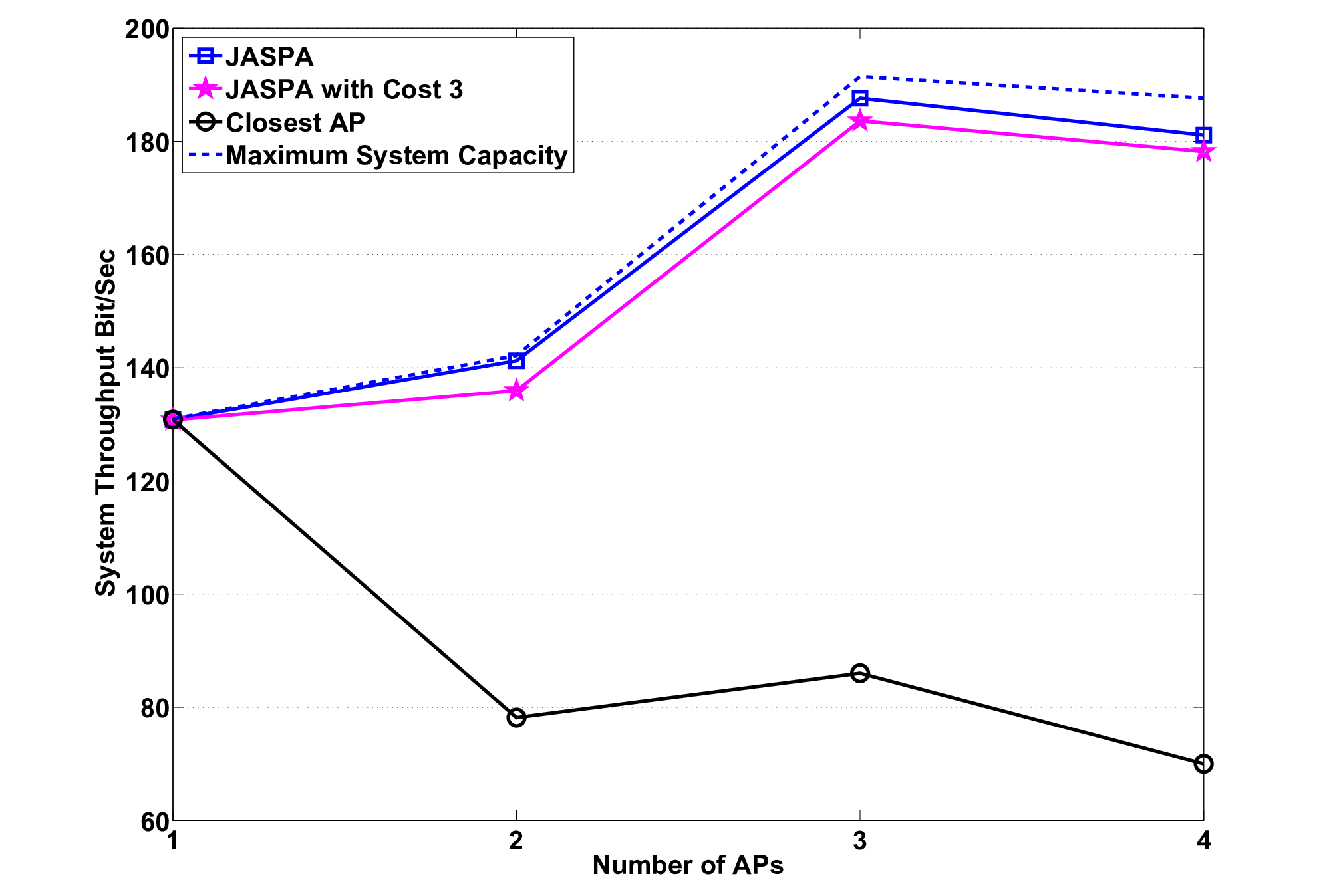
We first investigate a small networks with CUs, channels and APs, and compare the performance of JASPA related algorithms to the maximum network throughput that can be achieve for the same network. The maximum network throughput for a snapshot of the network is calculated by the following two steps: 1) for a specific AP-CU association profile, say , calculate the maximum network throughput (denoted by ) by summing up the maximum capacity44 4 For a single AP with fixed number of users and channel gains, the maximum capacity is the well-known multiple access channel sum capacity. of individual APs in the network; 2) enumerate all possible AP-CU association profiles, and find . We see the reason that we choose to focus on such relatively small networks in this experiment is that for a large network, the time it takes for the above exhaustive search procedure to find the maximum network throughput becomes prohibitive. The result is shown in Fig.5, where each point in the figure is obtained by averaging the results obtained by the algorithms on 100 independent snapshots of the network. We see that the JASPA algorithm performs very well with little throughput loss, while the closest AP algorithm, which separates the tasks of spectrum decision and spectrum sharing, performs poorly.
We then start to look at the performance of larger networks with 30 CUs, up to 16 APs and up to 128 channels. Fig. 6 shows the comparison of the performance of JASPA, JASPA with individual cost bit/sec and bit/sec, and the closest AP algorithm. We adopt the actual distance as the measure of “closeness” in the closest AP algorithm. Each point in this figure is the average of 100 independent runs of the algorithms.

in a 30 CU network.
Due to the prohibitive computation time required, we are unable to obtain the maximum system throughput for these relatively large networks. We instead compute the equilibrium system throughput that can be achieved in a non-cooperative game if all CUs are able to connect to multiple APs at the same time. We refer to this situation the K-connectivity network (the “K-Connectivity” network is similar in spirit to the “multi-homing” WLAN studied in [12]). It is clear that in the K-connectivity case, there is no need for the CUs to perform the AP selection algorithm, and the CUs in this network enjoy the flexibility of being able to connect to multiple APs at the same time. However, we observe that the performance of JASPA is very close to that of the “K-Connectivity” network.
From Fig. 6 we see that when the number of APs increases, the throughput of the JASPA algorithm becomes much better than the closest AP algorithm, a phenomenon that is partly due to the fact that for the closest AP algorithm, the separation of the AP selection and power allocation process results in the insufficient use of the spectrum: when the number of AP increases, it becomes increasingly more probable that several APs are idle because no CUs are close to them. Fig. 6, along with Fig. 4, also serve to confirm our early speculation that there indeed exists tradeoff of convergence speed and system throughput between JASPA and JASPA with connection cost.
VII Conclusion
In this paper, we addressed the joint AP association and power allocation problem in a CRN, and formulate it into a non-cooperative game with hybrid strategy space. We characterized the NE of this game, and provided distributed algorithms to reach such equilibrium. Empirical evidence gathered from simulation experiments suggests that the equilibrium has very promising quality in term of the system throughput.
The problem analyzed in this work, particularly the game with mixed strategy space, can be extended to solve many other problems, for example, the CRN with interference channel and segmented spectrum mentioned in section I-A. It will also be our future research topic to analyze the effect of random arrivals and departures of the CUs on the performance of the algorithm, and propose suitable heuristic dealing with these situations.
References
- [1] I. F. Akyildiz, W. Y. Lee, M. C. Vuran, and S. Mohanty, “A survey on spectrum management in cognitive radio networks,” IEEE Communications Magazine, pp. 40–48, April 2008.
- [2] L. Lai and H. E. Gamal, “The water-filling game in fading multiple-access channels,” IEEE Trans. on Inf. Theory, vol. 54, no. 5, 2008.
- [3] M. H. Islam, Y.-C. Liang, and A. T. Hoang, “Joint power control and beamforming for cognitive radio networks,” IEEE Transactions on Wireless Communications, vol. 7, no. 7, pp. 2415–2419, 2008.
- [4] S. V. Hanly, “An algorithm for combined cell-site selection and power control to maximize cellular spread spectrum capacity,” IEEE JSAC, vol. 13, no. 7, pp. 1332–1340, 1995.
- [5] R. D. Yates and C. Y. Huang, “Integrated power control and base station assignment,” IEEE Trans. on Veh. Tech., vol. 44, pp. 1427–1432, 1995.
- [6] T. Alpcan and T. Basar, “A hybrid noncooperative game model for wireless communications,” Annals of the International Society of Dynamic Games, vol. 9, pp. 411–429, 2007.
- [7] C. U. Sarayda, N. B. Mandayam, and D. J. Goodman, “Pricing and power control in a multicell wireless data network,” IEEE Journal on selected areas in communications, vol. 19, no. 10, pp. 1883–1892, 2001.
- [8] B. Kauffmann, F. Baccelli, and A. Chaintreau, “Measurement-based self organization of interfering 802.11 wireless access network,” in the Proceedings of IEEE INFOCOM, 2007, pp. 1451–1459.
- [9] Y. Bejerano, S. J. Han, and L. Li, “Fairness and load balancing in wireless LANs using association control,” IEEE/ACM Transactions on Networking, vol. 15, no. 3, pp. 560–573, 2007.
- [10] A. Kumar and V. Kumar, “Optimal association of stations and aps in an ieee 802.11 WLAN,” in the Proceedings of NCC, 2005.
- [11] A. Kumar, E. Altman, D. Miorandi, and M. Goyal, “New insights from a fixed-point analysis of single cell ieee 802.11 WLANs,” IEEE/ACM Trans. Netw., vol. 15, no. 3, pp. 588–601, 2007.
- [12] S. Shakkottai, E. Altman, and A. Kumar, “Multihoming of users to access points in WLANs: A population game perspective,” IEEE JSAC, pp. 1207–1215, 2007.
- [13] F. Wang, M. Krunz, and S. Cui, “Price-based spectrum management in CRN,” IEEE J. Sel. Topics Signal Process., vol. 2, no. 1, 2008.
- [14] Y. Wu and D. H. K. Tsang, “Distributed power allocation algorithm for spectrum sharing cognitive radio networks with qos guarantee,” in Proceedings of INFOCOM, 2009.
- [15] W. Yu, G. Ginis, and J. M. Cioffi, “Distributed multiuser power control for digital subscriber lines,” IEEE JSAC, vol. 20, pp. 1105–1115, 2002.
- [16] G. Scutari, D. P. Palomar, and S. Barbarossa, “Optimal linear precoding strategies for wideband noncooperative systems based on game theory – part I: Nash equilibria,” IEEE Trans. Sig. Process., vol. 56, no. 3, 2008.
- [17] L. Cao, L. Yang, and H. Zheng, “The impact of frequency-agility on dynamic spectrum sharing,” in IEEE DySPAN, April 2010.
- [18] Q. Zhao and B. M. Sadler, “A survey of dynamic spectrum access,” IEEE Signal Processing Magazine, no. 5, pp. 79–89, 2007.
- [19] M. Hong and A. Garcia, “Distributed uplink resource allocation in CRN:part I–II,” manuscript, http://people.virginia.edu/ ag7s/.