Quark-anti-quark potentials from Nambu-Bethe-Salpeter amplitudes on lattice
Abstract
Quark–anti-quark (-) potentials with finite quark masses are studied from the - Nambu-Bethe-Salpeter (NBS) wave functions in quenched lattice QCD. With the use of a method which has been recently developed in the derivation of nuclear forces from lattice QCD, we derive the - potentials from the NBS wave functions. We calculate the - NBS wave functions in pseudo-scalar and vector channels for several quark masses. The derived potentials at each quark mass in both channels show linear plus Coulomb form. We also discuss the quark-mass and channel dependence of the - potentials.
1 Introduction
An inter-quark potential is one of the most important ingredients of quantum chromodynamics (QCD). Experimentally, Regge slope [1] suggests that the inter-quark potentials show linear behavior at long distance. The string tension of the potentials between a quark and an anti-quark, , can be roughly estimated by hadron spectra using the relation with the spin and the mass of hadrons. At short distance, the inter-quark potential shows like the Coulomb interaction, which is, for example, suggested by the analogy between quarkonium and positronium. In fact, the linear plus Coulomb behaviors of the inter-quark potentials reproduce the low-lying hadron spectra well in quark models.
Theoretically, the study of the inter-quark potentials is challenging issue due to the non-perturbative nature of low energy phenomena in QCD. Lattice QCD simulation is the powerful tool for a numerical investigation in such a strong-coupling region of QCD. From the expectation value of Wilson loops, the potential for an infinitely heavy quark and anti-quark (- potential) and also the three-quark potential ( potential) can be obtained on lattices [2, 3]. The - potential from quenched lattice QCD simulations reveals the form of with and .
The actual inter-quark potentials suffer from the effect of quark motions, which is not included in the - potential. One can take into account the corrections coming from finite quark masses order by order with the use of the heavy quark effective field theory. The effective field theory utilizes the hierarchy of scales coming from the heavy quark mass and the relative velocity of heavy quarks, . The potential nonrelativistic QCD (pNRQCD) is such an effective field theory at the ultrasoft scale obtained by integrating out the hard scale and the soft scale [2, 4, 5, 6, 7]. It is convenient to employ pNRQCD to obtain the corrections of heavy quarkonium spectra to the heavy quark motion.
In this work, we study potentials between a quark and an anti-quark with a finite mass (- potentials) from quenched lattice QCD simulations. In order to explore the - potentials, we apply the systematic method which utilize the equal-time Nambu-Bethe-Salpeter (NBS) amplitudes to extract hadronic potentials [8, 9, 10, 11, 12, 13, 14, 15, 16, 17, 18, 19, 20] to the systems with a relatively light quark and an anti-quark. Due to the absence of the asymptotic fields of quarks, the reduction formula cannot be applied directly. Therefore, we assume that the equal-time NBS amplitudes for the - systems satisfy the Nambu-Bethe-Salpeter (NBS) equation with constant quark masses which could be considered as the constituent quark masses. By using the derivation of the relativistic three-dimensional formalism from the NBS equation developed by Lévy, Klein and Macke (LKM formalism) [22, 23, 24, 25], we shall obtain the - potentials without expansion in terms of . The preliminary results of the NBS wave functions and potentials of the - systems have been reported in Ref. [26].
The paper is organized as follows. In Sec. 2, we present our method to extract the - potentials. In Sec. 3, we show the lattice QCD setup. We then show our numerical results of the - wave functions and potentials in pseudo-scalar and vector channels for four different quark masses in Sec. 4. The obtained potentials reveal the linear plus Coulomb forms which are similar to the - potential from the Wilson loop. We perform fitting analyses of the - potential data. Sec. 5 is devoted to discussions and summary.
2 Method of the extraction of inter-quark potentials
Following the formulation to define the potentials on lattices [8, 9, 24], we show the basic equations to extract the - potentials on the lattice below. As shown in Ref. [24], the equal-time choice of the Nambu-Bethe-Salpeter (NBS) amplitudes satisfy the relativistic Schrödinger-type equation without an instantaneous approximation for original interaction kernels of the NBS equation. Therefore, we can start with the Schrödinger-type equation (which is reffered as LKM equation in Ref [24]) for the NBS wave function to define potentials:
| (1) |
where and denote the reduced mass of the - system and the non-relativistic energy, respectively, and we simply assume nonrelativistic kinematics. Note that the potential is generally energy-independent and non-local [9, 21]. In appendix A, we discuss potentials derived from the relativistic Schrödinger-type equation. The relativistic effects may be necessary to reproduce the meson mass spectra in the wide energy region.
For the two-nucleon case, it is proved that the Schrödinger-type equation is derived by using the reduction formula [9]. Due to the absence of asymptotic fields for confined quarks, we suppose that the - systems satisfy the NBS equation with their constant quark masses. In this study, constant quark masses are determined by half of vector meson masses , i.e., , as usually taken in constituent quark models. Then, one finds Schrödinger-type equation of Eq. (1) as a three-dimensional reduction of NBS equation by applying LKM [22, 23, 24, 25] method.
The energy-independent and non-local potential can be expanded in powers of the relative velocity of - systems at low energies,
| (2) | |||||
with
| (3) | |||||
| (4) |
where the term is of order , and , and being the tensor operator, orbital angular momentum and spin of the - systems, respectively. Note that the velocity expantion is different from the usual expansion, and the central force in the leading order includes not only linear and Coulomb terms but also higher order terms in the expansion such as the spin-spin interaction, , which is regarded as an order . This spin-spin interaction is an important ingredient of the mass formula in the constituent quark model. At the leading order, one finds
| (5) |
The effective leading order - potentials are studied in this work. The convergence of the expansion of can be checked by studying the energy dependence of the local potential as in Ref. [12]. When the local potential has little energy dependence, the potential between - is well described only by . In contrast, if the energy dependence is large, higher order terms are necessary. The study of the energy dependence of the local potential in the - systems is an important future work.
In order to obtain the NBS wave functions of the - systems on the lattice, let us consider the following equal-time NBS amplitudes
| (6) |
with the matrix elements
| (7) |
Here represents the Dirac -matrices, and stands for the source term which creates the - systems with spin-parity on the lattice. The NBS amplitudes in Eq. (6) are dominated by the lowest mass state of mesons with the mass at large time separation ():
| (8) | |||||
with being the volume of the box. Thus, the - NBS wave function is defined by the spatial correlation of the NBS amplitudes.
The NBS wave functions in S-wave states are obtained under the projection onto zero angular momentum (),
| (9) |
where represents 24 elements of the cubic rotational group, and the summation is taken for all these elements. Using Eq. (5) and Eq. (9), we will find the - potentials and NBS wave functions from lattice QCD.
3 Numerical setup of the lattice simulations
In this section, we show the actions and simulation parameters in this work. We employ the standard plaquette gauge action,
| (10) |
with . The plaquette is defined as
| (11) |
where is a link variable. As for quark fields , we adopt the standard Wilson fermion action,
| (12) | ||||
| (13) |
where is the hopping parameter.
We generate the quenched gauge fields on a lattice with QCD coupling , which corresponds to the physical volume and the lattice spacing fm [3, 27]. We measure the - NBS wave functions for four different hopping parameters , , , : the corresponding pseudo-scalar (PS) meson masses in the calculation are 0.94, 1.27, 1.77, 2.53GeV, and vector (V) meson masses =1.04, 1.35, 1.81, 2.55GeV, respectively. The number of configurations used in this simulation is 100 for each quark mass. The simulation parameters are summarized in Table 1. The calculation of the - NBS wave functions requires gauge fixing, because and operators are spatially separated at the sink time slice. Here we adopt Coulomb gauge, which is frequently used for studies of hadron spectroscopy in lattice QCD. As for the source operator of the - systems, we employ a static wall source in Eq. (6),
| (14) |
with the static wall quark operator
| (15) |
We note that gauge fixings and sink operators can be arbitrary chosen in the formalism, and all potentials with different gauge fixings and sink operators give the same physical observables, i.e., mass spectra and scattering lengths for instance. In this work, we employ Coulomb gauge and a local operator for sink operators. We can take another gauge fixing and sink operator, and the potential obtained with these conditions is generally different from that obtained in this work. In appendix B, we discuss the sink-operator dependence of the potential by using a gauge-invariant smeared operator for the sink.
4 Numerical results for the - potentials
First, we show the numerical results of the NBS wave functions in Fig. 1. Fig. 1(a) and (b) are the NBS wave functions for each quark mass in PS and V channels, respectively, at the time slice . The NBS wave functions mostly vanish at fm for all quark masses in both channels. This indicates that the spatial volume is large enough for the present calculations. The size of a wave function with a lighter quark mass becomes larger than that with a heavier one. Comparing the results in PS and V channels, little channel dependence between PS and V channels is found, although the quark-mass dependence of the wave functions is a bit larger for V channel.


In Fig. 2, we show the Laplacian parts of - potentials in Eq. (5), , for each quark mass and channel. Fig. 2(a) shows in PS channel for each quark mass at the time slice . As shown in Fig. 2, one can see that the potential form is similar to that obtained from Wilson loop, namely, the potential form looks like linear plus Coulomb form, although the derivation of the potentials is largely different between these two methods. Fig. 2(b) represents in V channel for each quark mass at the same time slice . The basic properties are similar to that in PS channel, although quark mass dependence is a bit larger for V channel.
Fig. 3(a) and (b) show the potentials with arbitrary energy shifts , i.e, in PS and V channels, respectively, for each quark mass at the time slice . Note that the quark mass is determined by the half of vector meson mass, , as mentioned in the previous section.
We perform fit analyses of the potentials in Fig. 3(a) and (b). For the fit function, we choose the linear plus Coulomb form, . We fit to the potential data for each quark mass and channel. We use the on-axis data with the range in the fit. The fit results are summarized in Table 2, and denoted by solid curves in Fig. 3(a) and (b). is around 0.5 for all the fit, which means the data are well described by the linear plus Coulomb form. We find moderate quark mass dependence of the string tension. The string tension becomes larger as increasing quark masses in both channels, and that for heaviest quark mass in our simulation is about 820MeV/fm, which is comparable to that obtained from an expectation value of the Wilson loop. On the other hand, the Coulomb coefficient strongly depends on quark masses. The Coulomb coefficient becomes small as increasing quark masses, and is roughly approaching to that obtained from an expectation value of the Wilson loop.
| Pseudo-scalar | Vector | ||||||
| MeV/fm | MeVfm | MeV/fm | MeVfm | ||||
| 0.32 | 0.63 | ||||||
| 0.35 | 0.61 | ||||||
| 0.46 | 0.44 | ||||||
| 0.31 | 0.23 | ||||||
Next, we perform another type of fit analyses. Assuming that the string tension is independent of the quark masses due to the quenched QCD simulations, where the contributions from quark loops are eliminated, we perform the fit by minimizing the general which is defined as with [30]. We call the fit “universal fit” here. The fit functions can be explicitly written by . The free parameters of the fit are for . In the fit, we choose the range of the potential data as . The fitting results are shown in Table 3. The general is achieved with for with MeV/fm. Since our simulation includes all the quark mass effects, is modified by the higher order effect of expansion.
| Pseudo-scalar | Vector | |
|---|---|---|
| MeVfm | MeVfm | |
We also perform another type of the universal fit with the fit function, , which contains correction terms, i.e., and . The term is predicted by pNRQCD and the effective string theory, respectively [28, 29]. In this fit, we use not only on-axis data but also off-axis data, and results are summarized in Table 4 (). As shown in Table 4, if we employ the fit function in which terms are taken into account, the Coulomb coefficients are smaller than those obtained and are comparable to the values from Wilson loop.
| Pseudo-scalar | Vector | |||||
| MeVfm | MeV | MeVfm2 | MeVfm | MeV | MeVfm2 | |
5 Discussion and summary
We have studied the inter-quark potentials between a quark and an anti-quark (- potentials) from the - Nambu-Bethe-Salpeter (NBS) wave functions. For this purpose, we have utilized the method which has been recently developed in the calculation of nuclear force from QCD [8, 9]. We have calculated the NBS wave functions for the - systems with four different quark masses in pseudo-scalar and vector channels and obtained the - potentials through the Schödinger-type equation. In this framework, the - potentials basically contains full quark motions with the finite masses. As a result, we have found that the shapes of the - potentials are the linear plus Coulomb form which is similar to the static - potential obtained from Wilson loop.
For the fitting, we have employed two types of fitting functions. One is the linear plus Coulomb form regarded as the leading order (LO) terms in the expansion. The other function includes the next leading order (NLO) terms in addition to LO terms. The fitting results with LO terms reveal that the Coulomb coefficients depend on the quark masses and are larger than those predicted from Wilson loop. On the other hand, if we have employed the NLO terms together with the LO terms, the Coulomb coefficients become smaller and are comparable to the value from Wilson loop. With the both fitting functions, we have obtained the string tension which is comparable to the value from Wilson loop.
This is the first step to study the - potentials from the NBS wave functions, and the main purpose of the present study is to show that the method is applicable to the - potentials. We find that the obtained - potential has the basic property of that obtained from Wilson loop. Therefore, this method can be used for the study of the - potentials with finite quark masses.
Acknowledgements.
The authors thank S. Aoki, T.Doi, T. Hatsuda, T. Inoue, N. Ishii, K. Murano, H. Nemura, K. Sasaki, T. Kawanai and S. Sasaki for the fruitful discussion. Y.I. also thanks N. Kaiser, A. Laschka and W. Weise for the useful discussion. The calculations were performed mainly by using the NEC-SX9 and SX8R at Osaka University, and partly by RIKEN Integrated Cluster of Clusters (RICC) facility. This project is supported in part by Grand-in-Aid for Japan Society for the Promotion of Science (No. 23-8687) and Scientific Research on Innovative Areas (No. 2004: 20105001, 20105003, 23105713).Appendix A Relativistic effect for the potential
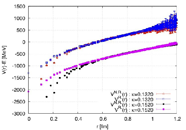
In the main part of the paper, we assume the non-relativistic kinematics for the Schrödinger-type equation. We here calculate the potential with relativistic kinematics to evaluate the relativistic effect for the - systems.
The relativistic Schrödinger-type equation for the - system in the continuum limit is written as
| (16) |
with the leading order potential of the velocity expansion. On a lattice, a discrete Fourier transformation of gives . Thus is replaced by , and the integral becomes a summation on lattice. Similar as the procedure in the main part, we obtain the potential from the discretized version of the relativistic Schrödinger-type equation of Eq. (16).
Fig. (4) is a comparison of potentials with relativistic kinematics, and non-relativistic potential shown in the main part. The relativistic potentials for () are shown by open square (filled square) in Fig. (4), while the non-relativistic potentials for () are shown by open circle (filled circle). As shown in Fig. (4), show the linear plus Coulomb behavior, and and is similar for large . On the other hand, for small , the difference between them becomes large as naturally expected, and the short distance differences of the potentials may contribute to reproducing higher energy states.
We calcurate the root mean square radius from the NBS wave function for the heaviest - system () employed in this work. Then we obtain fm, and the relativistic potential in Fig. (4) is consistent with non-relativistic one around 0.36 fm. Thus, for the heavy quark case such as the charm quark, we conclude that the non-relativistic potential picture gives the proper description of the heavy quarkonium. On the other hand, for the light quark such as strange quark, short range part of the relativistic potential differs from non-relativistic one. This shows that the relativistic effects starts to contribute to - systems.
Appendix B Potential from a gauge-invariant smeared operator
As we showed, the obtained potentials exhibit a Coulomb plus linear behavior. However, potentials with different operators are generally different. Therefore, the Cornell-like behavior is not universal. Here, we show a potential with a different operator from that used in the main part.
The NBS amplitude with gauge-invariant smeared sink operators is defined by
| (17) |
A schematic figure of the amplitude is shown in Fig. (5). The operator constructed by link variables connects and with a straight-line path. Here, the direction of is chosen to be the -, -, or -direction, i.e., on-axes.
Figure (6) shows a potential obtained from the smeared NBS amplitude, (red points for V channel and blue points for PS channel), and that obtained in Coulomb gauge, (green points for V channel and blue points for PS channel). Note that the data of are only calculated on the points with integral multiples of the lattice spacing , because in Eq. (17) is on-axis. shows the linear plus Coulomb behavior similar to that in Coulomb gauge, and, more over, the two potentials almost coincide. This fact shows that the gauge-invariant operator is also a suitable one for a constituent quark mass, and the Coulomb-gauge operator used in the main part is similar to the gauge-invariant operator of Eq. (17).


References
- (1) C. B. Chiu, Ann. Rev. Nucl. Part. Sci. 22, 255 (1972).
- (2) G. S. Bali, Phys. Rept. 343, 1 (2001).
- (3) T. T. Takahashi, H. Matsufuru, Y. Nemoto and H. Suganuma, Phys. Rev. Lett. 86, 18 (2001); T. T. Takahashi, H. Suganuma, Y. Nemoto and H. Matsufuru, Phys. Rev. D 65, 114509 (2002).
- (4) N. Brambilla, A. Pineda, J. Soto and A. Vairo, Nucl. Phys. B 566, 275 (2000); Rev. Mod. Phys. 77, 1423 (2005).
- (5) L. S. Brown and W. I. Weisberger, Phys. Rev. D 20, 3239 (1979).
- (6) E. Eichten and F. L. Feinberg, Phys. Rev. Lett. 43, 1205 (1979).
- (7) Y. Koma and M. Koma, Nucl. Phys. B769, 79 (2007).
- (8) N. Ishii, S. Aoki and T. Hatsuda, Phys. Rev. Lett. 99, 022001 (2007).
- (9) S. Aoki, T. Hatsuda and N. Ishii, Prog. Theor. Phys. 123, 89 (2010).
- (10) H. Nemura, N. Ishii, S. Aoki and T. Hatsuda, Phys. Lett. B673, 136 (2009).
- (11) H. Nemura et al. [HAL QCD and PACS-CS Collaboration], PoS LATTICE2009, 152 (2009).
- (12) K. Murano, N. Ishii, S. Aoki and T. Hatsuda, Prog. Theor. Phys. 125, 1225 (2011).
- (13) T. Inoue et al. [HAL QCD Collaboration], Prog. Theor. Phys. 124 , 591 (2010).
- (14) T. Inoue et al. [HAL QCD Collaboration], Phys. Rev. Lett. 106, 162002 (2011).
- (15) T. Doi et al. [HAL QCD Collaboration], arXiv:1106.2276 [hep-lat]; PoS LATTICE2010, 136 (2010).
- (16) K. Sasaki et al. [HAL QCD Collaboration], PoS LATTICE2010, 157(2010); arXiv:1012.5684 [nucl-th].
- (17) Y. Ikeda et al. [HAL QCD Collaboration], arXiv:1002.2309 [hep-lat]; Prog. Theor. Phys. Suppl. 186, 228 (2010).
- (18) T. Kawanai and S. Sasaki, Phys. Rev. D 82, 091501 (2010).
- (19) T. Hatsuda, arXiv:1101.1463 [nucl-th].
- (20) T. T. Takahashi and Y. Kanada-En’yo, Phys. Rev. D 82, 094506 (2010).
- (21) W. Królikowski and J. Rzewuski, Nuovo Cim. 4, 1212 (1956).
- (22) M. M. Levy, Phys. Rev. 88, 725 (1952).
- (23) A. Klein, Phys. Rev. 90, 1101 (1953).
- (24) A. Klein and T.-S. H. Lee, Phys. Rev. 10, 4308 (1974).
- (25) W. Macke, Phys. Rev. 91, 195 (1953).
- (26) Y. Ikeda and H. Iida, PoS LATTICE2010, 143 (2010).
- (27) T. Iritani, H. Suganuma and H. Iida, Phys. Rev. D 80, 114505 (2009).
- (28) M. Koma, Y. Koma and H. Wittig, PoS CONFINEMENT8, 105 (2008); Y. Koma and M. Koma, Prog. Theor. Phys. Suppl. No. 186, 205 (2010).
- (29) G. Perez-Nadal and J. Soto, Phys. Rev. D 79, 114002 (2009).
- (30) G. Hohler et al., Nucl. Phys. B 114, 505 (1976).