Distributed Uplink Resource Allocation in Cognitive Radio Networks – Part I: Equilibria and Algorithms for Power Allocation
Abstract
Spectrum management has been identified as a crucial step towards enabling the technology of a cognitive radio network (CRN). Most of the current works dealing with spectrum management in the CRN focus on a single task of the problem, e.g., spectrum sensing, spectrum decision, spectrum sharing or spectrum mobility. In this two-part paper, we argue that for certain network configurations, jointly performing several tasks of the spectrum management improves the spectrum efficiency. Specifically, our aim is to study the uplink resource management problem in a CRN where there exist multiple cognitive users (CUs) and access points (APs). The CUs, in order to maximize their uplink transmission rates, have to associate to a suitable AP (spectrum decision), and to share the channels used by this AP with other CUs (spectrum sharing). These tasks are clearly interdependent, and the problem of how they should be carried out efficiently and in a distributed manner is still open in the literature.
In this first part of the paper, we focus on the problem of spectrum sharing in a multi-channel CRN with a single AP. The insight gained from the analysis of this simpler network is used as the building block for analyzing the multiple AP network in the second part of this paper. We formulate the single AP spectrum sharing problem into a non-cooperative power allocation game, in which individual CUs aim at maximizing their transmission rate by finding the suitable power allocation on the available channels. Interestingly, we discover that the set of equilibrium solutions of this game possesses the following optimality properties: 1) any equilibrium solution is the optimum input power allocation scheme in the sense that it maximizes the sum rate of the network if joint decoding at the AP is employed; 2) asymptotically, when the number of channels becomes large, any equilibrium solution becomes a Frequency Division Multiple Access (FDMA) strategy, and the maximum system sum rate is achieved without joint decoding. We subsequently propose a set of algorithms for the CUs in the network to achieve such equilibrium solutions in distributed fashion.
I Introduction
I-A Motivation and Related Work
The problem of distributed spectrum management in the context of CRNs has been under intensive research recently. As pointed out by the authors of [2], spectrum management needs to address four main tasks: 1) spectrum sensing, techniques that ensure CUs to find the unused spectrum for communication; 2) spectrum decision, protocols that enable the CUs to decide on the best set of channels; 3) spectrum sharing, schemes that allow different CUs to share the same set of channels; 4) spectrum mobility, rules that require the CUs to leave the channel if licensed users are detected. Many efforts have been devoted to providing solutions to the individual tasks listed above. However, as we will see in this two-part paper, in some CRN scenarios, several of the above tasks become interdependent, and the CUs have to perform these tasks jointly to achieve best performance. We thus propose to provide solutions for the joint spectrum decision and spectrum sharing problems in a multi-channel multi-user CRN.
In this two-part paper we focus on investigating an important CRN configuration where such joint spectrum decision and spectrum sharing is desirable. Consider a network with multiple CUs and APs. The APs operate on non-overlapping spectrum bands, and the CUs need to connect to one of the APs for communication. At this stage the CUs essentially perform a spectrum decision task, in which they decide on the best spectrum band to use, i.e., the best AP to connect to. After the AP selection, the CUs can use multiple channels belonging to the associated AP concurrently for transmission, but different CUs interfere with each other if they use the same channel. At this stage the CUs perform a spectrum sharing task, in which multiple CUs use the same spectrum band for communication. This network is a generalization of the single AP network considered in previous literature, e.g., [3], [4] and [5]. It also bears sufficient similarity to the operational model of the IEEE 802.22 cognitive radio standard [6], in which multiple service providers install their respective APs to serve the same geographic region. In the considered network, the CUs face the spectrum decision problem when they select the AP, and they face the spectrum sharing problem when they try to dynamically allocate their communication power across the channels belonging to the selected AP. Clearly, these two problems are strongly interdependent, as on the one hand a particular CU has to select an AP before it can share the spectrum assigned to this AP with all the other CUs associated with it; on the other hand, after sharing the spectrum, an individual CU may have the incentive to switch to a different AP if it perceives that such action will increase its communication rate. A poor spectrum decision and spectrum sharing scheme will not only lead to unsatisfactory performance for individual CUs, but also result in an unstable system in which CUs are constantly unsatisfied with their current communication rates and consequently changing their AP associations and power allocation indefinitely.
In the first part of this paper, we focus on the spectrum sharing aspect of the above problem. Specifically, we study the uplink power allocation problem in a CRN with a single AP. This problem is important in its own right, and the insight gained from studying this problem serves in studying the more complicated network with multiple APs that we discuss in the second part of this paper.
Centralized strategies for resource allocation in multi-carrier single AP network has been extensively studied. In [7] and [8], a joint sub-carrier assignment and power allocation algorithm is proposed for downlink orthogonal frequency division multiplexing (OFDM) network with the objective to optimize utility functions related to throughput and fairness. It has been shown that when the utility function is properly chosen, the optimum access strategy is FDMA, and the downlink throughput can achieve Shannon capacity. In [9], the authors formulate the optimum (in the sense of minimizing the received mean square error) linear transceiver design problem in a multiple access (MAC) intersymbol interference (ISI) channel into an optimum uplink subcarrier allocation and power loading problem, and propose a strongly polynomial algorithm to determine such optimum strategy. [10] proposes a numerical method to compute the capacity of FDMA MAC channel as well as to (near-) optimally assign the channels. The proposed method assigns the channel to different users by solving a (convexly relaxed) optimization problem. [11] and [12] are two recent developments for uplink/downlink resource allocation in multi-carrier systems. The uplink optimality of OFDMA system has been discussed in [13], in which the authors derived sufficient conditions of the channel state as well as the received signal noise ratio for the OFDMA system to achieve maximum uplink system sum rate. We note that the centralized schemes usually assume that the AP carries out all the necessary computations and enforces the resultant optimum policies among the mobile users in the network.
However, such centralized scheme may not be applicable in networks where individual mobile users are autonomous or selfish and have the intention and the ability to deviate from the centralized policies (e.g., in the cognitive radio network). Consequently various distributed algorithms are proposed in the literature, for example, [14], [15] and [4]. In [14], a distributed power allocation scheme is proposed for uplink OFDM systems where the channel state is simplified to having only discrete levels. Notably, this scheme only requires that each user has the knowledge of its own channel state information (CSI), thus the signaling needed for the users to obtain the global CSI (as required by the algorithms proposed in, say, [3]) from the AP is greatly reduced. [15] is a recent work considering the uplink dynamic spectrum sharing problem in a multi-carrier multiple service provider cognitive network. The authors developed a distributed algorithm for the users to jointly choose the size of the spectrum as well as the amount of power for transmission. However, in this work the channel is considered to be flat for each user, as a result, the users only need to select the size of spectrum they need (because any portions of the spectrum of the same size is equivalent to the users), which greatly simplifies the analysis. In [4], the problem of distributed energy-efficient power control in uplink multi-carrier CDMA system is considered. The authors formulate the problem into a game-theoretic framework, and a distributed algorithm is proposed in which each user transmits only on its “best” channel. [16] considered a generalization of a multi-carrier MAC channel, and proposed a distributed iterative water-filling (IWF) algorithm to compute the maximum sum capacity of the system. It is worth mentioning that the algorithms proposed in [4] and [16] both require that the users update their transmission strategies sequentially, thus may result in slow convergence when the number of users in the system is large.
In this first part of the paper, we formulate the uplink spectrum sharing problem into a non-cooperative game, in which the CUs in the network try to maximize their individual transmission rate. Due to the structure of the considered multi-channel network, we are able to identify the proposed game as a potential game [17], in which the players in the game, although selfish by nature, behave as if they aim at jointly optimizing an objective function (which is called the potential function). Such underlying structure of the game allows us to characterize many optimality properties of the equilibrium solution. In particular, the maximum value of the potential function equals to the maximum sum rate achievable for the network. As a result, the CUs can be viewed as jointly optimizing the system sum rate. As far as we know, such interesting relationship between a spectrum sharing game and the system sum rate in multi-carrier single AP network has not been shown in the literature. We then propose three algorithms with convergence guarantees that allow the CUs to reach the equilibrium solution(s) in a distributed fashion. For the sake of rigor, we categorize our algorithms either as “weak convergent”, in which the individual CUs’ strategies converge to the set of equilibria, or as “strong convergent”, in which the individual CUs’ strategies converge to an equilibrium point. Such distinction is technical yet necessary, as we will point out in section IV-A, for the reason that unlike most other spectrum sharing games (e.g., [18], [19]), our game generally admits a connected set of equilibria, consequently it is possible, at least theoretically, for the algorithm to converge to the set of equilibria without converging to any equilibrium point.
I-B Organization of This Work and Notations
This part of the paper is organized as follows. In section II, we present the system under consideration, and formulate the spectrum sharing problem into a non-cooperative game. In section III, we give detailed analysis regarding to the property of the NE of the game. In section IV, we propose distributed algorithms and study their convergence properties. In section V, we show the numerical result. This part of the paper concludes in section VI.
Some notations used in this paper are specified as follows: we use bold lowercase and uppercase letters for vectors and matrices, respectively. The element of a matrix is denoted by . For a symmetric matrix , signifies that is positive semidefinite. The trace of a matrix is denoted by ; the determinant of a matrix is denoted by . is used to denote a identity matrix. For a vector , represents a diagonal matrix with its diagonal entries equal to the entries of the vector . We use to denote the spectral radius of the matrix .
II Problem Formulation
II-A System Model
We consider a wireless network with a set CUs and a single AP. Let us normalize the total available bandwidth to 1, and divide it equally into channels; let the set represents the set of available channels.
The followings
are our main assumptions of the network.
A-1) The available spectrum can be used exclusively by
the CRN, for a relative long period of time.
A-2) Each CU can concurrently use all the channels of the AP
for transmission, if desired.
A-3) The AP is equipped with single-user receivers.
Assumption A-1) can be achieved either under the spectrum property right model in which the licensed networks sell or lease the spectrum to the cognitive network for a period of time for exclusive use, or under the situation that the cognitive network exploits relatively static spectrum white spaces unused by local TV broadcast [20]. Assumption A-3) is congruent with the lack of coordination of the CUs, because an individual CU essentially treats other CUs’ transmission as noises. It also allows for implementation of low-complexity receivers at the AP. This assumption is generally accepted in designing distributed algorithm in multiple-access channels [3].
Let denote the complex Gaussian signal transmitted by CU on channel ; let denote the transmitted power of CU on channel . Let denote the white complex Gaussian environment noise experienced at the receiver of AP with mean zero and variance . Let denote the channel gain coefficient between CU and the AP on channel . The signal received at the AP on channel , denoted by , can then be expressed as:
| (1) |
Define ; ; . Then the received vector signal can then be expressed concisely as:
| (2) |
Let be CU ’s transmission power profile; let be the transmission profile of all other CUs except CU ; let be the system power profile. Define to be CU ’s maximum allowable transmission power, then its feasible space can be expressed as . In this network when single-user receiver is employed at the AP, and when assuming other CUs’ power profiles are fixed, the CU ’s maximum achievable rate can be expressed as [21]:
| (3) |
We assume that each CU has the knowledge of its own channel coefficients , and the quantity on every channel, which represents the sum of noise plus interference on each channel. This information can be obtained by the AP and fed back to each CU , as suggested in [4]. We do not assume that individual CU has any information regarding the other CUs’ channel coefficients; nor do we require that individual CU knows the power budget or the power allocations of other CUs.
The problem that the CUs are facing is that under the above sets of system constraints, how should they decide on the policy for efficiently sharing of the available spectrum in a distributed manner? In the following subsection, we formulate such spectrum sharing problem into a game-theoretical framework.
II-B A Non-Cooperative Game Formulation
In order to facilitate the development of a distributed algorithm, we model each CU as selfish agent, and its objective is to maximize its own transmission rate. More specifically, when is fixed, CU is interested in solving the following optimization problem:
| (4) |
The solution to this optimization problem is the well-known single-user water-filling solution [21]:
| (5) |
where is the dual variable for the sum-power constraints.
We introduce a non-cooperative spectrum sharing game where the players of the game are the CUs in the network, the utility of each player is its achievable transmission rate, and the strategy of each player is its transmit power profile. We denote this game as , where is the joint feasible region of all CUs.
The Nash Equilibrium (NE) of the above game is defined as the strategies satisfying [22]:
| (6) |
Intuitively, a NE of the game is a stable point of the system where no player has the incentive to deviate from its current strategy. In the following sections, we will first set out to analyze the properties of the set of NE of game , and then propose distributed algorithms to reach the set of NE.
III Characteristics and Optimality of the NE
III-A NE as Maximizers of the Potential Function
In order to facilitate the analysis, we introduce the notion of a potential function of the game . Define a concave function :
| (7) |
We can readily observe that the following identity is true for all and :
| (8) |
or similarly, for any and and for fixed ,
| (9) |
We call the function the potential function associated with the game . Due to the properties (8) and (9), we call the game a potential game. From [17], [23] and [24], we have the following theorem.
Theorem 1
A potential game, say , admits at least one pure-strategy NE. If the potential function associated with the potential game is concave, then a feasible strategy is a NE of the game if and only if it maximizes the potential function, i.e., .
In light of the above theorem, we immediately have the following Corollary.
Corollary 1
is a NE of the game if and only if
| (10) |
III-B NE as Optimum Input Strategies that Maximize the Network Sum Rate
It turns out that the potential function (7) has a nice physical interpretation. We show in this subsection that it can be related to the maximum sum rate achievable for the considered network. In order to make the above statement precise, we digress a little to consider the following sum capacity maximization problem of the vector MAC system.
Consider a vector MAC communication system [16] with users and a single AP. The users and the AP are both equipped with antennas. Assume the available bandwidth is . Let be user ’s transmitting vector signal; let be a matrix that represents the communication channel between user and the AP; let be the aggregated received signal at the AP; let be the additive Gaussian noise with covariance matrix . Then can be expressed as follows 11 1 Clearly the received signal has a similar form with that of the received signal in considered single AP network (cf. (2)), consequently, the results derived in this vector MAC system are instrumental in analyzing our single AP network. :
| (11) |
Let denote user ’s transmission/input covariance. The users are constrained in their individual power output, i.e., the input covariance of the users should satisfy . The capacity-achieving input distribution is known to be a complex Gaussian distribution, and the optimum set of input covariances that maximize the capacity of this system can be found by solving the following problem [16], [21]:
| (12) | ||||
where indicates the joint transmission covariance matrix. Notice, that the objective function is a concave function [21], hence, it admits a unique maximum value in the feasible region. However, this function is generally not strictly convex, and there are a (connected) set of optimum points that achieve such optimum value.
We have the following proposition regarding the input covariance matrices that maximizes the sum rate of the system.
Proposition 1
If is diagonal for each , and if is diagonal, then there must exist a set of diagonal input covariance matrices that is the optimum solution of the problem (12).
Proof:
We prove this proposition by contradiction. Consider the following convex problem:
| (13) | ||||
Suppose the set of diagonal matrices is an optimum solution of the problem (13), but it is not an optimum solution of the problem (12). For each user , let be the (unique) solution of the following optimization problem:
| (14) | ||||
Then from Theorem 1 of [16], and the assumption that is not optimum solution to the problem (12), there must be at least one user that, by changing its input covariance matrices from to , it can strictly improve the objective function, i.e., , such that .
Let us now find the optimum solution of the problem (14). Let , then is diagonal because , and are all diagonal. Clearly it is also semi-definite. Define a matrix with its elements satisfying:
Then solving problem (14) is equivalent to maximizing the function . From Hadamard’s inequality [21] and the fact that is diagonal, we have that:
where the equality is achieved if and only if is diagonal, and satisfying . Consequently, we conclude that the optimum covariance matrix of the problem (14) is a diagonal matrix. However, this contradicts the assumption that the set of covariance matrices is an optimum solution of the problem (13), because the new set of covariance matrices is a feasible solution to the problem (13), but . ∎
The proof of Proposition 1 points out that when and are diagonal, any solution to the optimization problem (13) must be an optimal solution to the original problem (12). In this case, the users only need to select the amount of power on each antenna (power loading transmission scheme) to achieve the maximum sum rate, and the objective function of (13) can be reduced to:
Clearly, when the channel matrices and the noise matrix are all diagonal, and the users choose the diagonal transmission strategy, the -user -antenna vector MAC channel introduced above is equivalent to the our previously considered -CU -channel single AP network (as can be seen from the equivalence of equation (2) and (11)), with the following correspondence of parameters: , and .
The vector MAC capacity maximization problems (12) or (13) can be readily seen as equivalent to the potential function maximization problem (10), and the maximum value of the potential function , say , corresponds to the maximum sum rate achievable for the considered N-CU, K-channel, single AP network. Corollary 1 implies that any NE of the game maximizes the potential function among the feasible solutions. Consequently it is also an optimal solution of (13), thus can be viewed as a set of optimal input covariance matrices (or optimum power loading scheme because of the diagnonality) that maximizes the achievable sum rate of the system.
However, this result does not imply that the sum of the CUs’ rate at a NE achieves the optimal system sum rate. We should point out here that in general, one needs to have both optimal transmission strategy and optimal receiving strategy to be able to achieve the MAC capacity. In our context, this is to say that in general, at a NE of the game , although the CUs’ transmission strategy is optimal, the sum of individual CUs’ rate should be less than the maximum achievable sum rate of the system (notice, that in our considered network, the assumption is that only single-user receiver is implemented at the AP, which is obviously not an optimal receiving strategy).
However, we observe that if a NE of the game represents a FDMA strategy, then the maximum system sum rate is achieved using only single-user receiver at the AP. More specifically, if a NE represents the FDMA strategy, then there is at most a single user transmitting on each channel (i.e., with ). Define the index set , we have that under a FDMA transmission strategy . Clearly in this case, the sum rate of the users (when the AP uses single-user receiver) achieves the maximum sum rate of the network:
| (17) |
where both and are from the FDMA property of the NE .
The question remains as in what situation does the NE of the game represents the FDMA transmission strategy. In the next subsection, we provide an answer to this question by looking at the situation when the available spectrum is arbirarily finely divided. i.e., .
III-C The Asymptotic Optimality of the NE
In this subsection, we consider the asymptotic situation in which the available bandwidth is arbitrarily finely divided. In this case, the transmission rate for each CU can be expressed as [21]:
| (18) |
where the channel gain can be viewed as the channel transfer function for CU to the AP; becomes the spectral density of the Gaussian noise experienced at the AP on channel ; denotes the transmit power spectral density of CU , i.e., indicates the amount of power CU transmits on frequency . In this case, the sum power constraint of each CU should be expressed as: , and the feasible region becomes: .
As before, a selfish CU is interested in solving the following optimization problem:
| (19) |
From the definition of the NE and the solution to the CU’s utility maximization problem (19), individual equilibrium transmit spectral must satisfy:
| (20) |
We have the following theorem characterizing the system equilibrium transmit spectral .
Theorem 2
When the available spectrum is arbitrarily finely divided, and the channel gains are generated according to some continuous distribution, then any NE of the game represents a FDMA transmission strategy (with probability 1). Moreover, any such NE is efficient, in the sense that the sum of individual users’ rates achieves the maximum system sum rate.
Proof:
We first show, by contradiction, that any NE represents the FDMA strategy.
Suppose for some channel realization , in the NE of the game a set of CUs are using the frequency . In another words, we assume the following:
| (21) |
Then the following is true for all :
| (22) |
Thus, for an arbitrary pair of CUs : . However, this equality is satisfied with probability zero (see the proof of Theorem 1 of [3]), because of the fact that and are constants, and that the channel coefficients are random variables drawn from continuous distributions (Rayleigh distribution or Rician distribution in fading channels). In summary, we claim that the equilibrium transmit power spectral follows a FDMA scheme with probability 1.
Due to the above FDMA frequency allocation scheme, when , it must be true that:
| (23) |
Consequently, we can have, for (thus ):
| (24) |
where is because of (23). From Theorem 2 of [25], we know that the -user FDMA scheme maximizes the system sum-rate for a Gaussian multiple access channel if the following is true:
| (25) | ||||
Comparing (23)–(24) with (25)–(III-C), we can readily identify that , and we conclude that achieves the maximum system sum rate. ∎
We see from the above derivation that the optimum channel assignment should take into consideration the following three factors [26]: 1) users’ channel quality; 2) users’ power budget; 3) the noise power. The results derived in Theorem 2 is desirable because in practical multi-carrier systems (e.g. OFDM system), the number of channels is indeed very large compared with the number of users in the system. Consequently, the NE of the spectrum sharing game represents a desirable outcome in which the CUs in the network share the spectrum efficiently. Interestingly, the authors of [3] has shown that the NE for a uplink power control game represents a time-sharing strategy (which can be viewed as dual to our FDMA strategy), but in a 2-user fading channel system which is very different from the system we consider.
Now the question becomes how such equilibrium point(s) can be reached by individual CU in a distributed fashion. In the next section, we provide three algorithms for such purpose.
IV The Proposed Algorithms and Convergence
From the argument in the previous section, we see that finding the NE of the game is equivalent to finding . This is a convex problem and can be solved in a centralized way if all the parameters of the system (e.g., , ) are known. However, in a distributed environment, where the CUs are selfish, uncoordinated and not well informed of other CUs’ channel coefficients and power budgets, it is not immediately clear how to find such NE point in a distributed fashion.
IV-A Inapplicability of Conventional IWF Algorithm
We first notice that our model of the network is a special case of a more general network with Gaussian interference channel that has been extensively studied recently, for example, in [18], [19], [27], [28]. In those works, the CUs are transmitter-receiver pairs, and they are interested in allocating their limited transmission power on the set of channels to maximize their individual transmission rate. We refer to this network as a Peer-to-Peer (PP) network, while referring to our network as a Access Point (AP) network. In the PP network, we use to denote the channel gain from CU ’s transmitter to CU ’s receiver on the channel; we use to denote the environmental noise power at the receiver of CU on channel . An individual CU , by transmiting on the channel, contributes to every other CU in the network the amount of interference at their respective receivers.
Now consider the scenario where all the CUs’ receivers are co-located. In this case, for a particular CU , the set of channel coefficients become equal to the value of ; the set of environment noises can be considered equal because the receivers are located at the same place. Consequently, the PP network is equivalent to the AP network.
At this point, we might come to the conclusion that the distributed algorithms developed for the PP network automatically works in the AP network, after all, the PP case is more general than the AP case. However, we show in the following that this is not true. As a matter of fact, the sufficient conditions for the convergence of most algorithms proposed for the PP network are not satisfied in the AP network. As an example, we consider the sufficient condition for the simultaneous IWF algorithm proposed in [27].
Define nonnegative matrices with their elements defined as follows:
Define another nonnegative matrix as follows:
From Theorem 1 in [27], we have that the simultaneous IWFA algorithm converges to the unique NE of the game if the following is true: . In the following, we prove that in AP scenario, this condition can not be satisfied.
From the Perron-Frobenius Theorem [29], we have that there must exist a vector , such that , where is the maximum norm of a matrix , and is defined as follows:
| (32) |
We next show that in the AP case, there could be no positive vector satisfying . Note that we have for all , componentwise, which implies ([29], Chapter 2, Proposition 6.2). Consequently, it is sufficient to prove that there exists , such that for all , we must have .
Choose any . Suppose there exists such that . This implies that: . Then it must be true that for every , , which is equivalent to say that the following inequalities are true simultaneously:
| (33) |
Recall that when reduced to AP configuration, we have that for all , . Using this equality and adding up inequalities in (33), we must have:
| (34) |
Because all the channel coefficients are greater than , the above inequality can not be satisfied for any . Consequently, we prove that there does not exist any such that . Thus, we must have that , which in turn says that for all , we must have , and this implies . We note further that since for any norm (Prop.A.20 in [29]), we must have that for arbitrary norm. Moreover, we can show similarly that for arbitrary norm, , and thus .
In order to further explain the reason why, in general, algorithms for the PP configuration fail to work in our AP configuration, we observe that almost all the algorithms designed for PP configuration rely on some restrictive conditions of the channel gains to ensure the uniqueness of the equilibrium. For example, in [18], the condition ensures the NE of the power allocation game is unique. However as we see in our previous argument, in the AP configuration such condition is not true for any realization of the channel gains. As a matter of fact, a straightforward consequence of Corollary 1 is that in general the AP configuration admits a (connected) set of equilibrium solutions, as the objective function of the optimization problem (10) is concave, but not strictly concave. A simple example illustrates this point.
Example 1
Consider the network with CUs, channels. Let , , , and let . We can show that both the following two system power profiles and are the NE for the game related to this network:
| (35) |
and
| (36) |
Clearly, from the concavity of the potential function, all the convex combinations of the solutions and also maximize the potential function, hence they are also NEs of the game .
We conclude the above argument by saying that although the AP network indeed is a special case of the more general PP network, for which distributed algorithms have been developed to reach the NE, these algorithms may not be directly applicable to the AP scenario. Indeed, we will see later in the simulation section, that by applying the simultaneous IWF algorithm directly to the AP network results in divergence.
IV-B Proposed Algorithm based on IWF: Weak Convergence
We now proceed to develop algorithms so that the CUs in the single AP network can distributedly reach the NE. In the following we propose two such algorithms.
Algorithm 1: Averaged Iterative-Water Filling Algorithm (A-IWF):
In each iteration , the CUs do the
following.
1) Calculate the best reply power allocation:
| (37) |
where ensures
,
and let
.
2) Adjust their power profiles simultaneously according to:
| (38) |
where the sequence satisfy and :
| (39) |
Algorithm 2: Sequential Iterative-Water Filling Algorithm (S-IWF):
In each iteration , the CUs adjust their power profiles
sequentially22
2
By “sequential” we mean that the CUs in the
set take turns in changing their power allocation, and
only a single CU gets to act at time . All other CUs keep their power allocation as in time .
according to:
| (40) |
The convergence properties of the above two algorithms are stated in the following two propositions.
Proposition 2
If all the CUs in the network employ A-IWF algorithm, then their individual power profiles converge to the set of NE of game .
Proof:
Define . Define . Then from the system point of view the A-IWF algorithm can be written concisely as:
| (41) |
We first introduce two lemmas. The proof of Lemma 1 can be found in Appendix A, and we omit the proof of Lemma 2 for brevity.
Lemma 1
There must exist a constant , with , such that .
Lemma 2
For two arbitrary vectors and , and for arbitrary norm , there must exist two constants , and such that
| (42) |
In order to conform to the convention in convex optimization, we define the function , and we see that is convex.
Then from the well known Descent Lemma (Lemma 2.1 in [29]), and Lemma 2 we have that:
| (43) | ||||
| (44) |
Because goes to , then when large enough, , and is monotonically decreasing. Combined with the fact that is lower bounded, then is a convergent sequence.
From (43), we have that
It is clear that is upper bounded, and we have , so . Because converges, we must have
| (45) |
From Lemma 1, we have
Consequently it is clear that we must have . We show in the following that in fact we have a stronger result that . Suppose not, then . In this case there must exist a such that the subsequences and are both infinite.
For a specific , the following is true:
| (46) |
Thus, there exists a such that for all , we must have .
We also have the following:
| (47) |
which implies
| (48) |
From our previous derivation, we also have Then for any there must exists a such that for all :
Take , and take , then we have
| (49) |
which implies . This is a contradiction to (48). Thus, we conclude that , and consequently .
From we see that the limit point of any converging subsequence of , say , must satisfy , which is sufficient condition to ensure that is a NE of the game . Consequently must maximize the function (from Corollary 1), and this implies that the entire sequence converges to the value . It also implies that the sequence converge the set of NE of the game , or in other words, every limit point of is a NE of the game . ∎
Proposition 3
If all the CUs in the network employ S-IWF algorithm, then their individual power profiles converge to the set of NE of game . Moreover, the potential function is non-decreasing with respect to iteration step , i.e., .
Proof:
It is easy to see that this algorithm corresponds to the nonlinear Gauss-Seidel algorithm in solving constrained optimization problem [29], thus the general theory for the convergence of algorithm can be applied (e.g., [29] Proposition 3.9). ∎
The S-IWF algorithm is actually a simplification of the algorithm proposed in [16]. We introduce this algorithm here and briefly discuss its convergence analysis because it will be useful in our analysis in the second part of this paper. We need to point out here that the convergence behaviors characterized for A-IWF and S-IWF are set convergence, i.e., the distance between the sequence and the set of NE decreases to zero. Theoretically, it is possible that multiple limit points exist for such sequence, hence this convergence behavior is weaker than the “strong convergence”, in which the sequence admits a single limit point in the set of NE. In practice though, convergence of the sequence is always observed 33 3 The S-IWF algorithm proposed in [16] for vector MAC channel also converges to the set of optimum points similarly as ours, and in practice it has been observed that such algorithm always converges to a single point.. However, for the sake of rigor, in the next subsection we propose a third algorithm which converges strongly to the set of NE.
IV-C Proposed Algorithm based on Gradient Descent: Strong Convergence
Algorithm 3: Projected Gradient Descent Algorithm:
In each iteration , the CUs do the
following.
1) Calculate the gradient of the potential function:
| (50) |
2) Adjust their power profiles simultaneously according to:
| (51) |
where the sequence satisfy and (39); the operator represents the projection on to the space .
Clearly, this algorithm is based on the classical projected gradient descent algorithm for solving nonlinear optimization problem, but with diminishing stepsize . In order to prove the convergence of this algorithm, we first introduce the notion of Quasi-Fejér convergence [30], [31], [32].
Definition 1
A sequence is Quasi-Fejér convergent to a set if for every there is a sequence such that and
Theorem 3
If is Quasi-Fejér convergent to a nonempty set , then is bounded. If furthermore a limit point of belongs to , then , i.e., the sequence converges to a single point in .
Using the notion of Quasi-Fejér convergence, we have the following strong convergence result for Algorithm 3. Please see Appendix B for proof.
Proposition 4
The projected gradient descent algorithm is Quasi-Fejér convergent to the set of NE of game , with error term . Moreover, the sequence generated by this algorithm converges to a point in the set of NE.
IV-D Discussion
We first note that all the three algorithms proposed in the previous subsections can be carried out in a distributed fashion. That is, in order to carry out the computations in each iteration (mainly to compute or ) of the algorithms, the CUs do not need to know the behavior of other CUs in the network. Instead, an individual CUs only needs to know the aggregated interference plus noise (IPN) contributed by all other CUs on each channel: . As suggested by [4], this information can be fed back to the CUs by the AP. In fact, the AP only needs to broadcast the quantity to the CUs, and individual CU can subtract its contribution and calculate . We can also show that, similarly as in the previous two subsections, that a more general case of the algorithm where each CU adopts different sequences of update coefficients (say ) also converges, as long as each sequence satisfies the conditions in (39).
As stated previously, the theoretical categorization of the algorithms by their convergence behaviors is necessary, because it is generally not possible for the game to have a single equilibrium point. Although for the algorithms in both categories, the potential function (or equivalently the sum capacity) converges to the single optimum point, the convergence behavior of the underlying CUs’ strategies are more involved. Simply claiming the algorithm to be ‘‘convergent” might be too ambiguous and sometimes misleading 44 4 Indeed, in many situations convergence to a set leads to oscillation of the sequence. For example, the sequence converges to the set {-1, 0, 1}. . We observe that many iterative water-filling based algorithms for calculation of the capacity for vector MAC and broadcast channels, for example the algorithms in [13], [16] and [33], can only be theoretically proven to be weakly convergent (in which the optimum capacity is attained in the limit, but the underlying sequence converges to the optimum set), although in practice they generally converges to a single optimum point.
For the descent algorithm, note that if the update step size is a constant, then the algorithm is also weakly convergent (see Prop. 3.4 of [29])55 5 Consequently, most algorithms proposed for potential games based on projected gradient methods (e.g., those in [24]) can also be categorized as weak convergence when the potential function is concave but not strictly concave.. The descent algorithm with diminishing step size is also used in [34] for network utility maximization with feedback uncertainty, and the problem considered is very different from ours. We remark that, strong convergence does not imply fast convergence. Indeed, although we are able to show that the projected gradient decent algorithm converges strongly (which is theoretically appealing), in practice it tends to converge much slower than A-IWF and S-IWF. As such, in the second part of this paper, we will only choose A-IWF and S-IWF as building blocks for the joint AP selection and power allocation algorithm.
V Simulation Results
In this section, we demonstrate the performance of the proposed algorithm. We have the following general settings for the simulation. We place multiple CUs and the AP randomly in a area; we let denote the distance between CU and AP , then the channel gains between CU and AP . Unless otherwise noted, are independently drawn from an exponential distribution with mean (i.e., is assumed to have Rayleigh distribution).
Fig. 1 shows a typical realization of the three algorithms analyzed in this paper, in a network with CUs and channels. It is seen that the values of the potential function generated by these algorithms converge to the maximum system capacity quickly, but the sum rate of the CUs (hence individual power profiles) converges slowly for the projected gradient descent algorithm.

Fig. 3 partly quantifies the convergence speed of different algorithms. In this figure, we compare the absolute difference between the maximum system sum rate and the values of the potential function generated by different algorithms (i.e., ), in a network with user and channels. We observe that both the A-IWF and S-IWF algorithms converge relatively fast while the projected gradient descent algorithm, as seen in Fig.1, converges slowly. We have also studied the performance of simultaneous IWF algorithm [27], which clearly diverges in our single AP network. Such phenomenon has been partially explained in Section IV-A. In Fig. 3, we characterize the convergence behavior of the sum of the CUs’ rate , by plotting the relative difference between and : . Such metric can be viewed as related to the convergence speed of the algorithm. We see that for network with 128 channels and with increasing number of CUs, S-IWF converges increasingly slowly. Such behavior of the S-IWF is intuitively considering the sequential nature of the algorithm. We note that each point in both of these two figures is an average of 100 independent runs of the respective algorithms.


In Section III-C, we have predicted that for a fixed number of CUs, when the number of channels becomes large, the CUs tend to share the spectrum in a FDMA fashion, and the sum rate of the users approaches the maximum achievable system sum rate. Fig. 5 and Fig. 5 justify these claims. We say that a channel is collided if more than one CUs are using this channel. We say that a (event of) collision occurs if two CUs are using the same channel66 6 If CUs are using the same channel, then there are a total number of collisions occurred.. In Fig. 5, we plot the relationship between the number of channels in the system and the number of collided channels as well as the total number of collisions. Clearly, as the number of channels becomes large, both of the above quantities decreases. We also observe that when the number of channels becomes large, the number of collided channels tends to be the same as the total number of collisions, a phenomenon which implies that there tend to be no more than two CUs using a collided channel. In Fig. 5, we show the relative difference between the sum rate of the CUs after iteration of the A-IWF algorithm and the maximum sum rate (i.e., ), when the number of channels becomes large. The decreasing of such relative difference is an indication of increased efficiency of the spectrum sharing among the CUs. We note that each point in both of these two figures is again an average of 100 independent runs of the respective algorithms.

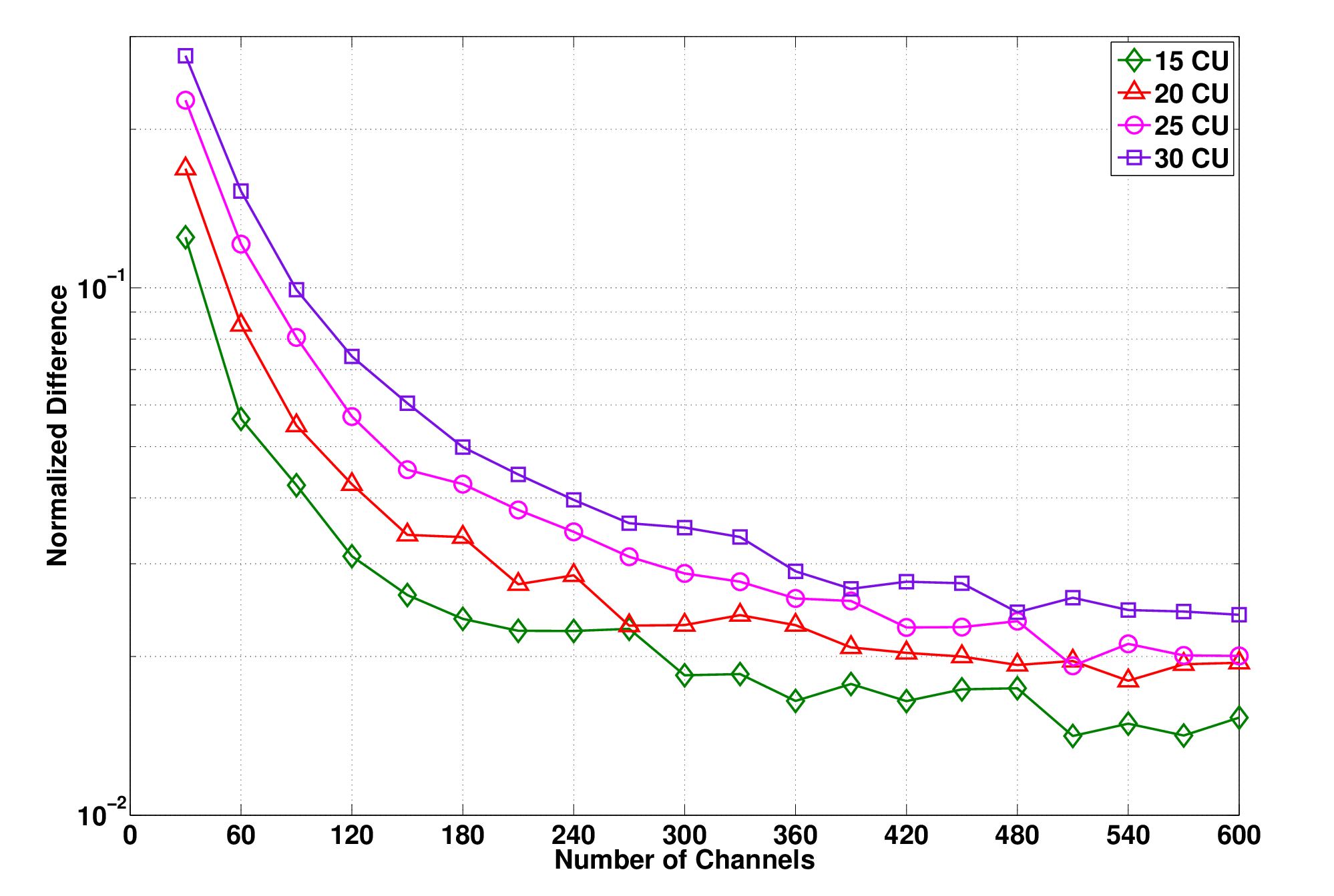
To quantify the overall efficiency of the spectrum sharing scheme, we plot the normalized system sum rate in Fig. 7 for the network with different number of CUs and different number of channels. Clearly the sharing scheme becomes more efficient when the number of channels becomes large. Notice, that in all the previous simulation experiments, we assume that the channel coefficients of a particular CU to be independent. This is true when the width of each channel is comparable to the coherent bandwidth, denoted as [35]. However, when we divide a fixed spectrum band with arbitrarily large number of channels, the coherent bandwidth eventually becomes larger than the channel width. Indeed, as mentioned in [13], in practice the parallel frequency selective channels are usually correlated. As a result, in Fig .7 we study the spectrum sharing efficiency for a network with CUs and with networks of different channel coherent bandwidth (recall that our total available bandwidth is normalized to ). For reference we also plot the case where the channels are assumed to be independent. We observe that large coherent bandwidth reduces the sharing efficiency. This phenomenon can be explained by noticing that when the channel becomes correlated, the event of collision is more likely to happen, as shown in Table I. We again note that each point in both of these two figures and each entry in the table is an average of 100 independent runs of the respective algorithms.


| Independent | |||||
|---|---|---|---|---|---|
| Total Collision, K=300 | 6.40 | 7.91 | 11.12 | 11.60 | 14.69 |
| Total Collided Channels, K=300 | 6.13 | 7.70 | 10.06 | 10.63 | 13.90 |
| Total Collision, K=600 | 4.31 | 5.21 | 6.00 | 7.65 | 12.67 |
| Total Collided Channels, K=600 | 4.30 | 5.07 | 5.81 | 7.61 | 12.19 |
VI Conclusion
In this first part of the paper, we formulate the uplink spectrum sharing problem in a single AP CRN into a non-cooperative game framework. We identify that this game belongs to the family of games called the “potential games”, and we characterize the properties of the proposed game. We then propose three algorithms with different convergence properties that allows the CUs in the network to access the spectrum in a distributed fashion. From simulation we see that the proposed algorithms are able to reach the equilibria of the spectrum sharing game, which represent a set of efficient spectrum sharing strategies.
In the next part of the paper, we will study jointly the spectrum sharing and spectrum decision problem in a CRN with multiple APs. We will see how the algorithms developed in this part of the paper can be used for constructing efficient and distributed joint spectrum decision and spectrum sharing strategies.
Appendix A Proof of Lemma 1
Proof:
We first prove Lemma 1. We need to show that the following is true:
| (52) |
where . It is sufficient to show that for all , there must exist a constant such that: In the following, we will set out to prove that for all , there must exist a with , such that:
| (53) |
We notice that
| (54) | ||||
| (55) |
We also observe the following equality:
| (56) |
This can be readily concluded from our previous observation that from each user’s point of view, it is beneficial to allocate all its power for communication. Using (56), we see that in order to prove (53), it is sufficient to prove that for all and such that
| (57) |
there exists such that:
| (58) | ||||
| (59) |
If the above is true, we can take , then for all that satisfies (57), we have
| (60) |
Consequently, (53) can be established.
Let us look at the term first. Let us simplify the notation by denoting , where . Because , we must have that , consequently, we have:
| (61) |
We then look at the term . We can, similarly as above, also simplify it as . Because , we must have that , consequently, we have:
| (62) |
As a result of (61) and (62), in order to prove (58), it is sufficient to prove that there exists such that:
| (63) |
We see that (63) is equivalent to
| (64) |
Define , and similarly, we have that the above inequality can be simplified to:
| (65) |
Now notice that:
| (66) |
and we have from (61) and (62) that
| (67) |
We have that . Consequently, (65) is equivalent to
| (68) |
Now it is clear that we can always find such a , that satisfies the above inequality, because the fact that is always bounded above and strictly greater than 0 (, ).
Appendix B Proof of Proposition 4
Proof:
The projected gradient algorithm can be written as: , where . We first show that at least one limit point of the sequence is a NE of the game . From the Projection Theorem ([29] Sec 3.3 Prop. 3.2) we have that:
| (69) |
Consequently, we have:
| (70) |
Similarly as in (43), we invoke the descent lemma:
| (71) |
where is from (70); is because of the non-expansiveness of the projection operator:
| (72) |
Thus there must exist a time such that , . From the fact that the function is lower bounded, we must have that the sequence converges. An immediate consequence of this result (cf. equation (45)) is that:
| (73) |
Let be a limit point of the sequence , then we must have that . This fact combined with the projection theorem implies that for any , the following is true:
| (74) |
The last inequality shows that , and consequently, is a NE of the game .
We then show that the sequence is Quasi-Fejér convergent to the set of NE. Using again the Projection Theorem, and (with a little abuse of notation) take to be any NE solution, we have:
| (75) |
This is equivalent to:
| (76) |
where is because of the fact that is concave: . The distance between and a arbitrary vector can be expressed as follows:
| (77) |
where is from (76) and the definition of that . Now let us take Then we have:. From (70) and (73) we conclude is non-negative and summable sequence. Because is an arbitrary NE point, from Definition 1 the sequence is Quasi-Fejér convergent to the set of NE of game . The first part of this proof show that a limit point of belongs to the set of NE, consequently, by applying Theorem 3, we see that converges to a point in the set of NE. ∎
References
- [1] M. Hong, A. Garcia, and J. Barrera, “Joint distributed AP selection and power allocation in cognitive radio networks ” in the Proceedings of the IEEE INFOCOM, 2011, accepted.
- [2] I. F. Akyildiz, W. Y. Lee, M. C. Vuran, and S. Mohanty, “A survey on spectrum management in cognitive radio networks,” IEEE Communications Magazine, pp. 40–48, April 2008.
- [3] L. Lai and H. E. Gamal, “The water-filling game in fading multiple-access channels,” IEEE Transactions on Information Theory, vol. 54, no. 5, 2008.
- [4] F. Meshkati, M. Chiang, H. V. Poor, and S. C. Schwartz, “A game-theoretic approach to energy-efficient power control in multicarrier CDMA systems,” IEEE Journal on Selected Areas in Communications, vol. 24, pp. 1115–1129, 2006.
- [5] M. H. Islam, Y.-C. Liang, and A. T. Hoang, “Joint power control and beamforming for cognitive radio networks,” IEEE Transactions on Wireless Communications, vol. 7, no. 7, pp. 2415–2419, 2008.
- [6] C. R. Stevenson, G. Chouinard, Z. Lei, W. Hu, S. J. Shellhammer, and W. Caldwell, “IEEE 802.22: the first cognitive radio wireless regional area network standard,” Comm. Mag., vol. 47, no. 1, pp. 130–138, 2009.
- [7] G. Song and Y. Li, “Cross-layer optimization for OFDM wireless networks–part I: Theoretical framework,” IEEE Transactions on Wireless Communications, vol. 4, no. 2, pp. 614–624, 2005.
- [8] G. Song and Y. Li, “Cross-layer optimization for OFDM wireless networks–part II: Algorithm development,” IEEE Transactions on Wireless Communications, vol. 4, no. 2, pp. 625–634, 2005.
- [9] Z-.Q. Luo, T. N. Davidson, G. B. Giannakis, and K. M. Wong, “Transceiver optimization for block-based multiple access through ISI channels,” IEEE Transactions on Signal Processing, vol. 52, no. 4, pp. 1037–1052, 2004.
- [10] W. Yu and J. M. Cioffi, “FDMA capacity of gaussian multiple-access channel with isi,” IEEE Transactions on Communications, vol. 50, no. 1, pp. 102–111, 2002.
- [11] K. Kim, Y. Han, and S.-L Kim, “Joint subcarrier and power allocation in uplink OFDMA systems,” IEEE Communication Letters, vol. 9, pp. 526–528, 2005.
- [12] T. Liu, C. Yang, and L.-L. Yang, “A lower-complexity subcarrier-power allocation scheme for frequency-division multiple-access scheme,” IEEE Transactions on Wireless Communications, vol. 11, no. 5, pp. 1571–1576, 2010.
- [13] H. Li and H. Liu, “An analysis of uplink OFDM optimality,” IEEE Transactions on Wireless Communications, vol. 6, no. 8, pp. 2972–2983, 2007.
- [14] G. He, S. Gault, M. Debbah, and E. Altman, “Distributed power allocation game for uplink ofdm systems,” in Proc. WiOPT, 2008, pp. 515–521.
- [15] J. Acharya and R. D. Yates, “Dynamic spectrum allocation for uplink users with heterogeneous utilities,” IEEE Transactions on Wireless Communications, vol. 8, no. 3, pp. 1405–1413, 2009.
- [16] W. Yu, W. Rhee, S. Boyd, and J. M. Cioffi, “Iterative water-filling for gaussian vector multiple-access channels,” IEEE Transactions on Information Theory, vol. 50, no. 1, pp. 145–152, 2004.
- [17] D. Monderer and L. S. Shapley, “Potential games,” Games and Economics Behaviour, vol. 14, pp. 124–143, 1996.
- [18] G. Scutari, D. P. Palomar, and S. Barbarossa, “Optimal linear precoding strategies for wideband noncooperative systems based on game theory – part I: Nash equilibria,” IEEE Transactions on Signal Processing, vol. 56, no. 3, 2008.
- [19] Z-. Q. Luo and J-.S. Pang, “Analysis of iterative waterfilling algorithm for multiuser power contorl in digital subscriber lines,” EURASIP Journal on Applied Signal Processing, vol. 2006, pp. 1–10, 2006.
- [20] Q. Zhao and B. M. Sadler, “A survey of dynamic spectrum access,” IEEE Signal Processing Magazine, , no. 5, pp. 79–89, 2007.
- [21] T. M. Cover and J. A. Thomas, Elements of Information Theory, second edition, Wiley, 2005.
- [22] M. J. Osborne and A. Rubinstein, A Course in Game Theory, MIT Press, 1994.
- [23] R. Deb, “A characterization of differentiable potential games,” http://www.econ.yale.edu/ rd287/.
- [24] G. Scutari, S. Barbarossa, and D. P. Palomar, “Potential games: A framework for vector power control problems with coupled constraints,” in the Proceedings of ICASSP 06, 2006.
- [25] R. Cheng and S. Verdu, “Gaussian multiaccess channels with isi: Capacity region and multiuser water-filling,” IEEE Transactions on Information Theory, vol. 39, no. 3, pp. 773–785, 1993.
- [26] W. Yu, G. Ginis, and J. M. Cioffi, “Distributed multiuser power control for digital subscriber lines,” IEEE Journal on Selected Areas in Communications, vol. 20, no. 5, pp. 1105–1115, 2002.
- [27] G. Scutari, D. P. Palomar, and S. Barbarossa, “Optimal linear precoding strategies for wideband noncooperative systems based on game theory – part II: Algorithms,” IEEE Transactions on Signal Processing, vol. 56, no. 3, 2008.
- [28] K. W. Shum, K. K. Leung, and C. W. Sung, “Convergence of iterative waterfilling algorithm for gaussian interference channels,” IEEE Journal on Selected Area in Communications, vol. 25, pp. 1091–1100, 2007.
- [29] D. P. Bertsekas and J. N. Tsitsiklis, Parallel and Distributed Computation: Numerical Methods, 2nd ed, Athena Scientific, Belmont, MA, 1997.
- [30] Y. M. Ermoliev, “On the method of generalized stochastic gradient and quasi-fejér sequences,” Cybernetics, 1969.
- [31] A. N. Iusem, B. F. Svaiter, and M. Teboulle, “Entropy-like proximal methods in convex programming,” Mathematics of Operations Research, 1994.
- [32] R. Burachik, L. M. G. Drummond, and A. N. Iusem, “Full convergence of the steepest descent method with inexact line search,” Optimization, pp. 137–146, 1995.
- [33] N. Jindal, W. Rhee, S. Vishwanath, S. A. Jafar, and A. Goldsmith, “Sum power iterative water-filling for multi-antenna gaussian broadcast channels,” IEEE Transactions on information theory, vol. 51, no. 4, 2005.
- [34] J. Zhang, D. Zhang, and M. Chiang, “The impact of stochastic noisy feedback on distributed network utility maximization,” IEEE Transactions on Information Theory, , no. 2, pp. 645–665, 2008.
- [35] A. Goldsmith, Wireless Communications, Combridge University Press, New York, 2005.