跳到论文正文
W Papers独立论文阅读器 arXiv:1102.1871 论文正文 计算阅读时间 · 0%
引用这篇论文根据当前论文元数据生成,正式投稿前建议核对。


License: arXiv.org perpetual non-exclusive license
arXiv:1102.1871v1 [math.PR] 09 Feb 2011

Multivariate piecewise linear interpolation of a random field

Konrad Abramowicz Affiliation: Department of Mathematics and Mathematical Statistics    Oleg Seleznjev Affiliation: Umeå University, SE-901 87 Umeå, Sweden
August 24, 2026
Abstract

We consider a multivariate piecewise linear interpolation of a continuous random field on a dd-dimensional cube. The approximation performance is measured by the integrated mean square error. Multivariate piecewise linear interpolator is defined by NN field observations on a locations grid (or design). We investigate the class of locally stationary random fields whose local behavior is like a fractional Brownian field in mean square sense and find the asymptotic approximation accuracy for a sequence of designs for large NN. Moreover, for certain classes of continuous and continuously differentiable fields we provide the upper bound for the approximation accuracy in the uniform mean square norm.

Keywords: approximation, random field, sampling design, multivariate piecewise linear interpolator

1 Introduction

Let a random field X⁡(𝐭),𝐭∈[0,1]dX(\mathbf{t}),\,\mathbf{t}\in[0,1]^{d}, with finite second moment be observed at finite number of points. Suppose further that the points are vertices of hyperrectangles generated by a grid in a unit hypercube. At any unsampled point we approximate the value of the field by a piecewise linear multivariate interpolator, which is a natural extension of a conventional one-dimensional piecewise linear interpolator. The approximation accuracy is measured by the integrated mean squared error. This paper aims modelling random fields with given accuracy based on a finite number of observations. Following Berman (1974), we extend the concept of local stationarity for random fields and focus on fields satisfying this condition. For quadratic mean (q.m.) continuous locally stationary random fields, we derive the exact asymptotic behavior of the approximation error. A method is proposed for determining the asymptotically optimal knot (sample points) distribution between the mesh dimensions. We also study optimality of knot allocation along coordinates of the sampling grid. Additionally, for q.m. continuous and continuously differentiable fields satisfying Hölder type conditions, we determine asymptotical upper bounds for the approximation accuracy.

The problem of random field approximation arises in many research and applied areas, like Gaussian random fields modelling (Adler and Taylor, 2007; Brouste et al., 2007), environmental and geosciences (Christakos, 1992; Stein, 1999), sensor networks (Zhang and Wicker, 2005), and image processing (Pratt, 2007). The upper bound for the approximation error for isotropic random fields satisfying Hölder type conditions is given in Ritter et al. (1995). Müller-Gronbach (1998) consider affine linear approximation methods and hyperbolic cross designs for fields with covariance function of tensor type. An optimal allocation of the observations for Gaussian random fields with product type kernel is investigated in Müller-Gronbach and Schwabe (1996). Su (1997) studies limit behavior of the piecewise constant estimator for random fields with a particular form of covariance function. Benhenni (2001) investigates exact asymptotics of stationary spatial process approximation based on an equidistant sampling. The approximation complexity and the curse of dimensionality for additive random fields are broadly discussed in Lifshits and Zani (2008). In one-dimensional case, the piecewise linear interpolation of continuous stochastic processes is considered in, e.g., Seleznjev (1996). Results for approximation of locally stationary processes can be found in, e.g., Seleznjev (2000); Hüsler et al. (2003); Abramowicz and Seleznjev (2011). Ritter (2000) contains a very detailed survey of various random process and field approximation problems. For an extensive studies of approximation problems in deterministic setting, we refer to, e.g., Nikolskii (1975); de Boor et al. (2008); Kuo et al. (2009).

The paper is organized as follows. First we introduce a basic notation. In Section 2, we consider a piecewise multivariate linear approximation of continuous fields which local behavior is like a fractional Brownian field in mean square sense. We derive exact asymptotics and a formula for the optimal interdimensional knot distribution. In the second part of this section, we provide an asymptotical upper bound for the approximation accuracy for q.m. continuous and differentiable fields satisfying Hölder type conditions. In Section 3, we present the results of numerical experiments, while Section 4 contains the proofs of the statements from Section 2.

1.1 Basic notation

Let X=X⁡(𝐭),t∈𝒟:=[0,1]dX=X(\mathbf{t}),\textbf{t}\in{\cal D}:=[0,1]^{d}, be a random field defined on a probability space (Ω,ℱ,P)(\Omega,\mathscr{F},P). Assume that for every t, the random variable X⁡(t)X(\textbf{t}) lies in the normed linear space L2​(Ω)=L2​(Ω,ℱ,P)L^{2}(\Omega)=L^{2}(\Omega,\mathscr{F},P) of random variables with finite second moment and identified equivalent elements with respect to PP. We set ‖ξ‖:=(E​ξ2)1/2||\xi||:=\left(\mathrm{E}\xi^{2}\right)^{1/2} for all ξ∈L2​(Ω)\xi\in L^{2}(\Omega) and consider the approximation based on the normed linear spaces of q.m. continuous and continuously differentiable random fields denoted by 𝒞⁡(𝒟){\cal C}({\cal D}) and 𝒞1​(𝒟){\cal C}^{1}({\cal D}), respectively. We define the norm for any X∈𝒞⁡(𝒟)X\in{\cal C}({\cal D}) by setting

||X||p:=(∫𝒟‖X⁡(t)‖p​𝑑t)1/p,1≤p<∞,\left|\left|\,X\,\right|\right|_{p}:=\left(\int_{\cal D}||X(\textbf{t})||^{p}d\textbf{t}\right)^{1/p},\qquad 1\leq p<\infty,

and ||X||∞:=max𝐭∈𝒟⁡||X⁡(𝐭)||\left|\left|\,X\,\right|\right|_{\infty}:=\max_{\mathbf{t}\in{\cal D}}\left|\left|\,X(\mathbf{t})\,\right|\right|. For p=2p=2, we call the norm integrated mean squared norm and the corresponding measure of approximation accuracy the integrated mean squared error (IMSE).

Now we introduce the classes of random fields used throughout this paper. For k≤dk\leq d, let 𝐥=(l1,…,lk)\mathbf{l}=(l_{1},\ldots,l_{k}) be a vector of positive integers such that ∑j=1klj=d\sum_{j=1}^{k}l_{j}=d, and let Li:=∑j=1ilj,i=0,…kL_{i}:=\sum_{j=1}^{i}l_{j},i=0,\ldots k, L0=0L_{0}=0, be the sequence of its cumulative sums. Then the vector 𝐥\mathbf{l} defines the l-decomposition of 𝒟{\cal D} into 𝒟1×𝒟2×…​𝒟k{\cal D}^{1}\times{\cal D}^{2}\times\ldots{\cal D}^{k}, with the ljl_{j}-cube 𝒟j=[0,1]lj{\cal D}^{j}=[0,1]^{l_{j}}, j=1,…,kj=1,\ldots,k. For any 𝐬∈𝒟\mathbf{s}\in{\cal D}, we denote the coordinates vector corresponding to the jj-th component of the decomposition by 𝐬j\mathbf{s}^{j}, i.e.,

𝐬j=𝐬j(𝐥):=(sLj−1+1,…,sLj)∈𝒟j,j=1,…,k.\mathbf{s}^{j}=\mathbf{s}^{j}(\mathbf{l}):=(s_{L_{j-1}+1},\ldots,s_{L_{j}})\in{\cal D}^{j},\quad j=1,\ldots,k.

For a vector 𝜶=(α1,…,αk)\boldsymbol{\alpha}=(\alpha_{1},\ldots,\alpha_{k}), 0<αj<20<\alpha_{j}<2, j=1,…,kj=1,\ldots,k, and the decomposition vector 𝐥=(l1,…,lk)\mathbf{l}=(l_{1},\ldots,l_{k}), we define

||𝐬||𝜶:=∑j=1k||𝐬j||αj for all ​𝐬∈𝒟\left|\left|\,\mathbf{s}\,\right|\right|_{\boldsymbol{\alpha}}:=\sum_{j=1}^{k}\left|\left|\,\mathbf{s}^{j}\,\right|\right|^{\alpha_{j}}\quad\mbox{ for all }\mathbf{s}\in{\cal D}

with the Euclidean norms ‖𝐬j‖,j=1,…,k||\mathbf{s}^{j}||,j=1,\ldots,k.

For a random field X∈𝒞⁡([0,1]d)X\in{\cal C}([0,1]^{d}), we say that
(i) X∈𝒞𝐥𝜶​([0,1]d,C)X\in{\cal C}_{\mathbf{l}}^{\boldsymbol{\alpha}}([0,1]^{d},C) if for some 𝜶\boldsymbol{\alpha}, 𝐥\mathbf{l}, and a positive constant CC, the random field XX satisfies the Hölder condition, i.e.,

||X⁡(𝐭+𝐬)−X⁡(𝐭)||2≤C​||𝐬||𝜶 for all ​𝐭,𝐭+𝐬∈[0,1]d,\left|\left|\,X(\mathbf{t+s})-X(\mathbf{t})\,\right|\right|^{2}\leq C\left|\left|\,\mathbf{s}\,\right|\right|_{\boldsymbol{\alpha}}\qquad\mbox{ for all }\mathbf{t},\mathbf{t+s}\in[0,1]^{d}, (1)

(ii) X∈ℬ𝐥𝜶​([0,1]d,c⁡(⋅))X\in{\cal B}_{\mathbf{l}}^{\boldsymbol{\alpha}}([0,1]^{d},c(\cdot)) if for some 𝜶\boldsymbol{\alpha}, 𝐥\mathbf{l}, and a vector function c⁡(𝐭)=(c1​(𝐭),…,ck​(𝐭))c(\mathbf{t})=(c_{1}(\mathbf{t}),\ldots,c_{k}(\mathbf{t})), 𝐭∈[0,1]d\mathbf{t}\in[0,1]^{d}, the random field XX is locally stationary, i.e.,

||X⁡(𝐭+𝐬)−X⁡(𝐭)||2∑j=1kck​(𝐭)​||𝐬j||αj→1as ​𝐬→0​ uniformly in ​𝐭∈[0,1]d,\frac{\left|\left|\,X(\mathbf{t+s})-X(\mathbf{t})\,\right|\right|^{2}}{\sum_{j=1}^{k}c_{k}(\mathbf{t})\left|\left|\,\mathbf{s}^{j}\,\right|\right|^{\alpha_{j}}}\rightarrow 1\quad\mbox{as }\mathbf{s}\rightarrow 0\mbox{ uniformly in }\mathbf{t}\in[0,1]^{d}, (2)

with positive and continuous functions c1​(⋅),…,ck​(⋅)c_{1}(\cdot),\ldots,c_{k}(\cdot). We assume additionally that for j=1,…,kj=1,\ldots,k, the function cj​(⋅)c_{j}(\cdot) is invariant with respect to coordinates permutation within the jj-th component.

For the classes 𝒞𝐥𝜶{\cal C}_{\mathbf{l}}^{\boldsymbol{\alpha}} and ℬ𝐥𝜶{\cal B}_{\mathbf{l}}^{\boldsymbol{\alpha}}, the withincomponent smoothness is defined by the vector 𝜶=(α1,…,αk)\boldsymbol{\alpha}=(\alpha_{1},\ldots,\alpha_{k}). We denote the vector describing the smoothness for each coordinate by 𝜶∗=(α1∗,…,αd∗)\boldsymbol{\alpha}^{*}=(\alpha_{1}^{*},\ldots,\alpha_{d}^{*}), where αi∗=αj\alpha_{i}^{*}=\alpha_{j}, i=Lj−1+1,…,Lji=L_{j-1}+1,\ldots,L_{j}, j=1,…,kj=1,\ldots,k.

Example 1. Let 𝐦=(m1,…,mk)\mathbf{m}=(m_{1},\ldots,m_{k}) be a decomposition vector of [0,1]m[0,1]^{m}, and m=∑j=1kmjm=\sum_{j=1}^{k}m_{j}. Denote by B𝜷,𝐦​(𝐭)B_{\boldsymbol{\beta},\mathbf{m}}(\mathbf{t}), 𝐭∈[0,1]m\mathbf{t}\in[0,1]^{m}, 𝜷=(β1,…,βk)\boldsymbol{\beta}=(\beta_{1},\ldots,\beta_{k}), 0<βj<20<\beta_{j}<2, j=1,…,kj=1,\ldots,k, an mm-dimensional fractional Brownian field with covariance function r⁡(𝐭,𝐬)=12​(‖𝐭‖𝜷+‖𝐬‖𝜷−||𝐭−𝐬||𝜷)r(\mathbf{t},\mathbf{s})=\frac{1}{2}\left(||\mathbf{t}||_{\boldsymbol{\beta}}+||\mathbf{s}||_{\boldsymbol{\beta}}-||\mathbf{t}-\mathbf{s}||_{\boldsymbol{\beta}}\right). Then B𝜷,𝐦B_{\boldsymbol{\beta},\mathbf{m}} has stationary increments,

‖B𝜷,𝐦​(𝐭+𝐬)−B𝜷,𝐦​(𝐭)‖2=‖𝐬‖𝜷,𝐭,𝐭+𝐬∈[0,1]m,||B_{\boldsymbol{\beta},\mathbf{m}}(\mathbf{t+s})-B_{\boldsymbol{\beta},\mathbf{m}}(\mathbf{t})||^{2}=||\mathbf{s}||_{\boldsymbol{\beta}},\quad\mathbf{t},\mathbf{t+s}\in[0,1]^{m},

and therefore, B𝜷,𝐦∈ℬ𝐦𝜷​(𝒟,c⁡(⋅))B_{\boldsymbol{\beta},\mathbf{m}}\in{\cal B}_{\mathbf{m}}^{\boldsymbol{\beta}}({\cal D},c(\cdot)) with local stationarity functions c1​(𝐭)=…=ck​(𝐭)=1c_{1}(\mathbf{t})=\ldots=c_{k}(\mathbf{t})=1, 𝐭∈[0,1]m\mathbf{t}\in[0,1]^{m}. In particular, if k=1k=1, then Bβ,m​(𝐭),𝐭∈[0,1]mB_{\beta,m}(\mathbf{t}),\,\mathbf{t}\in[0,1]^{m}, 0<β<20<\beta<2, m∈ℕm\in\mathbbm{N}, is an mm-dimensional fractal Brownian field with covariance function

r⁡(𝐭,𝐬)=12​(‖𝐭‖β+‖𝐬‖β−‖𝐭−𝐬‖β),𝐭,𝐭+𝐬∈[0,1]m.r(\mathbf{t},\mathbf{s})=\frac{1}{2}\left(||\mathbf{t}||^{\beta}+||\mathbf{s}||^{\beta}-||\mathbf{t}-\mathbf{s}||^{\beta}\right),\quad\mathbf{t},\mathbf{t+s}\in[0,1]^{m}. (3)

For X∈𝒞1​([0,1]d)X\in{\cal C}^{1}([0,1]^{d}), we write Xj′​(𝐭),𝐭∈[0,1]dX_{j}^{\prime}(\mathbf{t}),\,\mathbf{t}\in[0,1]^{d}, to denote a q.m. partial derivative of XX with respect to the jj-th coordinate, and say that X∈𝒞1,𝜶∗​([0,1]d,C)X\in{\cal C}^{1,\boldsymbol{\alpha}^{*}}([0,1]^{d},{C}) if there exist a vector 𝜶∗=(α1∗,…,αd∗)\boldsymbol{\alpha}^{*}=(\alpha_{1}^{*},\ldots,\alpha_{d}^{*}) and a positive constant CC such that each partial derivative Xj′X_{j}^{\prime} is Hölder continuous with respect to the jj-th coordinate, i.e., if for all 𝐭,𝐭+𝐬∈[0,1]d\mathbf{t},\mathbf{t+s}\in[0,1]^{d},

‖Xj′​(t1,…,tj+sj,…,td)−Xj′​(t1,…,tj,…,td)‖2≤C​|sj|αj∗j=1,…,d.||X^{\prime}_{j}(t_{1},\ldots,t_{j}\!+\!s_{j},\ldots,t_{d})-X^{\prime}_{j}(t_{1},\ldots,t_{j},\ldots,t_{d})||^{2}\leq C|s_{j}|^{\alpha_{j}^{*}}\quad j=1,\ldots,d. (4)

Moreover, we say that X∈𝒞𝐥1,𝜶​([0,1]d,C)X\in{\cal C}_{\mathbf{l}}^{1,\boldsymbol{\alpha}}([0,1]^{d},{C}) with 𝜶=(α1,…,αk)\boldsymbol{\alpha}=(\alpha_{1},\ldots,\alpha_{k}) if X∈𝒞1,𝜶∗​([0,1]d,C)X\in{\cal C}^{1,\boldsymbol{\alpha}^{*}}([0,1]^{d},{C}) and for a given partition vector 𝐥\mathbf{l}, αi:=αLi−1+1∗=…=αLi∗\alpha_{i}:=\alpha_{L_{i-1}+1}^{*}=\ldots=\alpha_{L_{i}}^{*}, i=1,…,ki=1,\ldots,k.

Let XX be sampled at NN distinct design points TNT_{N}. We consider cross regular sequences of sampling designs TN:={𝐭𝐢=(t1,i1,…,td,id):𝐢=(i1,…,id)T_{N}:=\{\mathbf{t}_{\mathbf{i}}=(t_{1,i_{1}},\ldots,t_{d,i_{d}}):\mathbf{i}=(i_{1},\ldots,i_{d}), 0≤ik≤nk∗0\leq i_{k}\leq n_{k}^{*}, k=1,…,d}k=1,\ldots,d\} defined by the one-dimensional grids

∫0tj,ihj∗(v)dv=inj∗,i=0,1,…,nj∗,j=1,…,d,\int_{0}^{t_{j,i}}h_{j}^{*}(v)dv=\frac{i}{n_{j}^{*}},\quad i=0,1,\ldots,n_{j}^{*},\quad j=1,\ldots,d,

where hj∗​(s)h^{*}_{j}(s), s∈[0,1]s\in[0,1], j=1,…,dj=1,\ldots,d, are positive and continuous density functions, say, withindimensional densities, and let

h∗​(𝐭):=(h1∗​(t1),…,hd∗​(td)).{h}^{*}(\mathbf{t}):=(h_{1}^{*}(t_{1}),\ldots,h_{d}^{*}(t_{d})).

The interdimensional knot distribution is determined by a vector function π:ℕ→ℕd\pi:\mathbbm{N}\to\mathbbm{N}^{d}:

π∗​(N):=(n1∗​(N),…,nd∗​(N)),\pi^{*}(N):=(n_{1}^{*}(N),\ldots,n_{d}^{*}(N)),

where limN→∞nj∗​(N)=∞\lim_{N\to\infty}n_{j}^{*}(N)=\infty, j=1,…,dj=1,\ldots,d, and the condition

∏j=1d(nj∗​(N)+1)=N\prod_{j=1}^{d}(n_{j}^{*}(N)+1)=N

is satisfied. We suppress the argument NN for the sampling grid sizes nj∗=nj∗​(N)n_{j}^{*}=n_{j}^{*}(N), j=1,…,dj=1,\ldots,d, when doing so causes no confusion. Cross regular sequences are one of the possible extensions of the well known regular sequences introduced by Sacks and Ylvisaker (1966). The introduced classes of random fields have the same smoothness and local behavior for each coordinate of components generated by a decomposition vector 𝐥\mathbf{l}. Therefore in the following, we use only approximation designs with the same within- and interdimensional knot distributions within the components. Formally, for the partition generated by a vector 𝐥=(l1,…,lk)\mathbf{l}=(l_{1},\ldots,l_{k}), we consider cross regular designs TNT_{N}, defined by the functions h:=(h1,…,hk)h:=(h_{1},\ldots,h_{k}) and π⁡(N):=(n1​(N),…,nk​(N))\pi(N):=(n_{1}(N),\ldots,n_{k}(N)), as follows:

hi∗(⋅)≡hj(⋅),ni∗=nj,i=Lj−1+1,…,Lj,j=1,…,k.h_{i}^{*}(\cdot)\equiv h_{j}(\cdot),\quad n_{i}^{*}=n_{j},\quad i=L_{j-1}+1,\ldots,L_{j},\quad j=1,\ldots,k.

We call the functions h1​(⋅),…,hk​(⋅)h_{1}(\cdot),\ldots,h_{k}(\cdot) and π⁡(N)\pi(N) withincomponent densities and intercomponent knot distribution, respectively. The corresponding property of a design TNT_{N} is denoted by: TNT_{N} is c​R​S​(h,π,𝐥)cRS(h,\pi,\mathbf{l}).

For a given cross regular sampling design, the hypercube 𝒟{\cal D} is partitioned into M=∏j=1dnj∗M=\prod_{j=1}^{d}n_{j}^{*} disjoint hyperrectangles 𝒟𝐢{\cal D}_{\mathbf{i}}, 𝐢=(i1,…,id)\mathbf{i}=(i_{1},\ldots,i_{d}), 0≤ik≤nk∗−10\leq i_{k}\leq n_{k}^{*}-1, k=1,…,dk=1,\ldots,d. Let 𝟏d=(1,…,1)\mathbf{1}_{d}=(1,\ldots,1) denote a dd-dimensional vector of ones. The hyperrectangle 𝒟𝐢{\cal D}_{\mathbf{i}} is determined by the vertex 𝐭𝐢=(t1,i1,…,tj,id)\mathbf{t_{i}}=(t_{1,i_{1}},\ldots,t_{j,i_{d}}) and the main diagonal 𝐫𝐢=𝐭𝐢+𝟏d−𝐭𝐢\mathbf{r}_{\mathbf{i}}=\mathbf{t}_{\mathbf{i}+\mathbf{1}_{d}}-\mathbf{t_{i}}, i.e.,

𝒟𝐢:={𝐭:𝐭=𝐭𝐢+𝐫𝐢∗𝐬,𝐬∈[0,1]d},{\cal D}_{\mathbf{i}}:=\left\{\mathbf{t}:\mathbf{t}=\mathbf{t}_{\mathbf{i}}+\mathbf{r}_{\mathbf{i}}*\mathbf{s},\mathbf{s}\in[0,1]^{d}\right\},

where ′∗′{}^{\prime}*^{\prime} denotes the coordinatewise multiplication, i.e., for 𝐱=(x1,…,xd)\mathbf{x}=(x_{1},\ldots,x_{d}) and 𝐲=(y1,…,yd)\mathbf{y}=(y_{1},\ldots,y_{d}), 𝐱∗𝐲:=(x1​y1,…,xd​yd)\mathbf{x}\ast\mathbf{y}:=(x_{1}y_{1},\ldots,x_{d}y_{d}).

For a random field X∈𝒞⁡(𝒟)X\in{{\cal C}}({\cal D}), define a multivariate piecewise linear interpolator (MPLI) with knots TNT_{N}

XN​(𝐭):=XN​(X,TN)​(𝐭)=E𝜼​X​(𝐭𝐢+𝐫𝐢∗𝜼),𝐭∈𝒟𝐢,𝐭=𝐭𝐢+𝐫𝐢∗𝐬,X_{N}(\mathbf{t}):=X_{N}(X,T_{N})(\mathbf{t})=\mathrm{E}_{\boldsymbol{\eta}}X(\mathbf{t_{i}}+\mathbf{r_{i}}*\boldsymbol{{\eta}}),\quad\mathbf{t}\in{\cal D}_{\mathbf{i}},\,\,\mathbf{t}=\mathbf{t_{i}}+\mathbf{r_{i}}*\mathbf{s},

where 𝜼=(η1,…,ηd){\boldsymbol{\eta}}=(\eta_{1},\ldots,\eta_{d}) and η1,…,ηd\eta_{1},\ldots,\eta_{d} are auxiliary independent Bernoulli random variables with means s1,…,sds_{1},\ldots,s_{d}, respectively, i.e., ηj∈B​e​(sj)\eta_{j}\in{Be}(s_{j}), j=1,…,dj=1,\ldots,d. Such defined interpolator is continuous and piecewise linear along all coordinates.

Example 2. Let d=2d=2, N=4N=4, 𝒟=[0,1]2{\cal D}=[0,1]^{2}. Then 𝐭=𝐬\mathbf{t}=\mathbf{s}, 𝐫=(1,1)\mathbf{r}=(1,1),

XN​(𝐭)=E𝜼​X​(𝜼)=X⁡(0,0)​(1−t1)​(1−t2)+X⁡(1,0)​t1​(1−t2)+X⁡(0,1)​(1−t1)​t2+X⁡(1,1)​t1​t2,\displaystyle X_{N}(\mathbf{t})=\mathrm{E}_{\boldsymbol{\eta}}X(\boldsymbol{\eta})=X(0,0)(1-t_{1})(1-t_{2})+X(1,0)t_{1}(1-t_{2})+X(0,1)(1-t_{1})t_{2}+X(1,1)t_{1}t_{2},

and XNX_{N} is a conventional bilinear interpolator (Lancaster and Šalkauskas, 1986, see, e.g.,).

We introduce some additional notation used throughout the paper. For sequences of real numbers unu_{n} and vnv_{n}, we write un≲vnu_{n}\lesssim v_{n} if limn→∞un/vn≤1\lim_{n\to\infty}u_{n}/v_{n}\leq 1 and un≍vnu_{n}\asymp v_{n} if there exist positive constants c1,c2c_{1},c_{2} such that c1​un≤vn≤c2​unc_{1}u_{n}\leq v_{n}\leq c_{2}u_{n} for nn large enough.

2 Results

Let Bβ,m​(𝐭),𝐭∈ℝ+mB_{\beta,m}(\mathbf{t}),\mathbf{t}\in\mathbb{R}^{m}_{+}, 0<β<20<\beta<2, m∈ℕm\in\mathbb{N}, denote an mm-dimensional fractional Brownian field with covariance function (3). For any 𝐮∈ℝ+m\mathbf{u}\in\mathbb{R}^{m}_{+}, we denote

bβ,m​(𝐮):=∫[0,1]m||Bβ,m​(𝐮∗𝐬)−E𝜼​Bβ,m​(𝐮∗𝜼)||2​𝑑𝐬,b_{\beta,m}(\mathbf{u}):=\int_{[0,1]^{m}}\left|\left|\,B_{\beta,m}(\mathbf{u}\ast\mathbf{s})-\mathrm{E}_{\boldsymbol{\eta}}B_{\beta,m}(\mathbf{u}\ast\boldsymbol{\eta})\,\right|\right|^{2}d\mathbf{s},

where 𝜼=(η1,…,ηm)\boldsymbol{\eta}=(\eta_{1},\ldots,\eta_{m}), and η1,…,ηm\eta_{1},\ldots,\eta_{m} are independent Bernoulli random variables ηj∈Be(sj),j=1,…,m\eta_{j}\in Be(s_{j}),\,j=1,\ldots,m. Then bβ,m​(𝐮)b_{\beta,m}(\mathbf{u}) is the squared IMSE of approximation for Bβ,m​(𝐮∗𝐭),𝐭∈[0,1]mB_{\beta,m}(\mathbf{u}\ast\mathbf{t}),\mathbf{t}\in[0,1]^{m}, by the MPLI with 2m2^{m} observations in the vertices of unit hypercube.

In the following theorem, we provide an exact asymptotics for the IMSE of a local stationary field approximation by MPLI when a cross regular sequence of sampling designs is used.

Theorem 1

Let X∈ℬ𝐥𝛂​(𝒟,c⁡(⋅))X\in{\cal B}_{\mathbf{l}}^{\boldsymbol{\alpha}}({\cal D},c(\cdot)) be a random field approximated by the MPLI XN​(X,TN)X_{N}(X,T_{N}), where TNT_{N} is c​R​S​(h,π,𝐥)cRS(h,\pi,\mathbf{l}). Then

||X−XN||22∼∑j=1kvjnjαj>0​ as ​N→∞,\left|\left|\,X-X_{N}\,\right|\right|_{2}^{2}\sim\sum_{j=1}^{k}\frac{v_{j}}{n_{j}^{\alpha_{j}}}>0\mbox{ as }N\to\infty,

where

vj=∫𝒟cj​(𝐭)​bαj,lj​(Hj​(𝐭j))​𝑑𝐭>0,v_{j}=\int_{{\cal D}}c_{j}(\mathbf{t})b_{\alpha_{j},l_{j}}(H_{j}(\mathbf{t}^{j}))d\mathbf{t}>0,

and Hj​(𝐭j):=(1/hj​(tLj−1+1),…,1/hj​(tLj))H_{j}(\mathbf{t}^{j}):=(1/h_{j}(t_{L_{j-1}+1}),\ldots,1/h_{j}(t_{L_{j}})), j=1,…,kj=1,\ldots,k.

Remark 1

If for the jj-th component, the uniform withincomponent knot distribution is used, i.e., hj​(s)=1h_{j}(s)=1, s∈[0,1]s\in[0,1], then the asymptotic constant is reduced to

vj=b~αj,lj​∫𝒟cj​(𝐭)​𝑑𝐭,v_{j}=\tilde{b}_{\alpha_{j},l_{j}}\int_{{\cal D}}c_{j}(\mathbf{t})d\mathbf{t},

where b~αj,lj:=bαj,lj​(𝟏lj)\tilde{b}_{\alpha_{j},l_{j}}:=b_{\alpha_{j},l_{j}}(\mathbf{1}_{l_{j}}).

In Theorem 1, the approximation accuracy is determined by the sampling grid sizes njn_{j}. The next theorem provides the asymptotically optimal intercomponent knot distribution for a given total number of observation points NN. Denote by

ρ:=(∑i=1kliαi)−1=(∑i=1d1αi∗)−1,κ:=∏j=1kvjlj/αj,\rho:=\left(\sum_{i=1}^{k}\frac{l_{i}}{\alpha_{i}}\right)^{-1}\!\!\!\!=\left(\sum_{i=1}^{d}\frac{1}{\alpha_{i}^{*}}\right)^{-1}\!\!\!\!,\qquad\kappa:=\prod_{j=1}^{k}v_{j}^{l_{j}/\alpha_{j}},

where d⋅ρd\!\cdot\!\rho is the harmonic mean of the smoothness parameters αj∗,j=1,…,d\alpha_{j}^{*},\,j=1,\ldots,d.

Theorem 2

Let X∈ℬ𝐥𝛂​(𝒟,c⁡(⋅))X\in{\cal B}_{\mathbf{l}}^{\boldsymbol{\alpha}}({\cal D},c(\cdot)) be a local stationary random field approximated by the MPLI XN​(X,TN)X_{N}(X,T_{N}), where TNT_{N} is c​R​S​(h,π,𝐥)cRS(h,\pi,\mathbf{l}). Then

||X−XN||22≳k​κρNρ​ as ​N→∞.\left|\left|\,X-X_{N}\,\right|\right|_{2}^{2}\gtrsim k\ \frac{\kappa^{\rho}}{N^{\rho}}\mbox{ as }N\to\infty. (5)

Moreover, for the asymptotically optimal intercomponent knot allocation,

nj,o​p​t∼Nρ/αj​vj1/αjκρ/αj as N→∞,j=1,…,k,n_{j,opt}\sim\frac{N^{\rho/\alpha_{j}}\ {v_{j}^{1/\alpha_{j}}}}{\kappa^{\rho/\alpha_{j}}}\mbox{ as }N\to\infty,\quad j=1,\ldots,k, (6)

the equality in (5) is attained asymptotically.

The above result agrees with the intuition that more points should be distributed in directions with lower smoothness parameters. Note that the optimal intercomponent knot distribution leads to an increased approximation rate.

Remark 2

Let X∈ℬ𝐥𝛂​(𝒟,c⁡(⋅))X\in{\cal B}_{\mathbf{l}}^{\boldsymbol{\alpha}}({\cal D},c(\cdot)) with k=dk=d and αi≠αj\alpha_{i}\neq\alpha_{j} for some i,j=1,…,di,j=1,\ldots,d, and α¯:=mini=1,…,d⁡αi\underline{\alpha}:=\min_{i=1,\ldots,d}\alpha_{i}, i.e., ρ>α¯\rho>\underline{\alpha}. Consider the approximation with uniform intercomponent knot distribution, n1=⋯=nd∼N1/dn_{1}=\cdots=n_{d}\sim N^{1/d}. Then by Theorem 1, we have

||X−XN||2≍1Nα¯/(2​d).\left|\left|\,X-X_{N}\,\right|\right|_{2}\asymp\frac{1}{N^{\underline{\alpha}/{(2d)}}}.

On the other hand, the sampling distribution (6) gives

||X−XN||2≍1Nρ/2<1Nα¯/(2​d).\left|\left|\,X-X_{N}\,\right|\right|_{2}\asymp\frac{1}{N^{\rho/2}}<\frac{1}{N^{\underline{\alpha}/{(2d)}}}.

Example 3. Let d=k=2d=k=2, α1=2/3\alpha_{1}=2/3, α2=5/3\alpha_{2}=5/3. Then for n1=n2n_{1}=n_{2}, the approximation rate is N−α¯/2d=N−1/6N^{-\underline{\alpha}/2d}=N^{-1/6} while using the asymptotically optimal intercomponent distribution we obtain the rate N−ρ/2=N−1/4.2<N−1/6N^{-\rho/2}=N^{-1/4.2}<N^{-1/6}.

In general setting, numerical procedures can be used for finding optimal densities. However, in practice such methods are very computationally demanding. We present a simplification of the asymptotic constant expression for one-dimensional components. Further, in this case, we provide the exact formula for the density minimizing the asymptotic constant. For a random field X∈ℬ𝐥𝜶​(𝒟,c⁡(⋅))X\in{\cal B}_{\mathbf{l}}^{\boldsymbol{\alpha}}({\cal D},c(\cdot)), define the integrated local stationarity functions

Cj​(tLj)\displaystyle C_{j}(t_{L_{j}}) :=∫[0,1]d−1cj(𝐭)dt1…dtLj−1dtLj+1…dtd,\displaystyle:=\int_{[0,1]^{d-1}}c_{j}(\mathbf{t})dt_{1}\ldots dt_{{L_{j}-1}}dt_{{L_{j}}+1}\ldots dt_{d},\quad tLj∈[0,1],j=1,…,k.\displaystyle t_{L_{j}}\in[0,1],\quad j=1,\ldots,k.

Moreover, for 0<β<20<\beta<2, let

aβ:=2(β+1)​(β+2)−16.a_{\beta}:=\frac{2}{(\beta+1)(\beta+2)}-\frac{1}{6}.
Proposition 1

Let X∈ℬ𝐥𝛂​(𝒟,c⁡(⋅))X\in{\cal B}_{\mathbf{l}}^{\boldsymbol{\alpha}}({\cal D},c(\cdot)) be a random field approximated by the MPLI XN​(X,TN)X_{N}(X,T_{N}), where TNT_{N} is c​R​S​(h,π,𝐥)cRS(h,\pi,\mathbf{l}). If for some jj, 1≤j≤k1\leq j\leq k, lj=1l_{j}=1, then for any regular density hj​(⋅)h_{j}(\cdot), we have

vj=aαj​∫01Cj​(tLj)​hj​(tLj)−αj​d​tLj.v_{j}=a_{\alpha_{j}}\int_{0}^{1}C_{j}(t_{L_{j}})h_{j}(t_{L_{j}})^{-\alpha_{j}}dt_{L_{j}}.

The density minimizing vjv_{j} is given by

hj,o​p​t​(tLj)=Cj​(tLj)γj∫01Cj​(τLj)γj​d​τLj,tLj∈[0,1],h_{j,opt}(t_{L_{j}})=\frac{C_{j}(t_{L_{j}})^{\gamma_{j}}}{\int_{0}^{1}C_{j}(\tau_{L_{j}})^{\gamma_{j}}d\tau_{L_{j}}},\qquad t_{L_{j}}\in[0,1],

where γj:=1/(1+αj)\gamma_{j}:=1/(1+\alpha_{j}). Furthermore, for such chosen density, we get

vj,o​p​t=aαj​||Cj||γj.v_{j,opt}=a_{\alpha_{j}}\left|\left|\,C_{j}\,\right|\right|_{\gamma_{j}}.

In the subsequent proposition, we give an upper bound for the approximation error together with expressions for generating densities minimizing this upper bound, called suboptimal densities.

Proposition 2

Let X∈ℬ𝐥𝛂​(𝒟,c⁡(⋅))X\in{\cal B}_{\mathbf{l}}^{\boldsymbol{\alpha}}({\cal D},c(\cdot)) be a random field approximated by the MPLI XN​(X,TN)X_{N}(X,T_{N}), where TNT_{N} is c​R​S​(h,π,l)cRS(h,\pi,l). Then

||X−XN||22≲∑j=1kwjnjαj​ as ​N→∞,\left|\left|\,X-X_{N}\,\right|\right|_{2}^{2}\lesssim\sum_{j=1}^{k}\frac{w_{j}}{n_{j}^{\alpha_{j}}}\mbox{ as }N\to\infty,

where

wj=lj1+αj/2(aαj+16)∫01Cj(tLj)hj(tLj)−αjdt,j=1,…,k.w_{j}={l_{j}^{1+\alpha_{j}/2}}\left(a_{\alpha_{j}}+\frac{1}{6}\right)\int_{0}^{1}C_{j}(t_{L_{j}})h_{j}(t_{L_{j}})^{-\alpha_{j}}dt,\quad j=1,\ldots,k.

The density minimizing wjw_{j} is given by

hj,s​u​b​o​p​t​(tLj)=Cj​(tLj)γj∫01Cj​(τLj)γj​d​τLj,tLj∈[0,1],h_{j,subopt}(t_{L_{j}})=\frac{C_{j}(t_{L_{j}})^{\gamma_{j}}}{\int_{0}^{1}C_{j}(\tau_{L_{j}})^{\gamma_{j}}d\tau_{L_{j}}},\qquad t_{L_{j}}\in[0,1],

where γj:=1/(1+αj)\gamma_{j}:=1/(1+\alpha_{j}), j=1,…,kj=1,\ldots,k. Furthermore, for such chosen densities, we get

wj,s​u​b​o​p​t=lj1+αj/2(aαj+16)||Cj||γj,j=1,…,k.w_{j,subopt}={l_{j}^{1+\alpha_{j}/2}}\left(a_{\alpha_{j}}+\frac{1}{6}\right)\left|\left|\,C_{j}\,\right|\right|_{\gamma_{j}},\quad j=1,\ldots,k.

Now we focus on random fields satisfying the introduced Hölder type conditions. In this case, we provide results for the uniform mean square norm of approximation error ||X−XN||∞\left|\left|\,X-X_{N}\,\right|\right|_{\infty}. The following proposition provides an upper bound for the accuracy of MPLI for Hölder classes of continuous and continuously differentiable fields.

Proposition 3

Let X∈𝒞⁡(𝒟)X\in{\cal C}({\cal D}) be a random field approximated by the MPLI XN​(X,TN)X_{N}(X,T_{N}), where TNT_{N} is c​R​S​(h,π,𝐥)cRS(h,\pi,\mathbf{l}).

  • (i)

    If X∈𝒞𝐥𝜶​(𝒟,C)X\in{\cal C}_{\mathbf{l}}^{\boldsymbol{\alpha}}({\cal D},C), then

    ||X−XN||∞≤C​∑j=1kcjnjαj/2\left|\left|\,X-X_{N}\,\right|\right|_{\infty}\leq\sqrt{C}\sum_{j=1}^{k}\frac{c_{j}}{n_{j}^{\alpha_{j}/2}} (7)

    for positive constants c1,…,ckc_{1},\ldots,c_{k}.

  • (ii)

    If X∈𝒞𝐥1,𝜶​(𝒟,C)X\in{\cal C}_{\mathbf{l}}^{1,\boldsymbol{\alpha}}({\cal D},C), then

    ||X−XN||∞≤C​∑j=1kdjnj1+αj/2\left|\left|\,X-X_{N}\,\right|\right|_{\infty}\leq\sqrt{C}\sum_{j=1}^{k}\frac{d_{j}}{n_{j}^{1+\alpha_{j}/2}} (8)

    for positive constants d1,…,dkd_{1},\ldots,d_{k}.

Remark 3

It follows from the proof of Proposition 3 that (7) holds if

cj2=2−αjlj1+αj/2Djαj,j=1,…,k,c_{j}^{2}=2^{-\alpha_{j}}l_{j}^{1+\alpha_{j}/2}D_{j}^{\alpha_{j}},\quad j=1,\ldots,k,

where Dj:=1/mins∈[0,1]⁡hj​(s)D_{j}:=1/\min_{s\in[0,1]}h_{j}(s), j=1,…,kj=1,\ldots,k. Therefore the constants depend only on the parameters of the Hölder class and the corresponding sampling design. Similar formulas can be obtained for d1,…,dkd_{1},\ldots,d_{k} in (8).

In addition, we provide the intercomponent knot distribution leading to an increased rate of the upper bounds obtained in Proposition 3.

Remark 4

Let X∈𝒞⁡(𝒟)X\in{\cal C}({\cal D}) be a random field approximated by the MPLI XN​(X,TN)X_{N}(X,T_{N}), where TNT_{N} is c​R​S​(h,π,l)cRS(h,\pi,l).

  • (i)

    If X∈𝒞𝐥𝜶​(𝒟,C)X\in{\cal C}_{\mathbf{l}}^{\boldsymbol{\alpha}}({\cal D},C) and nj∼Nρ0/αj,j=1,…,k,n_{j}\sim N^{\rho_{0}/\alpha_{j}},j=1,\ldots,k, where ρ0=(∑i=1kli/αi)−1\rho_{0}=(\sum_{i=1}^{k}l_{i}/\alpha_{i})^{-1}, then

    ||X−XN||∞=O(N−ρ0/2) as N→∞.\left|\left|\,X-X_{N}\,\right|\right|_{\infty}=O(N^{-\rho_{0}/2})\mbox{ as }N\to\infty.
  • (ii)

    If X∈𝒞𝐥1,𝜶​(𝒟,C)X\in{\cal C}_{\mathbf{l}}^{1,\boldsymbol{\alpha}}({\cal D},C) and nj∼Nρ1/(2+αj),j=1,…,k,n_{j}\sim N^{\rho_{1}/(2+\alpha_{j})},j=1,\ldots,k, where ρ1=(∑i=1kli/(2+αi))−1\rho_{1}=(\sum_{i=1}^{k}l_{i}/(2+\alpha_{i}))^{-1}, then

    ||X−XN||∞=O(N−ρ1/2) as N→∞.\left|\left|\,X-X_{N}\,\right|\right|_{\infty}=O(N^{-\rho_{1}/2})\mbox{ as }N\to\infty.

The approximation rates obtained in the above remark are optimal in a certain sense, i.e., the rate of convergence can not be improved in general for random fields satisfying Hölder type condition (Ritter, 2000, see, e.g.,). Moreover, these rates correspond to the optimal approximation rates for anisotropic Nikolskii-Hölder classes (Yanjie and Yongping, 2000, see, e.g., ), which are deterministic analogues of the introduced Hölder classes.

3 Numerical Experiments

In this section, we present some examples illustrating the obtained results. For given knot densities and covariance functions, first the pointwise approximation errors are found analytically. Then numerical integration is used to evaluate the approximation errors on the entire unit hypercube. Let

δN​(h,π)​(𝐭)=δN​(X,XN,TN​(h,π,𝐥))​(𝐭):=X⁡(𝐭)−XN​(X,TN​(h,π,𝐥))​(𝐭),𝐭∈[0,1]d,\delta_{N}(h,\pi)(\mathbf{t})=\delta_{N}(X,X_{N},T_{N}(h,\pi,\mathbf{l}))(\mathbf{t}):=X(\mathbf{t})-X_{N}(X,T_{N}(h,\pi,\mathbf{l}))(\mathbf{t}),\qquad\mathbf{t}\in[0,1]^{d},

be the deviation field for the approximation of XX by the MPLI with NN knots, where TNT_{N} is c​R​S​(h,π,𝐥)cRS(h,\pi,\mathbf{l}), and write

eN​(h,π):=||δN​(h,π)||2e_{N}(h,\pi):=\left|\left|\,\delta_{N}(h,\pi)\,\right|\right|_{2}

for the corresponding IMSE. We write hu​n​i​(⋅)h_{uni}(\cdot), to denote the vector of withincomponent uniform densities. Analogously, by πu​n​i​(⋅)\pi_{uni}(\cdot) we denote the uniform interdimensional knot distribution, i.e., n1=…=nkn_{1}=\ldots=n_{k}.

Example 4. Let 𝒟=[0,1]3{\cal D}=[0,1]^{3} and

X​(𝐭)=B𝜶,𝐥​(𝐭),X(\mathbf{t})=B_{\boldsymbol{\alpha},\mathbf{l}}(\mathbf{t}),

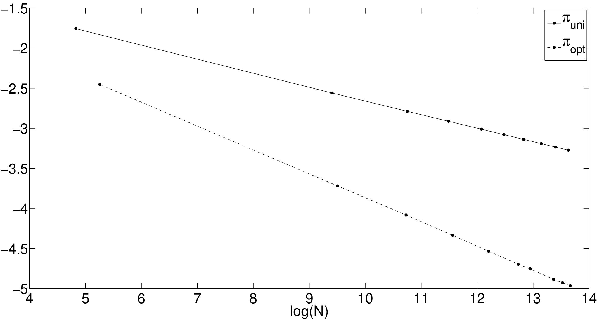
where 𝜶=(1/2,3/2)\boldsymbol{\alpha}=(1/2,3/2) and 𝐥=(1,2)\mathbf{l}=(1,2). Then X∈ℬ𝐥𝜶​([0,1]3,c⁡(⋅))X\in{\cal B}_{\mathbf{l}}^{\boldsymbol{\alpha}}([0,1]^{3},c(\cdot)), with c⁡(𝐭)=(1,1),𝐭∈[0,1]3c(\mathbf{t})=(1,1),\,\mathbf{t}\in[0,1]^{3}, k=2k=2, 𝜶∗=(1/2,3/2,3/2)\boldsymbol{\alpha}^{*}=(1/2,3/2,3/2). We compare behavior of eN​(hu​n​i,πu​n​i)e_{N}(h_{uni},\pi_{uni}) and eN​(hu​n​i,πo​p​t)e_{N}(h_{uni},\pi_{opt}), where πo​p​t\pi_{opt} given by Theorem 2. Observe that by using the asymptotically optimal intercomponent distribution, we obtain a gain in the rate of approximation. Figure 1 shows the (fitted) values of the squared IMSEs eN2​(hu​n​i,πu​n​i)e_{N}^{2}(h_{uni},\pi_{uni}) and eN2​(hu​n​i,πo​p​t)e_{N}^{2}(h_{uni},\pi_{opt}) in a log-log scale. In such scale, the slopes of fitted lines correspond to the rates of approximation.
Refer to caption
Figure 1: The (fitted) plots of eN2​(hu​n​i,πu​n​i)e_{N}^{2}(h_{uni},\pi_{uni}) (solid line), eN2​(hu​n​i,πo​p​t)e_{N}^{2}(h_{uni},\pi_{opt}) (dash line) versus NN in a log-log scale.

These plots represent the following asymptotic behavior:

eN2​(hu​n​i,πu​n​i)\displaystyle e_{N}^{2}(h_{uni},\pi_{uni}) ∼0.3667N−1/6+0.0935N−1/2∼0.3667N−1/6,\displaystyle\sim 0.3667N^{-1/6}+0.0935N^{-1/2}\sim 0.3667N^{-1/6},
eN2​(hu​n​i,πo​p​t)\displaystyle e_{N}^{2}(h_{uni},\pi_{opt}) ∼0.4245N−3/10\displaystyle\sim 0.4245N^{-3/10} as ​N→∞.\displaystyle\mbox{ as }N\to\infty.

Example 5. Let 𝒟=[0,1]2{\cal D}=[0,1]^{2} and define X⁡(𝐭)=X⁡(t1,t2)X(\mathbf{t})=X(t_{1},t_{2}) to be a zero mean Gaussian field with covariance function

Cov⁡(X⁡(𝐭),X⁡(𝐬))=1(‖𝐭‖2+0.1)​1(‖𝐬‖2+0.1)​exp⁡(−‖𝐭−𝐬‖).\mathrm{Cov}(X(\mathbf{t}),X(\mathbf{s}))=\frac{1}{(||\mathbf{t}||^{2}+0.1)}\frac{1}{(||\mathbf{s}||^{2}+0.1)}\exp(-||\mathbf{t-s}||).

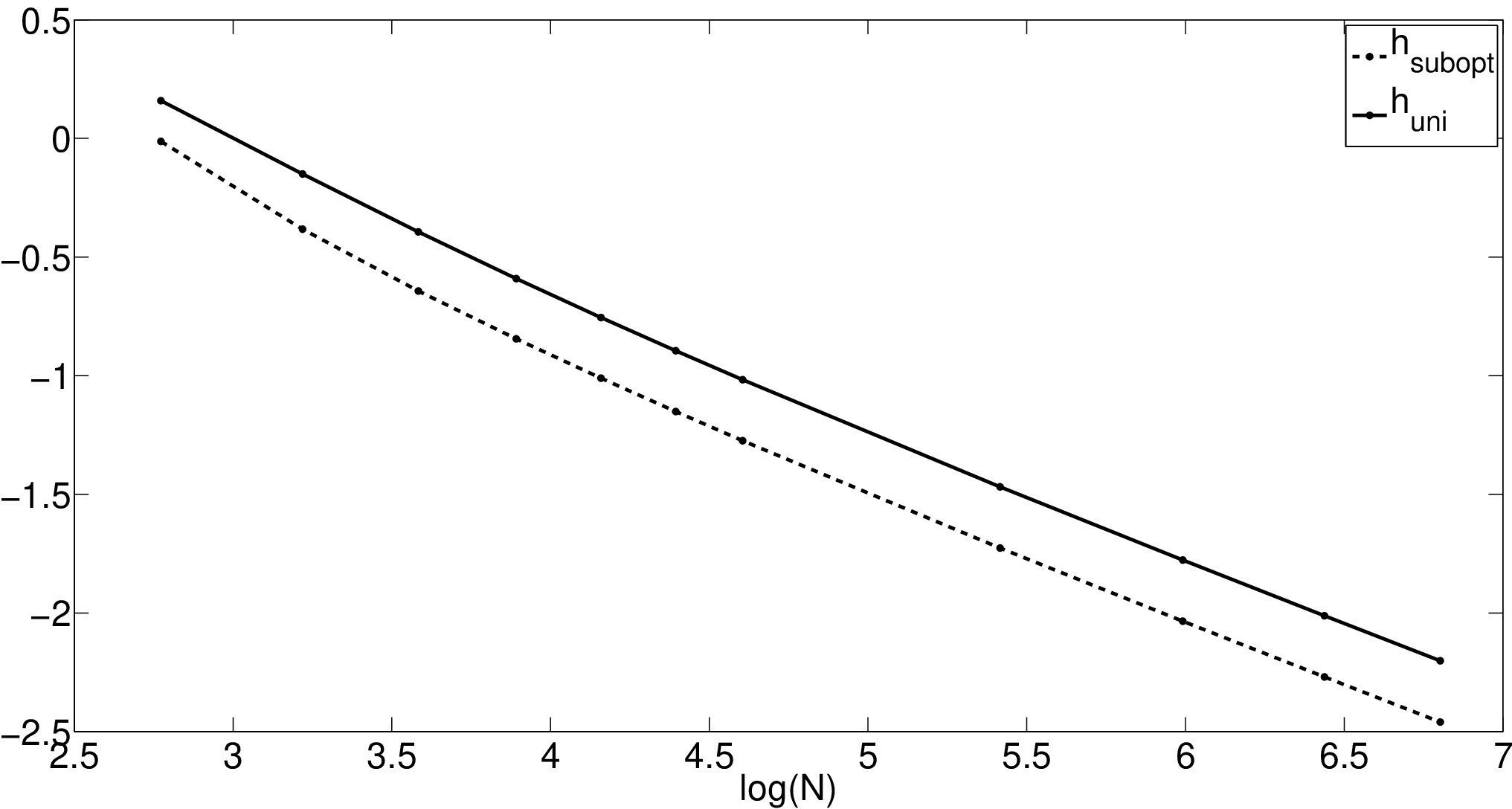
Then X∈ℬ𝐥𝜶​([0,1]2,c⁡(⋅))X\in{\cal B}_{\mathbf{l}}^{\boldsymbol{\alpha}}([0,1]^{2},c(\cdot)) with c⁡(𝐭)=c1​(𝐭)=2/(‖𝐭‖2+0.1)2,𝐭∈[0,1]2c(\mathbf{t})=c_{1}(\mathbf{t})=2/(||\mathbf{t}||^{2}+0.1)^{2},\,\mathbf{t}\in[0,1]^{2}, 𝜶=1\boldsymbol{\alpha}=1, 𝜶∗=(1,1)\boldsymbol{\alpha}^{*}=(1,1), 𝐥=2\mathbf{l}=2, and k=1k=1. The field has one component, hence the uniform interdimensional knot distribution is used. Theorem 2 provides the formula for the suboptimal withincomponent density. Figure 2(a) shows the (fitted) values of the squared IMSEs eN2​(hu​n​i,πu​n​i)e_{N}^{2}(h_{uni},\pi_{uni}) and eN2​(hs​u​b​o​p​t,πu​n​i)e_{N}^{2}(h_{subopt},\pi_{uni}). Figure 2(b) demonstrates the convergence of the scaled squared approximation error N0.5​eN2​(hs​u​b​o​p​t,πu​n​i)N^{0.5}e_{N}^{2}(h_{subopt},\pi_{uni}) to the asymptotic constant obtained in Theorem 1.
Refer to caption Refer to caption
(a) (b)
Figure 2: (a) The (fitted) plots of eN2​(hu​n​i,πu​n​i)e_{N}^{2}(h_{uni},\pi_{uni}) (dashed line) and eN2​(hs​u​b​o​p​t,πu​n​i)e_{N}^{2}(h_{subopt},\pi_{uni}) (solid line) versus NN in a log-log scale. (b) The convergence of N0.5​eN2​(hs​u​b​o​p​t,πu​n​i)N^{0.5}e_{N}^{2}(h_{subopt},\pi_{uni}) (solid line) to the asymptotic constant (dashed line).

Note that utilizing the suboptimal withincomponent density leads to a significant reduction of the asymptotic constant, as compared to the uniform withincomponent knot distribution.

4 Proofs

Proof of Theorem 1. First we investigate the asymptotic behavior of the approximation error eN​(𝐭):=||X⁡(𝐭)−XN​(𝐭)||e_{N}(\mathbf{t}):=\left|\left|\,X(\mathbf{t})-X_{N}(\mathbf{t})\,\right|\right| for any 𝐭∈𝒟𝐢\mathbf{t}\in{\cal D}_{\mathbf{i}}, 𝐢∈𝐈\mathbf{i}\in\mathbf{I}, where 𝐈:={𝐢=(i1,…,id)\mathbf{I}:=\{\mathbf{i}=(i_{1},\ldots,i_{d}), 0≤ik≤nk∗−10\leq i_{k}\leq n_{k}^{*}-1, k=1,…,d}k=1,\ldots,d\}, when the number of knots NN tends to infinity. Further, we find the asymptotic form of the IMSE

eN:=(∫𝒟eN​(𝐭)2​𝑑𝐭)1/2e_{N}:=\left(\int_{\cal D}e_{N}(\mathbf{t})^{2}d\mathbf{t}\right)^{1/2}

for any positive continuous densities h1​(⋅),…,hk​(⋅)h_{1}(\cdot),\ldots,h_{k}(\cdot). We start by observing that

eN​(𝐭)2\displaystyle e_{N}(\mathbf{t})^{2}\!\! =\displaystyle= E​(X⁡(𝐭)−XN​(𝐭))2=E​(E𝜼​(X⁡(𝐭𝐢+𝐫𝐢∗𝜼)−X⁡(𝐭)))2\displaystyle\!\!\!\mathrm{E}(X(\mathbf{t})-X_{N}(\mathbf{t}))^{2}=\mathrm{E}(\mathrm{E}_{\boldsymbol{\eta}}(X(\mathbf{t}_{\mathbf{i}}+\mathbf{r}_{\mathbf{i}}\!\!\ast\!\!{\boldsymbol{\eta}})-X(\mathbf{t})))^{2} (9)
=\displaystyle= E𝜼,𝝃​E​((X⁡(𝐭𝐢+𝐫𝐢∗𝜼)−X⁡(𝐭))​(X⁡(𝐭𝐢+𝐫𝐢∗𝝃)−X⁡(𝐭)))\displaystyle\!\!\!\mathrm{E}_{\boldsymbol{\eta},\boldsymbol{\xi}}\mathrm{E}\left(\left(X(\mathbf{t}_{\mathbf{i}}+\mathbf{r}_{\mathbf{i}}\!\!\ast\!\!{\boldsymbol{\eta}})-X(\mathbf{t})\right)\left(X(\mathbf{t}_{\mathbf{i}}+\mathbf{r}_{\mathbf{i}}\!\!\ast\!\!{\boldsymbol{\xi}})-X(\mathbf{t})\right)\right)
=\displaystyle= 12​E𝜼,𝝃​E​((X⁡(𝐭𝐢+𝐫𝐢∗𝜼)−X⁡(𝐭))2+(X⁡(𝐭𝐢+𝐫𝐢∗𝝃)−X⁡(𝐭))2−(X⁡(𝐭𝐢+𝐫𝐢∗𝜼)−X⁡(𝐭𝐢+𝐫𝐢∗𝝃))2),\displaystyle\!\!\!\frac{1}{2}\mathrm{E}_{\boldsymbol{\eta},\boldsymbol{\xi}}\mathrm{E}\left((X(\mathbf{t}_{\mathbf{i}}+\mathbf{r}_{\mathbf{i}}\!\ast\!\boldsymbol{\eta})\!\!-\!\!X(\mathbf{t}))^{2}\!\!+\!\!(X(\mathbf{t}_{\mathbf{i}}+\mathbf{r}_{\mathbf{i}}\!\ast\!\boldsymbol{\xi})\!\!-\!\!X(\mathbf{t}))^{2}\!-\!(X(\mathbf{t}_{\mathbf{i}}+\mathbf{r}_{\mathbf{i}}\!\ast\!\boldsymbol{\eta})\!\!-\!\!X(\mathbf{t}_{\mathbf{i}}+\mathbf{r}_{\mathbf{i}}\!\ast\!\boldsymbol{\xi}))^{2}\right),

where 𝝃\boldsymbol{\xi} is an independent copy of 𝜼\boldsymbol{\eta}. Further, the property (2) together with the uniform continuity and positiveness of local stationarity functions c1​(⋅),…,ck​(⋅)c_{1}(\cdot),\ldots,c_{k}(\cdot) imply that

eN​(𝐭)2=12​(∑j=1kcj​(𝐭𝐢)​E𝜼,𝝃​(||𝐫𝐢j∗(𝜼j−𝐬j)||αj+||𝐫𝐢j∗(𝝃j−𝐬j)||αj−||𝐫𝐢j∗(𝜼j−𝝃j)||αj))​(1+qN,𝐢​(𝐭)),e_{N}(\mathbf{t})^{2}=\frac{1}{2}\left(\sum_{j=1}^{k}c_{j}(\mathbf{t}_{\mathbf{i}})\mathrm{E}_{\boldsymbol{\eta},\boldsymbol{\xi}}\left(\left|\left|\,\mathbf{r}^{j}_{\mathbf{i}}\!\ast\!(\boldsymbol{\eta}^{j}-\mathbf{s}^{j})\,\right|\right|^{\alpha_{j}}\!\!\!\!+\left|\left|\,\mathbf{r}^{j}_{\mathbf{i}}\!\ast\!(\boldsymbol{\xi}^{j}-\mathbf{s}^{j})\,\right|\right|^{\alpha_{j}}\!\!\!\!-\left|\left|\,\mathbf{r}^{j}_{\mathbf{i}}\!\ast\!(\boldsymbol{\eta}^{j}-\boldsymbol{\xi}^{j})\,\right|\right|^{\alpha_{j}}\right)\right)(1+q_{N,\mathbf{i}}(\mathbf{t})), (10)

where εN:=max⁡{|qN,𝐢​(𝐭)|,𝐭∈𝒟𝐢,𝐢∈𝐈}=o⁡(1)\varepsilon_{N}:=\max\{|q_{N,\mathbf{i}}(\mathbf{t})|,\mathbf{t}\in{\cal D}_{\mathbf{i}},\mathbf{i}\in\mathbf{I}\}=\mathrm{o}(1) as N→∞N\to\infty (Seleznjev, 2000, cf.). It follows from the definition and the mean (integral) value theorem that

𝐫𝐢=(1h1∗​(w1,i1)​n1∗,1h2∗​(w2,i2)​n2∗,…,1hd∗​(wd,id)​nd∗),wj,ij∈[tj,ij,tj,ij+1],j=1,…,d.\mathbf{r}_{\mathbf{i}}=\left(\frac{1}{h_{1}^{*}(w_{1,i_{1}})n_{1}^{*}},\frac{1}{h_{2}^{*}(w_{2,i_{2}})n_{2}^{*}},\ldots,\frac{1}{h_{d}^{*}(w_{d,i_{d}})n_{d}^{*}}\right),\quad w_{j,i_{j}}\in[t_{j,i_{j}},t_{j,i_{j}+1}],\,j=1,\ldots,d.

Denote by 𝐰𝐢:=(w1,i1,…,wd,id)\mathbf{w}_{\mathbf{i}}:=(w_{1,i_{1}},\ldots,w_{d,i_{d}}). Now the definition of c​R​S​(h,π,𝐥)cRS(h,\pi,\mathbf{l}) implies

𝐫𝐢j=(1nj​hj​(wLj−1+1,iLj−1+1),…,1nj​hj​(wLj,iLj))=1njHj(𝐰𝐢j),j=1,…,k,\mathbf{r}_{\mathbf{i}}^{j}=\left(\frac{1}{n_{j}h_{j}(w_{L_{j-1}+1,i_{L_{j-1}+1}})},\ldots,\frac{1}{n_{j}h_{j}(w_{L_{j},i_{L_{j}}})}\right)=\frac{1}{n_{j}}H_{j}(\mathbf{w}_{\mathbf{i}}^{j}),\quad j=1,\ldots,k,

where Hj​(𝐭j):=(1/hj​(tLj−1+1),…,1/hj​(tLj))H_{j}(\mathbf{t}^{j}):=(1/h_{j}(t_{L_{j-1}+1}),\ldots,1/h_{j}(t_{L_{j}})), j=1,…,kj=1,\ldots,k. Consequently,

eN​(𝐭)2\displaystyle e_{N}(\mathbf{t})^{2} =\displaystyle= 12​(∑j=1knj−αj​cj​(𝐭𝐢)​Eη,ξ​(‖Hj​(𝐰𝐢j)∗(𝜼j−𝐬j)‖αj+‖Hj​(𝐰𝐢j)∗(𝝃j−𝐬j)‖αjCLOSECLOSE\displaystyle\frac{1}{2}\Bigg(\sum_{j=1}^{k}n_{j}^{-\alpha_{j}}c_{j}(\mathbf{t}_{\mathbf{i}})\mathrm{E}_{\eta,\xi}\Big(||H_{j}(\mathbf{w}^{j}_{\mathbf{i}})\ast(\boldsymbol{\eta}^{j}-\mathbf{s}^{j})||^{\alpha_{j}}+||H_{j}(\mathbf{w}^{j}_{\mathbf{i}})\ast(\boldsymbol{\xi}^{j}-\mathbf{s}^{j})||^{\alpha_{j}}
OPENOPEN−‖Hj​(𝐰𝐢j)∗(𝜼j−𝝃j)‖αj))​(1+o⁡(1)) as ​N→∞.\displaystyle\qquad\qquad-||H_{j}(\mathbf{w}^{j}_{\mathbf{i}})\ast(\boldsymbol{\eta}^{j}-{\boldsymbol{\xi}}^{j})||^{\alpha_{j}}\Big)\Bigg)(1+\mathrm{o}(1))\quad\mbox{ as }N\to\infty.

Applying the uniform continuity of h⁡(⋅)h(\cdot) yields

eN​(t)2\displaystyle e_{N}(t)^{2} =12​(∑j=1knj−αj​cj​(𝐭𝐢)​Eη,ξ​(‖Hj​(𝐭𝐢j)∗(𝜼j−𝐬j)‖αj+‖Hj​(𝐭𝐢j)∗(𝝃j−𝐬j)‖αjCLOSECLOSE\displaystyle=\frac{1}{2}\Bigg(\sum_{j=1}^{k}n_{j}^{-\alpha_{j}}c_{j}(\mathbf{t_{i}})\mathrm{E}_{\eta,\xi}\Big(||H_{j}(\mathbf{t}^{j}_{\mathbf{i}})\ast(\boldsymbol{\eta}^{j}-\mathbf{s}^{j})||^{\alpha_{j}}+||H_{j}(\mathbf{t}^{j}_{\mathbf{i}})\ast(\boldsymbol{\xi}^{j}-\mathbf{s}^{j})||^{\alpha_{j}}
OPENOPEN−‖Hj​(𝐭𝐢j)∗(𝜼j−𝝃j)‖αj))​(1+o⁡(1))\displaystyle-||H_{j}(\mathbf{t}^{j}_{\mathbf{i}})\ast(\boldsymbol{\eta}^{j}-{\boldsymbol{\xi}}^{j})||^{\alpha_{j}}\Big)\Bigg)(1+\mathrm{o}(1))
=(∑j=1knj−αjcj(𝐭𝐢)Cαj,lj(𝐬j;Hj(𝐭j𝐢)))(1+o(1)) as N→∞,\displaystyle=\Bigg(\sum_{j=1}^{k}n_{j}^{-\alpha_{j}}c_{j}(\mathbf{t_{i}})C_{\alpha_{j},l_{j}}(\mathbf{s}^{j};H_{j}(\mathbf{t}^{j}_{\mathbf{i}}))\Bigg)(1+\mathrm{o}(1))\quad\mbox{ as }N\to\infty,

where

Cαj,lj​(𝐬j,Hj​(𝐭𝐢j)):=\displaystyle C_{\alpha_{j},l_{j}}(\mathbf{s}^{j};H_{j}(\mathbf{t}^{j}_{\mathbf{i}})):= 12​E𝜼,𝝃​(‖Hj​(𝐭𝐢j)∗(𝜼j−𝐬j)‖αj+‖Hj​(𝐭𝐢j)∗(𝝃j−𝐬j)‖αj−‖Hj​(𝐭𝐢j)∗(𝜼j−𝝃j)‖αj)\displaystyle\frac{1}{2}\mathrm{E}_{\boldsymbol{\eta},\boldsymbol{\xi}}\Big(||H_{j}(\mathbf{t}^{j}_{\mathbf{i}})\ast(\boldsymbol{\eta}^{j}-\mathbf{s}^{j})||^{\alpha_{j}}+||H_{j}(\mathbf{t}^{j}_{\mathbf{i}})\ast(\boldsymbol{\xi}^{j}-\mathbf{s}^{j})||^{\alpha_{j}}-||H_{j}(\mathbf{t}^{j}_{\mathbf{i}})\ast(\boldsymbol{\eta}^{j}-{\boldsymbol{\xi}}^{j})||^{\alpha_{j}}\Big)
=\displaystyle= ||Bαj,lj​(Hj​(𝐭𝐢j)∗𝐬j)−E𝜼​Bαj,lj​(Hj​(𝐭𝐢j)∗𝜼j)||22.\displaystyle\left|\left|\,B_{\alpha_{j},l_{j}}(H_{j}(\mathbf{t}^{j}_{\mathbf{i}})\ast\mathbf{s}^{j})-\mathrm{E}_{\boldsymbol{\eta}}B_{\alpha_{j},l_{j}}(H_{j}(\mathbf{t}^{j}_{\mathbf{i}})\!\ast\!\boldsymbol{\eta}^{j})\,\right|\right|^{2}_{2}.

Let 𝒟𝐢=𝒟𝐢1×⋯×𝒟𝐢k{\cal D}_{\mathbf{i}}={\cal D}_{\mathbf{i}}^{1}\times\cdots\times{\cal D}_{\mathbf{i}}^{k} and denote by |𝒟𝐢||{\cal D}_{\mathbf{i}}| the volume of hyperrectangle 𝒟𝐢{\cal D}_{\mathbf{i}}. Then

eN2\displaystyle e_{N}^{2} =∑𝐢∈𝐈∫𝒟𝐢eN​(𝐭)2​d𝐭=(∑𝐢∈𝐈∫𝒟𝐢∑j=1knj−αj​cj​(𝐭𝐢)​Cαj,lj​(𝐬j,Hj​(𝐭𝐢j))​d𝐭)​(1+o⁡(1))\displaystyle=\sum_{\mathbf{i}\in\mathbf{I}}\int_{{\cal D}_{\mathbf{i}}}e_{N}(\mathbf{t})^{2}d\mathbf{t}=\Bigg(\sum_{\mathbf{i}\in\mathbf{I}}\int_{{\cal D}_{\mathbf{i}}}\sum_{j=1}^{k}n_{j}^{-\alpha_{j}}c_{j}(\mathbf{t_{i}})C_{\alpha_{j},l_{j}}(\mathbf{s}^{j};H_{j}(\mathbf{t}^{j}_{\mathbf{i}}))d\mathbf{t}\Bigg)(1+\mathrm{o}(1))
=(∑𝐢∈𝐈∑j=1knj−αj​cj​(𝐭𝐢)​∫𝒟jCαj,lj​(𝐬j,Hj​(𝐭𝐢j))​d​𝐬j​|𝒟𝐢|)​(1+o⁡(1))\displaystyle=\Bigg(\sum_{\mathbf{i}\in\mathbf{I}}\sum_{j=1}^{k}n_{j}^{-\alpha_{j}}c_{j}(\mathbf{t_{i}})\int_{{\cal D}^{j}}C_{\alpha_{j},l_{j}}(\mathbf{s}^{j};H_{j}(\mathbf{t}^{j}_{\mathbf{i}}))d\mathbf{s}^{j}|{\cal D}_{\mathbf{i}}|\Bigg)(1+\mathrm{o}(1))
=(∑j=1knj−αj​∑𝐢∈𝐈cj​(𝐭𝐢)​bαj,lj​(Hj​(𝐭𝐢j))​|𝒟𝐢|)​(1+o⁡(1))​ as ​N→∞.\displaystyle=\Bigg(\sum_{j=1}^{k}n_{j}^{-\alpha_{j}}\sum_{\mathbf{i}\in\mathbf{I}}c_{j}(\mathbf{t_{i}})b_{\alpha_{j},l_{j}}(H_{j}(\mathbf{t}^{j}_{\mathbf{i}}))|{\cal D}_{\mathbf{i}}|\Bigg)(1+\mathrm{o}(1))\mbox{ as }N\to\infty.

Now the Riemann integrability of the functions cj​(𝐭)​bαj,lj​(Hj​(𝐭j))c_{j}(\mathbf{t})b_{\alpha_{j},l_{j}}(H_{j}(\mathbf{t}^{j})), j=1,…,kj=1,\ldots,k, gives

eN2\displaystyle e_{N}^{2} =(∑j=1knj−αj∫𝒟cj(𝐭)bαj,lj(Hj(𝐭j))d𝐭)(1+o(1))=(∑j=1kvjnjαj)(1+o(1)) as N→∞.\displaystyle=\Bigg(\sum_{j=1}^{k}n_{j}^{-\alpha_{j}}\int_{\cal D}c_{j}(\mathbf{t})b_{\alpha_{j},l_{j}}(H_{j}(\mathbf{t}^{j}))d\mathbf{t}\Bigg)(1+\mathrm{o}(1))=\Bigg(\sum_{j=1}^{k}\frac{v_{j}}{n_{j}^{\alpha_{j}}}\Bigg)(1+\mathrm{o}(1))\quad\mbox{ as }N\to\infty.

Note that for any 𝐮∈ℝ+m\mathbf{u}\in\mathbb{R}^{m}_{+}, bβ,m​(𝐮)>0b_{\beta,m}(\mathbf{u})>0, otherwise the fractional Brownian field is degenerated (Seleznjev, 2000, cf.). Consequently, vj>0v_{j}>0, j=1,…,kj=1,\ldots,k. This completes the proof.

Proof of Theorem 2. Note that by the inequality for the arithmetic and geometric means,

1k​∑j=1kvjnjαj≥(∏j=1kvjnjαj)1/k\frac{1}{k}\sum_{j=1}^{k}\frac{v_{j}}{n_{j}^{\alpha_{j}}}\geq\left(\prod_{j=1}^{k}\frac{v_{j}}{n_{j}^{\alpha_{j}}}\right)^{1/k}

with equality if only if

ν−1=vjnjαj,j=1,…,k.\nu^{-1}=\frac{v_{j}}{n_{j}^{\alpha_{j}}},\quad j=1,\ldots,k.

Hence, the equality is attained for n~j=(ν​vj)1/αj\tilde{n}_{j}=(\nu v_{j})^{1/\alpha_{j}}, j=1,…,kj=1,\ldots,k. Let

nj=⌈n~j⌉∼(ν​vj)1/αj​ as ​N→∞.n_{j}=\left\lceil\tilde{n}_{j}\right\rceil\sim\left({\nu}{v_{j}}\right)^{1/\alpha_{j}}\mbox{ as }N\to\infty. (11)

The total number of observations satisfies

N=(n1∗+1)⋯(nd∗+1)∼∏i=1dni∗=∏j=1knjlj=M as N→∞.N=(n_{1}^{*}+1)\cdots(n_{d}^{*}+1)\sim\prod_{i=1}^{d}n_{i}^{*}=\prod_{j=1}^{k}n_{j}^{l_{j}}=M\quad\mbox{ as }N\to\infty.

This implies that for the asymptotically optimal intercomponent knot distribution

N∼M∼ν1/ρ​∏j=1kvjlj/αj,N\sim M\sim\nu^{1/\rho}\prod_{j=1}^{k}{v_{j}^{l_{j}/\alpha_{j}}},

and therefore,

ν∼Nρ​κ−ρ​ as ​N→∞.\nu\sim{N^{\rho}}{\kappa^{-\rho}}\mbox{ as }N\to\infty.

By equation (11), the asymptotically optimal intercomponent knot distribution is

nj∼Nρ/αj​vj1/αjκρ/αj as N→∞,j=1,…,k.n_{j}\sim\frac{N^{\rho/\alpha_{j}}v_{j}^{1/\alpha_{j}}}{\kappa^{\rho/\alpha_{j}}}\mbox{ as }N\to\infty,\quad j=1,\ldots,k.

Moreover, with such chosen knot distribution, the equality in (5) is attained asymptotically. This completes the proof.

Proof of Proposition 1. The proof is a straightforward implication of the assumptions and equation (10). The exact constant and the expression for the optimal density are due to Seleznjev (2000).

Proof of Proposition 2. The first steps of the proof repeat those of Theorem 1. By (10), we have

eN​(𝐭)2\displaystyle e_{N}(\mathbf{t})^{2} =12​(∑j=1kcj​(𝐭𝐢)​E𝜼,𝝃​(||𝐫𝐢j∗(𝜼j−𝐬j)||αj+||𝐫𝐢j∗(𝝃j−𝐬j)||αj−||𝐫𝐢j∗(𝜼j−𝝃j)||αj))​(1+o⁡(1))\displaystyle=\frac{1}{2}\Bigg(\sum_{j=1}^{k}c_{j}(\mathbf{t}_{\mathbf{i}})\mathrm{E}_{\boldsymbol{\eta},\boldsymbol{\xi}}\left(\left|\left|\,\mathbf{r}^{j}_{\mathbf{i}}\!\ast\!(\boldsymbol{\eta}^{j}-\mathbf{s}^{j})\,\right|\right|^{\alpha_{j}}+\left|\left|\,\mathbf{r}^{j}_{\mathbf{i}}\!\ast\!(\boldsymbol{\xi}^{j}-\mathbf{s}^{j})\,\right|\right|^{\alpha_{j}}-\left|\left|\,\mathbf{r}^{j}_{\mathbf{i}}\!\ast\!(\boldsymbol{\eta}^{j}-\boldsymbol{\xi}^{j})\,\right|\right|^{\alpha_{j}}\right)\Bigg)(1+\mathrm{o}(1))
≤12​(∑j=1kcj​(𝐭𝐢)​E𝜼,𝝃​(||𝐫𝐢j∗(𝜼j−𝐬j)||αj+||𝐫𝐢j∗(𝝃j−𝐬j)||αj))​(1+o⁡(1))\displaystyle\leq\frac{1}{2}\Bigg(\sum_{j=1}^{k}c_{j}(\mathbf{t}_{\mathbf{i}})\mathrm{E}_{\boldsymbol{\eta},\boldsymbol{\xi}}\left(\left|\left|\,\mathbf{r}^{j}_{\mathbf{i}}\!\ast\!(\boldsymbol{\eta}^{j}-\mathbf{s}^{j})\,\right|\right|^{\alpha_{j}}+\left|\left|\,\mathbf{r}^{j}_{\mathbf{i}}\!\ast\!(\boldsymbol{\xi}^{j}-\mathbf{s}^{j})\,\right|\right|^{\alpha_{j}}\right)\Bigg)(1+\mathrm{o}(1))
=(∑j=1kcj​(𝐭𝐢)​E𝜼​(||𝐫𝐢j∗(𝜼j−𝐬j)||αj))​(1+o⁡(1))​ as ​N→∞.\displaystyle=\Bigg(\sum_{j=1}^{k}c_{j}(\mathbf{t}_{\mathbf{i}})\mathrm{E}_{\boldsymbol{\eta}}\left(\left|\left|\,\mathbf{r}^{j}_{\mathbf{i}}\!\ast\!(\boldsymbol{\eta}^{j}-\mathbf{s}^{j})\,\right|\right|^{\alpha_{j}}\right)\Bigg)(1+\mathrm{o}(1))\mbox{ as }N\to\infty.

For any nonnegative numbers a1,…,aka_{1},\ldots,a_{k} and any α∈ℝ+\alpha\in\mathbb{R_{+}}, the inequality

(∑i=1kai)α≤kα​∑i=1kaiα\left(\sum_{i=1}^{k}a_{i}\right)^{\alpha}\leq k^{\alpha}\sum_{i=1}^{k}a_{i}^{\alpha} (12)

holds, and consequently,

eN​(𝐭)2\displaystyle e_{N}(\mathbf{t})^{2} ≤(∑j=1kcj​(𝐭𝐢)​ljαj/2​∑m=Lj−1+1LjE𝜼​(r𝐢,m​|ηm−sm|)αj)​(1+o⁡(1))\displaystyle\leq\Bigg(\sum_{j=1}^{k}c_{j}(\mathbf{t_{i}})l_{j}^{\alpha_{j}/2}\sum_{m=L_{j-1}+1}^{L_{j}}\mathrm{E}_{\boldsymbol{\eta}}(r_{\mathbf{i},m}|\eta_{m}-s_{m}|)^{\alpha_{j}}\Bigg)(1+\mathrm{o}(1))
=(∑j=1kcj​(𝐭𝐢)​ljαj/2​∑m=Lj−1+1Ljr𝐢,mαj​((1−sm)αj​sm+(1−sm)​smαj))​(1+o⁡(1)).\displaystyle=\Bigg(\sum_{j=1}^{k}c_{j}(\mathbf{t_{i}})l_{j}^{\alpha_{j}/2}\sum_{m=L_{j-1}+1}^{L_{j}}r_{\mathbf{i},m}^{\alpha_{j}}\left((1-s_{m})^{\alpha_{j}}s_{m}+(1-s_{m})s_{m}^{\alpha_{j}}\right)\Bigg)(1+\mathrm{o}(1)).

By the mean value theorem and the uniform continuity of withincomponent densities, we obtain

eN​(𝐭)2\displaystyle e_{N}(\mathbf{t})^{2} ≤(∑j=1kcj​(𝐭𝐢)​ljαj/2​nj−αj​∑m=Lj−1+1Lj(hj​(t𝐢,m))−αj​((1−sm)αj​sm+(1−sm)​smαj))​(1+o⁡(1))​ as ​N→∞.\displaystyle\leq\Bigg(\sum_{j=1}^{k}c_{j}(\mathbf{t_{i}})l_{j}^{\alpha_{j}/2}n_{j}^{-\alpha_{j}}\!\!\!\sum_{m=L_{j-1}+1}^{L_{j}}(h_{j}(t_{\mathbf{i},m}))^{-\alpha_{j}}\left((1-s_{m})^{\alpha_{j}}s_{m}+(1-s_{m})s_{m}^{\alpha_{j}}\right)\Bigg)(1+\mathrm{o}(1))\mbox{ as }N\to\infty.

Proceeding now to the calculation of the IMSE, we get

eN2\displaystyle e_{N}^{2} =∑𝐢∈𝐈∫𝒟𝐢eN​(𝐭)2​dt≤(∑𝐢∈𝐈∑j=1kcj​(𝐭𝐢)​ljαj/2​nj−αj​∑m=Lj−1+1Lj(hj​(t𝐢,m))−αj​2(αj+1)​(αj+2)​|𝒟𝐢|)​(1+o⁡(1)),\displaystyle=\sum_{\mathbf{i}\in\mathbf{I}}\int_{{\cal D}_{\mathbf{i}}}e_{N}(\mathbf{t})^{2}dt\leq\Bigg(\sum_{\mathbf{i}\in\mathbf{I}}\sum_{j=1}^{k}c_{j}(\mathbf{t_{i}})l_{j}^{\alpha_{j}/2}n_{j}^{-\alpha_{j}}\sum_{m=L_{j-1}+1}^{L_{j}}(h_{j}(t_{\mathbf{i},m}))^{-\alpha_{j}}\frac{2}{(\alpha_{j}+1)(\alpha_{j}+2)}|{\cal D}_{\mathbf{i}}|\Bigg)(1+\mathrm{o}(1)),

where

2(αj+1)​(αj+2)=∫01((1−s)αj​s+(1−s)​sαj)​𝑑s.\frac{2}{(\alpha_{j}+1)(\alpha_{j}+2)}=\int_{0}^{1}\left((1-s)^{\alpha_{j}}s+(1-s)s^{\alpha_{j}}\right)ds.

Now the Riemann integrability of cj​(𝐭)​hj​(tm)−αjc_{j}(\mathbf{t})h_{j}(t_{m})^{-\alpha_{j}}, j=1,…,kj=1,\ldots,k, together with the definition of integrated local stationarity functions imply that

eN2\displaystyle e_{N}^{2} ≤(∑j=1k1njαj​ljαj/2​(aαj+16)​∑m=Lj−1+1Lj∑𝐢∈𝐈cj​(𝐭𝐢)​(hj​(t𝐢,m))−αj​|𝒟𝐢|)​(1+o⁡(1))\displaystyle\leq\Bigg(\sum_{j=1}^{k}\frac{1}{n_{j}^{\alpha_{j}}}{l_{j}^{\alpha_{j}/2}}\left(a_{\alpha_{j}}+\frac{1}{6}\right)\sum_{m=L_{j-1}+1}^{L_{j}}\sum_{\mathbf{i}\in\mathbf{I}}c_{j}(\mathbf{t_{i}})(h_{j}(t_{\mathbf{i},m}))^{-\alpha_{j}}|{\cal D}_{\mathbf{i}}|\Bigg)(1+\mathrm{o}(1))
=(∑j=1k1njαj​ljαj/2​(aαj+16)​∑m=Lj−1+1Lj∫𝒟cj​(𝐭)​hj​(tm)−αj​dt)​(1+o⁡(1))\displaystyle=\Bigg(\sum_{j=1}^{k}\frac{1}{n_{j}^{\alpha_{j}}}{l_{j}^{\alpha_{j}/2}}\left(a_{\alpha_{j}}+\frac{1}{6}\right)\sum_{m=L_{j-1}+1}^{L_{j}}\int_{\cal D}c_{j}(\mathbf{t})h_{j}(t_{m})^{-\alpha_{j}}dt\Bigg)(1+\mathrm{o}(1))
=(∑j=1k1njαj​lj1+αj/2​(aαj+16)​∫01Cj​(tLj)​hj​(tLj)−αj​d​tLj)​(1+o⁡(1))​ as ​N→∞.\displaystyle=\Bigg(\sum_{j=1}^{k}\frac{1}{n_{j}^{\alpha_{j}}}{l_{j}^{1+\alpha_{j}/2}}\left(a_{\alpha_{j}}+\frac{1}{6}\right)\int_{0}^{1}C_{j}(t_{L_{j}})h_{j}(t_{L_{j}})^{-\alpha_{j}}dt_{L_{j}}\Bigg)(1+\mathrm{o}(1))\mbox{ as }N\to\infty.

The expression for the suboptimal density is due to Seleznjev (2000). This completes the proof.

Proof of Proposition 3. We start by proving (i)(i). Let X∈𝒞𝐥𝜶​([0,1]d,C)X\in{\cal C}^{\boldsymbol{\alpha}}_{\mathbf{l}}([0,1]^{d},C) and consider 𝐭∈𝒟𝐢\mathbf{t}\in{\cal D}_{\mathbf{i}}, 𝐢∈𝐈\mathbf{i}\in\mathbf{I}. Applying the Hölder condition (1) to equation (9) yields

eN​(𝐭)2\displaystyle e_{N}(\mathbf{t})^{2} =12​E𝜼,𝝃​E​((X⁡(𝐭𝐢+𝐫𝐢∗𝜼)−X⁡(𝐭))2+(X⁡(𝐭𝐢+𝐫𝐢∗𝝃)−X⁡(𝐭))2−(X⁡(𝐭𝐢+𝐫𝐢∗𝜼)−X⁡(𝐭𝐢+𝐫𝐢∗𝝃))2)\displaystyle=\frac{1}{2}\mathrm{E}_{\boldsymbol{\eta},\boldsymbol{\xi}}\mathrm{E}\left((X(\mathbf{t}_{\mathbf{i}}+\mathbf{r}_{\mathbf{i}}\!\ast\!\boldsymbol{\eta})-X(\mathbf{t}))^{2}\!\!+\!\!(X(\mathbf{t}_{\mathbf{i}}+\mathbf{r}_{\mathbf{i}}\!\ast\!\boldsymbol{\xi})-X(\mathbf{t}))^{2}\!-\!(X(\mathbf{t}_{\mathbf{i}}+\mathbf{r}_{\mathbf{i}}\!\ast\!\boldsymbol{\eta})-X(\mathbf{t}_{\mathbf{i}}+\mathbf{r}_{\mathbf{i}}\!\ast\!\boldsymbol{\xi}))^{2}\right)
≤C​E𝜼​||𝐫𝐢∗𝜼||𝜶=C​E𝜼​∑j=1k||𝐫𝐢j∗𝜼j||αj≤C​∑j=1kljαj/2​∑m=Lj−1+1LjE𝜼​(r𝐢,m​|ηm−sm|)αj,\displaystyle\leq C\mathrm{E}_{\boldsymbol{\eta}}\left|\left|\,\mathbf{r_{i}}\ast\boldsymbol{\eta}\,\right|\right|_{\boldsymbol{\alpha}}=C\mathrm{E}_{\boldsymbol{\eta}}\sum_{j=1}^{k}\left|\left|\,\mathbf{r_{i}}^{j}\ast\boldsymbol{\eta}^{j}\,\right|\right|^{\alpha_{j}}\leq C\sum_{j=1}^{k}l_{j}^{\alpha_{j}/2}\!\!\!\!\sum_{m=L_{j-1}+1}^{L_{j}}\mathrm{E}_{\boldsymbol{\eta}}\left({r}_{\mathbf{i},m}|\eta_{m}-s_{m}|\right)^{\alpha_{j}},

where the last inequality follows from (12). Furthermore, since maxs∈[0,1]⁡((1−s)αj​s+(1−s)​sαj)=2−αj\max_{s\in[0,1]}\left((1-s)^{\alpha_{j}}s+(1-s)s^{\alpha_{j}}\right)=2^{-\alpha_{j}}, we obtain

eN​(𝐭)2\displaystyle e_{N}(\mathbf{t})^{2} ≤C​∑j=1kljαj/2​∑m=Lj−1+1Ljr𝐢,mαj​((1−sm)αj​sm+(1−sm)​smαj)≤∑j=1k2−αj​ljαj/2​∑m=Lj−1+1Ljr𝐢,mαj.\displaystyle\leq C\sum_{j=1}^{k}l_{j}^{\alpha_{j}/2}\!\!\!\!\sum_{m=L_{j-1}+1}^{L_{j}}r_{\mathbf{i},m}^{\alpha_{j}}\left((1-s_{m})^{\alpha_{j}}s_{m}+(1-s_{m})s_{m}^{\alpha_{j}}\right)\leq\sum_{j=1}^{k}2^{-\alpha_{j}}l_{j}^{\alpha_{j}/2}\!\!\!\!\sum_{m=L_{j-1}+1}^{L_{j}}r_{\mathbf{i},m}^{\alpha_{j}}.

By the regularity of the generating densities, we have that r𝐢,m≤1/(nm∗mins∈[0,1]hm∗(s)),𝐢∈𝐈,m=1,…,dr_{\mathbf{i},m}\leq 1/(n_{m}^{*}\min_{s\in[0,1]}h^{*}_{m}(s)),\mathbf{i}\in\mathbf{I},m=1,\ldots,d. Moreover, the definition of c​R​S​(h,π,𝐥)cRS(h,\pi,\mathbf{l}) implies the following uniform bound for the squared approximation accuracy

||X−XN||∞2=max𝐭∈𝒟⁡eN2​(𝐭)≤C​∑j=1k2−αj​lj1+αj/2​(Djnj)αj,\left|\left|\,X-X_{N}\,\right|\right|^{2}_{\infty}=\max_{\mathbf{t}\in{\cal D}}e_{N}^{2}(\mathbf{t})\leq C\sum_{j=1}^{k}2^{-\alpha_{j}}l_{j}^{1+\alpha_{j}/2}\left(\frac{D_{j}}{n_{j}}\right)^{\alpha_{j}},\\

with Dj=1/mins∈[0,1]⁡hj​(s)D_{j}=1/\min_{s\in[0,1]}h_{j}(s), j=1,…,kj=1,\ldots,k. Finally, we obtain the required assertion

||X−XN||∞≤C​∑j=1kcjnjαj/2,\left|\left|\,X-X_{N}\,\right|\right|_{\infty}\leq\sqrt{C}\sum_{j=1}^{k}\frac{c_{j}}{n_{j}^{\alpha_{j}/2}},

where cj2:=2−αj​lj1+αj/2​Djαj>0c_{j}^{2}:=2^{-\alpha_{j}}l_{j}^{1+\alpha_{j}/2}D_{j}^{\alpha_{j}}>0, j=1,…,kj=1,\ldots,k.

For the smooth case, we use the multivariate Taylor formula to obtain the following representation of the deviation field

δn(𝐭):=X(𝐭)−XN(𝐭)=E𝜼(∫01∑j=1dXj′(𝐭𝐢+u𝐫𝐢∗(𝜼−𝐬))r𝐢,j(ηj−sj)du),𝐭∈𝒟𝐢,𝐭=𝐭𝐢+𝐬∗𝐫𝐢,\displaystyle\delta_{n}(\mathbf{t}):=X(\mathbf{t})-X_{N}(\mathbf{t})=\mathrm{E}_{\boldsymbol{\eta}}\left(\int_{0}^{1}\sum_{j=1}^{d}X_{j}^{\prime}(\mathbf{t_{i}}+u\,\mathbf{r_{i}}\ast(\boldsymbol{\eta}-\mathbf{s})){r}_{\mathbf{i},j}(\eta_{j}-s_{j})du\right),\quad\mathbf{t}\in{\cal D}_{\mathbf{i}},\,\mathbf{t}=\mathbf{t_{i}}+\mathbf{s}\ast\mathbf{r_{i}},

where 𝜼=(η1,…,ηd)\boldsymbol{\eta}=(\eta_{1},\ldots,\eta_{d}) and η1,…,ηd\eta_{1},\ldots,\eta_{d} are independent Bernoulli random variables, ηj∈Be(sj),j=1,…,d\eta_{j}\in Be(s_{j}),\,j=1,\ldots,d. Introducing an auxiliary uniform random variable U∈𝒰⁡(0,1)U\in\mathscr{U}(0,1) we get

δn​(𝐭)\displaystyle\delta_{n}(\mathbf{t}) =∑j=1dE𝜼,U​(Xj′​(𝐭𝐢+U⁡(𝜼−𝐬)∗𝐫𝐢)​r𝐢,j​(ηj−sj))\displaystyle=\sum_{j=1}^{d}\mathrm{E}_{\boldsymbol{\eta},U}\left(X_{j}^{\prime}(\mathbf{t_{i}}+U(\boldsymbol{\eta}-\mathbf{s})\!\ast\!\mathbf{r_{i}}){r}_{\mathbf{i},j}(\eta_{j}-s_{j})\right)
=∑j=1dE𝜼,U​(Xj′​(t𝐢,1+U⁡(η1−s1)​r𝐢,1,…,t𝐢,j+U⁡(ηj−sj)​r𝐢,j,…,t𝐢,d+U⁡(ηd−sd)​r𝐢,d)CLOSE\displaystyle=\sum_{j=1}^{d}\mathrm{E}_{\boldsymbol{\eta},U}\Big(X_{j}^{\prime}(t_{\mathbf{i},1}+U(\eta_{1}-s_{1})r_{\mathbf{i},1},\ldots,t_{\mathbf{i},j}+U(\eta_{j}-s_{j})r_{\mathbf{i},j},\ldots,t_{\mathbf{i},d}+U(\eta_{d}-s_{d})r_{\mathbf{i},d})
OPEN−Xj′​(t𝐢,1+U⁡(η1−s1)​r𝐢,1,…,t𝐢,j,…,t𝐢,d+U⁡(ηd−sd)​r𝐢,d))​(ηj−sj),\displaystyle-X_{j}^{\prime}(t_{\mathbf{i},1}+U(\eta_{1}-s_{1})r_{\mathbf{i},1},\ldots,t_{\mathbf{i},j},\ldots,t_{\mathbf{i},d}+U(\eta_{d}-s_{d})r_{\mathbf{i},d})\Big)(\eta_{j}-s_{j}),

since for any j=1,…,dj=1,\ldots,d,

E𝜼​(Xj′​(t𝐢,1+U⁡(η1−s1)​r𝐢,1,…,t𝐢,j,…,t𝐢,d+U⁡(ηd−sd)​r𝐢,d)​(ηj−sj))\displaystyle\mathrm{E}_{\boldsymbol{\eta}}(X_{j}^{\prime}(t_{\mathbf{i},1}+U(\eta_{1}-s_{1})r_{\mathbf{i},1},\ldots,t_{\mathbf{i},j},\ldots,t_{\mathbf{i},d}+U(\eta_{d}-s_{d})r_{\mathbf{i},d})(\eta_{j}-s_{j}))
=Eη1,…,ηj−1,ηj+1,…,ηd​(Xj′​(t𝐢,1+U⁡(η1−s1)​r𝐢,1,…,t𝐢,j,…,t𝐢,d+U⁡(ηd−sd)​r𝐢,d)​Eηj​(ηj−sj))=0.\displaystyle=\mathrm{E}_{\eta_{1},\ldots,\eta_{j-1},\eta_{j+1},\ldots,\eta_{d}}(X_{j}^{\prime}(t_{\mathbf{i},1}+U(\eta_{1}-s_{1})r_{\mathbf{i},1},\ldots,t_{\mathbf{i},j},\ldots,t_{\mathbf{i},d}+U(\eta_{d}-s_{d})r_{\mathbf{i},d})\mathrm{E}_{\eta_{j}}(\eta_{j}-s_{j}))=0.

The triangle inequality and the condition (4) imply that

eN​(𝐭)≤∑j=1dC​Vj​r𝐢,j1+αj/2,e_{N}(\mathbf{t})\leq\sum_{j=1}^{d}\sqrt{C}\,V_{j}\,r_{\mathbf{i},j}^{1+\alpha_{j}/2},

for some positive constants Vj,j=1,…,dV_{j},j=1,\ldots,d. Analogously to (i)(i), the required assertion follows from the regularity of the generating densities and the definition of c​R​S​(h,π,𝐥)cRS(h,\pi,\mathbf{l}). This completes the proof.

Acknowledgments

The second author is partly supported by the Swedish Research Council grant 2009-4489 and the project ”Digital Zoo” funded by the European Regional Development Fund.

References

  • Abramowicz and Seleznjev (2011) Abramowicz, K., Seleznjev, O., 2011. Spline approximation of a random process with singularity. J. Statist. Plann. Inference 141, 1333–1342.
  • Adler and Taylor (2007) Adler, R., Taylor, J., 2007. Random fields and geometry. Springer, New York.
  • Benhenni (2001) Benhenni, K., 2001. Reconstruction of a stationary spatial process from a systematic sampling. Lecture Notes-Monograph Series 37, 271–279.
  • Berman (1974) Berman, S.M., 1974. Sojourns and extremes of Gaussian process. Ann. Probab. 2, 999–1026.
  • de Boor et al. (2008) de Boor, C., Gout, C., Kunoth, A., Rabut, C., 2008. Multivariate approximation: theory and applications. An overview. Numer. Algorithms 48, 1–9.
  • Brouste et al. (2007) Brouste, A., Istas, J., Lambert-Lacroix, S., 2007. On fractional Gaussian random fields simulations. J. Stat. Soft. 23, 1–23.
  • Christakos (1992) Christakos, G., 1992. Random field models in earth sciences. Academic Press, London.
  • Hüsler et al. (2003) Hüsler, J., Piterbarg, V., Seleznjev, O., 2003. On convergence of the uniform norms for Gaussian processes and linear approximation problems. Ann. Appl. Probab. 13, 1615–1653.
  • Kuo et al. (2009) Kuo, F., Wasilkowski, G., Woźniakowski, H., 2009. On the power of standard information for multivariate approximation in the worst case setting. J. Approx. Theory 158, 97–125.
  • Lancaster and Šalkauskas (1986) Lancaster, P., Šalkauskas, K., 1986. Curve and surface fitting: an introduction. Academic Press, London.
  • Lifshits and Zani (2008) Lifshits, M., Zani, M., 2008. Approximation complexity of additive random fields. J. Complexity 24, 362–379.
  • Müller-Gronbach (1998) Müller-Gronbach, T., 1998. Hyperbolic cross designs for approximation of random fields. J. Statist. Plann. Inference 66, 321–344.
  • Müller-Gronbach and Schwabe (1996) Müller-Gronbach, T., Schwabe, R., 1996. On optimal allocations for estimating the surface of a random field. Metrika 44, 239–258.
  • Nikolskii (1975) Nikolskii, S., 1975. Approximation of functions of several variables and imbedding theorems. Springer-Verlag, Berlin.
  • Pratt (2007) Pratt, W., 2007. Digital image processing: PIKS scientific inside. Wiley-Interscience, New York.
  • Ritter (2000) Ritter, K., 2000. Average-case analysis of numerical problems. Springer-Verlag, Berlin.
  • Ritter et al. (1995) Ritter, K., Wasilkowski, G.W., Woźniakowski, H., 1995. Multivariate integration and approximation for random fields satisfying Sacks-Ylvisaker conditions. Ann. Appl. Probab. 5, 518–540.
  • Sacks and Ylvisaker (1966) Sacks, J., Ylvisaker, D., 1966. Designs for regression problems with correlated errors. Ann. Math. Statist. 37, 66–89.
  • Seleznjev (1996) Seleznjev, O., 1996. Large deviations in the piecewise linear approximation of Gaussian processes with stationary increments. Adv. Appl. Prob. 28, 481–499.
  • Seleznjev (2000) Seleznjev, O., 2000. Spline approximation of stochastic processes and design problems. J. Statist. Plann. Inference 84, 249–262.
  • Stein (1999) Stein, M., 1999. Interpolation of spatial data. Springer-Verlag, New York.
  • Su (1997) Su, Y., 1997. Estimation of random fields by piecewise constant estimators. Stochastic Process. Appl. 71, 145–163.
  • Yanjie and Yongping (2000) Yanjie, J., Yongping, L., 2000. Average widths and optimal recovery of multivariate Besov classes in Lp​(Rd){L}_{p}({R}^{d}). J. Approx. Theory 102, 155–170.
  • Zhang and Wicker (2005) Zhang, X., Wicker, S.B., 2005. On the optimal distribution of sensors in a random field. ACM Trans. Sen. Netw. 1, 301–306.