Optimal Synthesis for Nonholonomic Vehicles With Constrained Side Sensors
Abstract
We present a complete characterization of shortest paths to a goal position for a vehicle with unicycle kinematics and a limited range sensor, constantly keeping a given landmark in sight. Previous work on this subject studied the optimal paths in case of a frontal, symmetrically limited Field–Of–View (FOV). In this paper we provide a generalization to the case of arbitrary FOVs, including the case that the direction of motion is not an axis of symmetry for the FOV, and even that it is not contained in the FOV. The provided solution is of particular relevance to applications using side-scanning, such as e.g. in underwater sonar-based surveying and navigation.
1 Introduction
In several mobile robot applications, a vehicle with nonholonomic kinematics of the unicycle type, equipped with a limited range sensor systems, has to reach a target while keeping some environment landmark in sight. For example, in the Visual–Based control field the vehicle usually has an on-board monocular camera with limited Field–Of–View (FOV) and, subject to nonholonomic constraints on its motion, must move maintaining in sight one or more specified features of the environment. On the other hand, in the field of underwater surveying and navigation, a common task for Autonomous Underwater Vehicles (AUV) equipped with side sonar scanners is to detect and recognize objects (mines, wrecks or archeological find, etc.) on the sea bed (see e.g. [8, 10]). Side-scan sonar is a category of sonar systems that is used to efficiently create an image of large areas of the sea. Therefore, in order to recognize objects AUVs must move keeping them inside the limited range of the sensor.
Motivated by those application, in this paper we propose the study of optimal (shortest) paths for a nonholonomic vehicle moving in a plane to reach a target position while making so that a given landmark fixed in the plane is kept inside a planar cone moving with the robot.
The literature of optimal (shortest) paths stems mainly from the seminal work on unicycle vehicles with a bounded turning radius by Dubins [9]. Dubins has characterized the finite family of optimal paths for the particular vehicle while a complete optimal control synthesis for this problem has been reported in [4]. Later on, a similar problem with the car moving both forward and backward has been solved with different approaches in [11], [15]. In particular, in [14] the optimal control synthesis for the ReedsShepp car has been provided. Minimum wheel rotation paths in for differential-drive robots have been considered in [6]. More recently, also the problem of determining minimum time trajectory has been taken into account in [16], [1] and [7] for particular classes of robots, e.g. latter is on underwater robots. Finally, previous works on the same subject of this paper ([13], [12], [2]) have studied the optimal paths in case of a vehicle with a limited on-board camera but only with a symmetric FOV with respect to the forward direction of the robot. In this paper, we present a more general synthesis of shortest paths in case of side sensor systems, like side sonar scanners on UAVs, where the forward direction is not necessarily included inside the sensor range modeled as a cone centered on the vehicle. The impracticability of paths that point straight to the feature lead to a more complex analysis of the reduction to a finite and sufficient family of optimal paths by excluding particular types of path.
In the rest of the paper, we provide a complete optimal synthesis for the problem, i.e., a finite language of optimal control words (at most 15 words, depending on orientation of the sensor with respect to the forward direction), and a global partition of the motion plane induced by shortest paths, such that a word in the optimal language is univocally associated to a region and completely describes the constrained shortest path from any starting point in that region to the goal point.
2 Problem Definition
Consider a vehicle moving on a plane where a right-handed reference frame is defined with origin in and axes . The configuration of the vehicle is described by , where is the position in of a reference point in the vehicle, and is the vehicle heading with respect to the axis (see fig. 1). We assume that the dynamics of the vehicle are negligible, and that the forward and angular velocities, and respectively, are the control inputs to the kinematic model. Choosing polar coordinates for the vehicle (see fig. 1), the kinematic model of the unicycle-like robot is
| (1) |

We consider vehicles with bounded velocities which can turn on the spot. In other words, we assume
| (2) |
with a compact and convex subset of , containing the origin in its interior.
The vehicle is equipped with a rigidly fixed sensor system with a reference frame such that the center corresponds to the robot’s center and the forward sensor axis forms an angle w.r.t the robot’s forward direction. Moreover, let be the characteristic angle of the cone characterizing the limited Sensor Range (SR) and let us consider the most interesting problem in which . Without loss of generality, we will consider , so that, when the axis is aligned with the robot’s forward direction (i.e., the particular case solved in [13]), whereas, when , is aligned with the axle direction. Consider and the angles between the robot’s forward direction and the right or left sensor’s border w.r.t. axis, respectively. The restriction on will be removed at the end of this paper, and an easy procedure to obtain the subdivision for any value of will be given.
Without loss of generality, we consider the position of the robot target point to lay on the axis, with coordinates . We also assume that the feature to be kept within the SR is placed on the axis through the origin and perpendicular to the plane of motion. We consider a planar SR with characteristic angle , which generates the constraints
| (3) | |||
| (4) |
Note that we place no restrictions on the vertical dimension of the sensor. Therefore, the height of the feature on the motion plane, which corresponds to its coordinate in the sensor frame , is irrelevant to our problem. Hence, for our purposes, it is necessary to know only the projection of the feature on the motion plane, i.e., .
The goal of this paper is to determine, for any point in the robot space, the shortest path from to such that the feature is maintained in the SR. In other words, we want to minimize the length of the path covered by the center of the vehicle under the feasibility constraints (1), (2), (3), and (4).
From the theory of optimal control with state and control constraints (see [3]) it is possible to show that, when constraints (3) and (4) are not active, extremals curves, i.e., curves that satisfy necessary conditions for optimality, are straight lines (denoted by symbol ) and rotation on the spot (denoted by symbol ). On the other hand, when constraints (3) and (4) are active, the corresponding extremal maneuvers are two logarithmic spirals with characteristic angles and denoted by and , respectively (see [13] for details).
Logarithmic spiral with characteristic angle () rotates counterclockwise (clockwise) around the feature. We refer to counterclockwise and clockwise spirals as Left and Right, and by symbols and , respectively. The adjectives “left” and “right” indicate the half–plane where the spiral starts for an on–board observer aiming at the feature.
Notice that, for the left sensor border is aligned with the axle direction and the spiral becomes a circle centered in (denoted by ), whereas for the right sensor border is aligned with the direction of motion and becomes an half line through (denoted by ).
Extremal arcs can be executed by the vehicle in either forward or backward direction: we will hence use superscripts and to make this explicit (e.g., stands for a straight line executed backward).
We will build extremal paths consisting of sequences of symbols, or words, in the alphabet , where the actual meaning of symbols depends on angles and as in fig. 2. Rotations on the spot () have zero length, but may be used to properly connect other maneuvers.


Let be the set of possible words generated by the aforementioned symbols in for each value of . The rest of the paper is dedicated to showing that, due to the physical and geometrical constraints of the considered problem, a sufficient optimal finite language can be built such that, for any initial condition, it contains a word describing a path to the goal which is no longer than any other feasible path. Correspondingly, a partition of the plane in a finite number of regions is described, for which the shortest path is one of the words in .
3 Shortest path synthesis
In this section, we introduce the basic tools that will allow us to study the optimal synthesis of the whole state space of the robot, beginning from points on a particular sub–set of such that the optimal paths are in a sufficient optimal finite language.
Definition 1.
Given the target point in polar coordinates, and , with , let denotes the map
| (5) |
The map is the combination of a clockwise rotation by angle , and a scaling by a factor that maps in .
Remark 1.
The alphabet is invariant w.r.t. rotation and scaling. However, it is not invariant w.r.t. axial symmetry, as it happened in the particular case (i.e., the Frontal case with ) considered in [13], where the map was defined as a combination of rotation, scaling and axial symmetry. For example, logarithmic spirals are self-similar and self-congruent (under scaling and rotation they are mapped into themselves). On the other hand, left (right) spirals are mapped into right (left) spirals through an axial symmetry and alphabet invariancy can be lost. Indeed, for example, considering the Side case alphabet (see fig. 2(c)) , and applying an axial symmetry we have , the same occurs for the Frontal alphabet with .
Let be a path parameterized by in the plane of motion . Denote with the set of all feasible extremal paths from to .
Definition 2.
Given the target point and with , let the path transform function be defined as
| (6) | ||||
Notice that corresponds to transformed by and followed in opposite direction. Indeed, is a path from to .
The map has some properties that make it very useful to the study of our problem in a way which is to some extent similar to what described (for a different map) in [13]. In particular, the locus of points such that , is the circle with center in and radius . We will denote this circle by and the closed disk within by .
has an important role in the proposed approach since properties of will allow us to solve the synthesis problem from points on , and hence to extend the synthesis to and to the whole motion plane. Indeed, and , with , i.e., a path from a point on to is mapped in a path from to .
Furthermore, transforms an extremal in in itself but followed in opposite direction. Hence, maps extremal paths in in extremal paths in . For example, let be the word that characterize a path from to , the transformed path is of type . With a slight abuse of notation, we will write .
Proposition 1.
Given and a path of length , the length of the transformed path is .
The proof is easily obtained from a similar result in [13].
Based on the properties of , optimal paths from points on completely evolve inside . To prove this statement we first report the following result,

Theorem 1.
Given two points and , with and , and an extremal path from to such that for each point of , , there exists an extremal path from to such that for each point of , and (see fig. 3).
The proof of this theorem can be found in section .1 in the Appendix.

An important but straightforward consequence of the theorem is the following
Corollary 1.
For any path in with there exists a shorter or equal-length path in that completely evolves in .
4 Optimal paths for points on
Our study of the optimal synthesis begins in this section addressing optimal paths from points on . We first need to establish an existence result of optimal paths.
Proposition 2.
For any there exists a feasible shortest path to .
Proof.
Because of state constraints (3), and (4), and the restriction of optimal paths in (Corollary 1) the state set is compact. Furthermore, it is possible to give an upper-bound on the optimal path length for all . Indeed, given a point at distance from the optimal path to is shorter or equal to the following paths based on the value of and :
- •
Frontal (): or of length ;
- •
Side (): , of length , where is the intersection point between spirals and through and respectively;
- •
Borderline Side (: ) of length , where is the intersection point between spirals and ;
- •
Lateral (): , of length , where is the intersection point between spirals and .
The system is also controllable because there always exists an intersection point between two spirals (even if degenerated in half–lines or circumferences) with different characteristic angle even if both clockwise or counterclockwise around the feature. Hence, Filippov existence theorem for Lagrange problems can be invoked [5]. ∎
In the following we provide a set of propositions that completely describe a sufficient optimal finite language for all values of .
Definition 3.
For any starting point , let () be the set of all points reachable from with a forward (backward) straight line without violating the SR constraints.
We denote with and ( and ) the borders of (). Also, let denote the circular arcs from to such that, , .
Remark 2.
Based on simple geometric considerations, for any starting point , for (Frontal Case), is the region between and . Let () denote the half–line from forming an angle () with the axis (cf. fig. 5). is the cone delimited by and , outside circle with center in and radius . Notice that, lays completely in the circle with center in and radius . Moreover, in the particular case in which (Borderline Frontal Case), and degenerates in the chord () between and , aligned with .
As a consequence of Remark 2, both and are tangent in to or and .

Remark 3.
For any starting point , and for (Side case), let be the chord between and , i.e. such that (cf. fig. 4). Naming with the arc between and , is the region between arc and chord . Consider the rotation and scale that maps in and in : we have , i.e. . Moreover, for all point on the circular arc from to , angle , and angle . Notice that, in this case, lays completely in the circle with center in and radius . Notice that, in the particular case in which (Borderline Side Case), and is an arc from to on a semicircle with diameter .
As a consequence of Remark 3, is tangent in to and or . Moreover, is tangent in to and or , see fig. 4.
Fig. 6 shows the and regions described in 3 for the Lateral case. Notice that, in this case, does not lay completely in the circle with center in and radius .

Remark 4.
Optimal forward (backward) straight arcs from any ends on () (see also [13] for details).
Based on all the above properties, we are now able to obtain a sufficient family of optimal paths by excluding particular sequences of extremals.
Theorem 2.
Any path consisting in a sequence of a backward extremal arc followed by a forward extremal arc is not optimal.
The proof of this theorem, whose details can be found in section .2 of the Appendix, is based on the fact that for continuity of paths, for any sequence of a backward extremal followed by a forward one, there exist points and that verify hypothesis of Theorem 1.
Theorem 3.
Any path consisting in a sequence of an extremal arc and an extremal arc followed in the same direction is not optimal for any with .
Notice that the feasible sequences consisting of two extremals that we still need to discuss are those starting or ending with followed in any direction ( and are obviously not optimal).
Proposition 3.
From any starting point , any path of type and to can be shortened by a path of type or . Moreover, any path of type or can be shortened by a path of type or .


Proposition 3 implies that paths of type and are not optimal. Indeed, they can be shortened by and , respectively (see fig. 7 for the Side case).
By using all previous results, a sufficient family of optimal paths is obtained in the following important theorem.
Theorem 4.
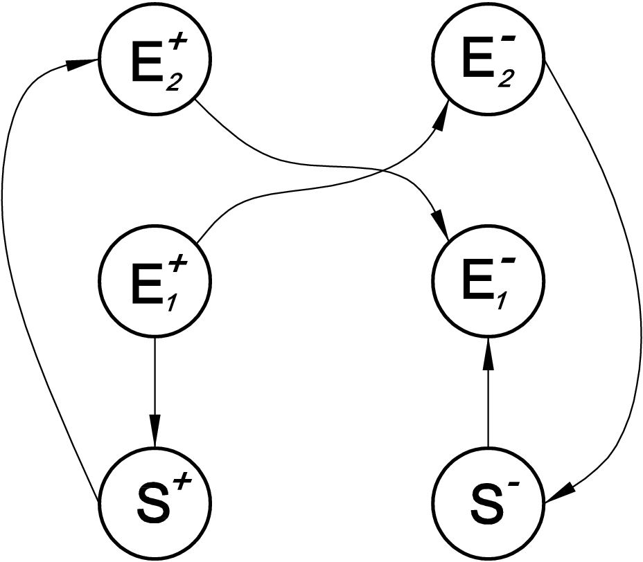
For , i.e. Side and Lateral cases, and for any to there exists a shortest path of type or of type . For , i.e. Frontal case, and for any to there exists a shortest path of type or of type .
Proof.
According to all propositions above several concatenations of extremal have been proved to be non optimal. Considering extremals as node and, possibly optimal, concatenations of extremal as edges of a graph, the sufficient optimal languages from in , for different values of and , are described in fig. 8. Indeed, it is straightforward to observe that the number of switches between extremals is finite and less or equal to 3, for any value of and . Hence, the thesis. ∎
|

We now study the length of extremal paths from to in the sufficient family above.
Without loss of generality, it is sufficient to study the length of extremal paths of type only from points on the semicircle of in the upper-half plane (denoted by ). Indeed, up to a rotation, optimal paths of type from the rest of can be easily obtained. Referring to fig. 9, let the switching points of the optimal path be denoted by , and or , and , respectively, depending on the angular values or . Moreover, in order to do the analysis, it is useful to parameterize the family by the angular value of the switching point along the arc between and or the angular value of the switching point along the extremal between and .
Theorem 5.
For any point , the length of a path of type is:
- •
for , i.e. from to (notice that the last arc has zero length):
- •
for , i.e. from to :
with and .
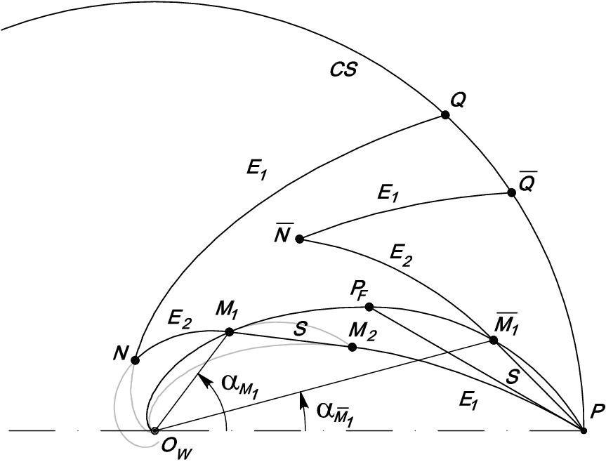
The analytical expression for the length is based on a direct computation. Having the path’s length as a function of two parameters or and , we are now in a position to minimize the length within the sufficient family.
Theorem 6.
Given a point ,
- •
for , optimal path is of type ;
- •
for with , optimal path is of type ;
- •
for the optimal path is through .
Moreover, for , any optimal path of type turns out to have the same length of optimal path . Hence, for also is optimal.
Previous results have been obtained computing first and second derivatives of and nonlinear minimization techniques.
We are now interested in determining the locus of switching points between extremals in optimal paths.
Proposition 4.
For with , the switching locus is the arc of between (included), where .
Proof.
From Theorem 6, the optimal path from to is of type . For the intersection between and is . ∎
Proposition 5.
For with , the loci of switching points and are the and .
Proof.
For with , considering the values of obtained in the computations of Theorem 6 we obtain . Furthermore, substituting those values in the equation of the intersection point between through and through we obtain . ∎
Finally, for with , the switching locus reduces to the origin since two extremal intersect only in the origin for .
5 Shortest paths from any point in the motion plane
The synthesis on induce a partition in regions of . Indeed, for any , there exists a point such that the optimal path from to goes through . The Bellmann’s optimality principle ensure the optimality of the sub–path from to . Based on this construction the partition of is reported in fig. 10.
| Region | Optimal Path |
|---|---|
| I | |
| II | |
| II′ | |
| III | |
| IV | |
| V | |
| V′ | |
| VI |

For points outside , function has been defined in 6 in order to transform paths starting from inside in paths starting from outside .
From other properties of , such as Proposition 1, we have also that an optimal path is mapped into an optimal path. Hence, the optimal synthesis from points outside can be easily obtained mapping through map all borders of regions inside .
Proposition 6.
Given a border and map transforms:
- 1.
into itself;
- 2.
in
- 3.
in
- 4.
in arcs of the same type ()
Proof.
The proof of this proposition can be found in [13]. ∎

6 Optimal synthesis for generic
We first obtain the synthesis of the Borderline Frontal case, i.e. , reported in fig. 12 from the one obtained in the previous section.

Notice that, of the Side case degenerates in a straight line through for . Indeed, referring to fig. 10, points and degenerate on . As a consequence, Region IV, IV and while coordinates and of points and can be obtained from values in 6 replacing .
In the Frontal case, becomes a spiral , straight lines from and split in straight line and a spiral arc generating the partition reported in fig. 13. In this case, and points and do not lay on but on a circle through with center , where . Notice that for , this circle coincide with and the synthesis proposed in [13] is obtained.

Referring again to fig. 10, in the Borderline Side case (, i.e. the SR border is aligned with the axle direction and ), degenerates in . Points and lays on with and . The obtained synthesis is reported in fig. 14.
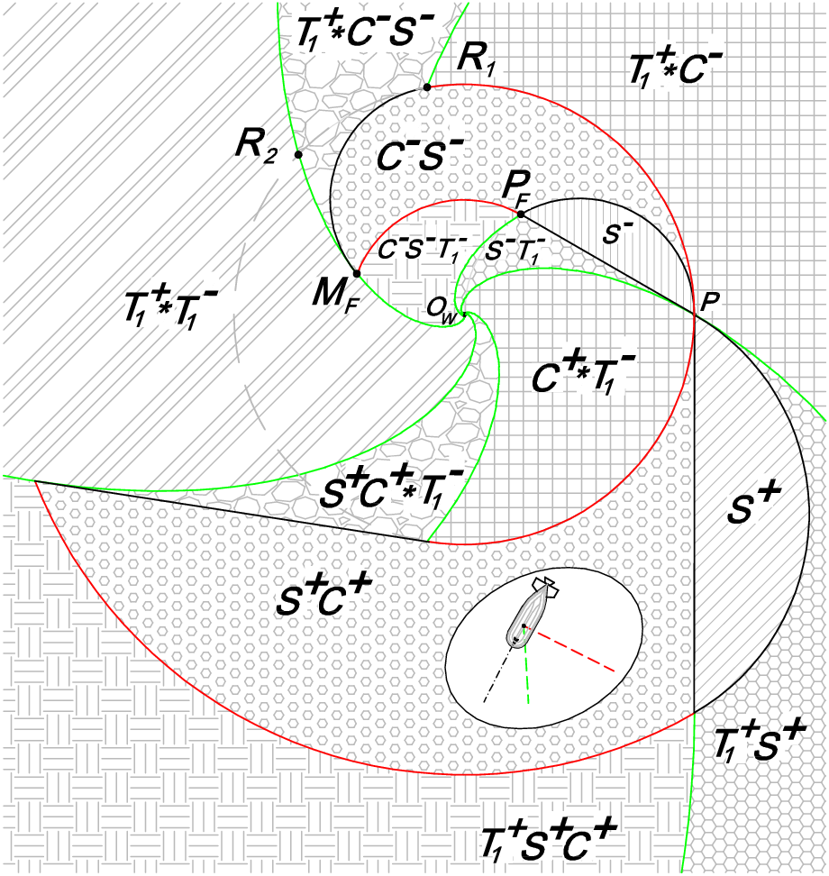
For the Lateral case becomes and the synthesis of the Lateral case, reported in fig. 15, can be obtained from the one in fig. 14.

The subdivision of the motion plane in case of can be easy obtained by using that one for considering optimal path followed in reverse order, i.e. forward arc in backward arc and viceversa. Finally, a symmetry w.r.t. axis of each subdivision of the motion plane for each allows to obtain the corresponding subdivision for .
7 Conclusions and future work
A complete characterization of shortest paths for unicycle nonholonomic mobile robots equipped with a limited range side sensor systems has been proposed. A finite sufficient family of optimal paths has been determined based on geometrical properties of the considered problem. Finally, a complete shortest path synthesis to reach a point keeping a feature in sight has been provided. A possible extension of this work is to consider a bounded 3D SR pointing to any direction with respect to the direction of motion. A more challenging extension would be considering a different minimization problem such as the minimum time.
References
- [1] D. Balkcom and M. Mason. Time-optimal trajectories for an omnidirectional vehicle. The International Journal of Robotics Research, 25(10):985–999, 2006.
- [2] S. Bhattacharya, R. Murrieta-Cid, and S. Hutchinson. Optimal paths for landmark–based navigation by differential–drive vehicles with field–of–view constraints. IEEE Transactions on Robotics, 23(1):47–59, February 2007.
- [3] A.E. Bryson and Y.C. Ho. Applied optimal control. Wiley New York, 1975.
- [4] X.N. Bui, P. Souères, J-D. Boissonnat, and J-P. Laumond. Shortest path synthesis for Dubins non–holonomic robots. In IEEE International Conference on Robotics and Automation, pages 2–7, 1994.
- [5] L. Cesari. Optimization-theory and applications: problems with ordinary differential equations. Springer-Verlag, New York, 1983.
- [6] H. Chitsaz, S. M. LaValle, D. J. Balkcom, and M.T. Mason. Minimum wheel-rotation for differential-drive mobile robots. The International Journal of Robotics Research, pages 66–80, 2009.
- [7] M. Chyba, N.E. Leonard, and E.D. Sontag. Optimality for underwater vehicle’s. In 40th IEEE Conference on Decision and Control, volume 5, pages 4204–4209, 2001.
- [8] N. Dias, C. Almeida, H. Ferreira, J. Almeida, A. Martins, A. Dias, and E. Silva. Manoeuvre based mission control system for autonomos surface vehicle. in Proceeedings of OCEANS ’09, May 2009.
- [9] L. E. Dubins. On curves of minimal length with a constraint on average curvature, and with prescribed initial and terminal positions and tangents. American Journal of Mathematics, pages 457–516, 1957.
- [10] F. Langner, C. Knauer, W. Jans, and A. Ebert. Side scan sonar image resolution and automatic object detection, classification and identification. in Proceeedings of OCEANS ’09, May 2009.
- [11] J. A. Reeds and L. A. Shepp. Optimal paths for a car that goes both forwards and backwards. Pacific Journal of Mathematics, pages 367–393, 1990.
- [12] P. Salaris, D. Fontanelli, L. Pallottino, and A. Bicchi. Optimal paths for mobile robots with limited field of view camera. In 48th IEEE Conference on Decision and Control, pages 8434–8439, Dec 2009.
- [13] P. Salaris, D. Fontanelli, L. Pallottino, and A. Bicchi. Shortest paths for a robot with nonholonomic and field-of-view constraints. IEEE Transactions on Robotics, 26(2):269–281, April 2010.
- [14] H. Souères and J. P. Laumond. Shortest paths synthesis for a car-like robot. IEEE Transaction on Automatic Control, pages 672–688, 1996.
- [15] H. Sussmann and G. Tang. Shortest paths for the reeds-shepp car: A worked out example of the use of geometric techniques in nonlinear optimal controlò. Technical report, Department of Mathematics, Rutgers University, 1991.
- [16] H. Wang, Y. Chan, and P. Souères. A geometric algorithm to compute time-optimal trajectories for a bidirectional steered robot. IEEE Transaction on Robotics, pages –, 2009.
.1 Proof of Theorem 1
Theorem 1.
Given two points and , with and , and an extremal path from to such that for each point of , , there exists an extremal path from to such that for each point of , and .
Proof.
Consider a point such that . Let and the sub–paths of from to and from to .
The sub–path , is rotated and scaled (contracted of factor ) such that is transformed in obtaining a path from to . Similarly, , can be rotated and scaled with the same scale factor but different rotation angle w.r.t. such that is transformed in , see fig. 3. After geometrical considerations, it is easy to notice that the obtained path starts in and ends in .
The obtained paths are a contraction of and respectively and hence shorter. Moreover, any point of or has hence is scaled in of or with .
Concluding, we have obtained a shorter path from to that evolves completely in the disk of radius . ∎
.2 Proof of Theorem 2
Theorem 2.
Any path consisting in a sequence of a backward extremal arc followed by a forward extremal arc is not optimal.
Proof.
Observe that the distance from is strictly increasing along backward extremal arcs (i.e. , , with ) and strictly decreasing along forward extremal arcs (i.e. , , with ). For continuity of paths, for any sequence of a backward extremal followed by a forward one, there exist points and that verify hypothesis of Theorem 1, hence it is not optimal.
Any sequence consisting in an extremal (or ) of length and an extremal (in any order and direction) is inscribed in two circumferences centered in . Hence, the shortest sequence is the one with along the circle of smaller radius necessarily preceded by a forward (or ) of same length .
Concluding, in an optimal path a forward arc cannot follow a backward arc. ∎