Finite temperature Casimir effect for graphene

As discussed in the introduction, the high temperature limit is the most intriguing regime in the Casimir physics. In this limit at distances $H\equiv 4\pi aT\gg 1$, the zero frequency Matsubara terms determine the free energy since other Matsubara terms are exponentially suppressed at these separations. As we show below, at zero frequency $r_{\rm TM}\sim 1$, $r_{\rm TE}\sim\alpha Nv_{F}^{2}|{\mathbf{p}}|$ for small values of the wave vector $|{\mathbf{p}}|$. Thus the coefficient $r_{\rm TM}$ acquires the ideal metal value, and this is the principal feature of graphene at high temperatures. At the same time, the TE mode free energy for graphene-metal is suppressed at separations $a\gtrsim 1/(4\pi T)$ by a factor $\alpha Nv_{F}^{2}/(aT)\ll 1$, and due to this suppression the difference in this regime in the results for the ideal metal and the Drude or the plasma models of a real metal is too small to be observed in possible experiments in graphene-metal system. For other distinctions of the graphene–metal high-temperature asymptotics see the next subsection.

As already mentioned the main contribution in the sum in (27) at high $aT$ is given by the zero frequency Matsubara term

where we also performed angular integration and re-scaled the momentum, $s=|{\mathbf{p}}|/T$ as compared with (27). Further expansion in powers of $aT$ is determined by the $s\to 0$ behavior of the integrand in (29). To obtain corresponding asymptotics we first note that the polarization tensor components at $\omega_{n}=0$ behave as

From this we readily deduce that

where we assumed that $m$ and $\mu$ are of the order of the temperature $T$, which can be relevant for some particular graphene samples and/or experimental setups. Note that all formulas in this section are also valid for $m,\mu\to 0$, since $s\to 0$ is essentially the same limit as $T\to\infty$.

As we can see, $r_{\rm\rm TE}$ remains small for the relevant values of momenta. Taking the leading term in the expansion of the logarithm in (29) and using (32) we obtain the leading TE contribution at large separations corresponding to the zero frequency term

For the TM mode one cannot use the expansion of $\ln(1-r_{\rm TM}e^{-2aTs})$ as it is divergent near $s=0$, see (33). Instead one has to use the representation

The integral of the first term can be taken explicitly leading to

which coincides exactly with the interaction of two real metals at high temperature described by the Drude model, or, equivalently, one half of interaction between two ideal metals at high temperature, ${\mathcal{F}}_{\rm id}$. For readability, in (36) we temporarily restored the physical units. In the rest of (35) one can use an expansion

As the main contribution to the asymptotics at $H\to\infty$ comes from vicinity of $s=0$ we can expand $r_{\rm TM}-1$ in a Taylor series around this point, to obtain in the highest order

where $C_{l}=\int_{0}^{\infty}s^{l+1}\left(\frac{e^{-s}}{1-e^{-s}}\right)^{l}ds$ and $r_{\rm\rm TM}^{(1)}\equiv\left(\frac{\partial}{\partial s}r_{\rm\rm TM}\right)_{s=0}$ which can be deduced from (33). In graphene, where $v_{F}^{2}/(\alpha N)\ll 1$, this correction is already small for considered $H=4\pi aT\gtrsim 1$, but in other Dirac systems with larger $v_{F}$, the transition of ${\mathcal{F}}_{0\rm TM}$ (35) to asymptotic (36) would occur only at much higher distances $aT\gg v_{F}^{2}/(\alpha N)$. We call attention of the reader that in any case this condition does not define the transition to the high-temperature regime of the whole free energy (27) which also includes the nonzero Matsubara terms. In the next subsection we investigate in detail their contribution and define through a scaling argument the transition condition for graphene-metal system as $aT\gg{\alpha\ln\alpha^{-1}}/(2\zeta(3))\simeq 0.015$.

Thus we can say, that from (34), (36) and (38), and considerations of the next subsection it follows that for separations $H\gg 0.19$ the main contribution to the interaction of a suspended graphene layer with ideal conductor comes from the TM mode leading contribution (36) and asymptotically constitutes just one half of the interaction between two ideal metals at large separations. This is induced by the specific dependence of the TE,M reflection coefficients on the momenta $s=|{\mathbf{p}}|/T$ for small $s$, see (32),(33). As mentioned earlier, such $r_{\rm TM,E}$ behavior also makes the predictions for large separations insensitive to the differences between Drude and plasma models of conductivity of a real metal in possible experiments. A numerical analysis shows that the difference between graphene-ideal metal and graphene-gold free energies becomes small already at $a\gtrsim 100$nm at $T=300$K (see Fig.2) and rapidly decreases with higher separations. Moreover, in this limit the interaction of two suspended graphene samples will acquire exactly the same asymptotical value.

As was shown in [9], in the zero-temperature limit the Casimir force between graphene and perfectly conducting metal is about $2.6\%$ of the force between two perfectly conducting metals. As we see, in the opposite limit, $H\gg 0.19$, the ratio of graphene - ideal metal free energy to the ideal metal - ideal metal free energy is strongly enhanced. Such an enhancement takes place due to the non-perturbative structure of the Lifshitz result in the limit $v_{F}=0$.

Given the specific values of $m$ and $\mu$, the Casimir interaction can be evaluated by making use of the Lifshitz formula, reflection coefficients and the polarization operator. As our numerical analysis shows, increasing the mass gap diminishes the Casimir interaction (see also a corresponding discussion in [9]), while inclusion of a nonzero chemical potential $\mu$ enhances the interaction. However, the difference in the values of the free energy for $m,\mu\sim 0.01$eV, which are reasonable bounds for these quantities in suspended graphene samples, and the $m=\mu=0$ case is less than one percent. Therefore in what follows we turn our attention to the important case $m=\mu=0$ and study it in detail.

It is often desirable to have an accurate analytical approximation of the exact result at different separations. We present such an expression for the sum of nonzero Matsubara terms in this section.

To obtain an appropriate analytical expression we first note that at separations $H\gg v_{F}$ one can put $v_{F}=0$ in any nonzero Matsubara term. It is possible due to the exponential factor in the Lifshitz formula which effectively restrains the integration over impulse to $ap_{\|}\lesssim 1$. In this case contribution of the type of $v_{F}^{2}(ap_{\|})^{2}$ can be neglected compared to $(ap_{0})^{2}=(2\pi naT)^{2}$ due to the smallness of the parameter $v_{F}$. However, our numerical analysis shows, that this approximation works at smaller distances as well, see below discussion around (46).

Secondly, in the finite temperature sum of nonzero Matsubara terms in the Lifshitz formula one can use the reflection coefficients taken at zero (!) temperature. The corrections due to finite temperature are suppressed for nonzero Matsubara terms, so we neglect them in the leading approximation. Contrary to this, in zero frequency Matsubara terms one has to take into account the whole structure of the finite temperature polarization operator entering $r_{TE,M}$.

Under two mentioned above approximations and the condition $m=\mu=0$ the reflection coefficients of a single graphene layer at zero temperature have the form:

Due to smallness of the reflection coefficients (both being of the order of $\alpha$) we can take just the first term in the expansion of the logarithm in the Lifshitz formula as another reasonable approximation for nonzero Matsubara terms. Note, however, that expansion of the reflection coefficients themselves (at least in TM mode) is not legitimate, as will become evident below.

The sum of nonzero Matsubara terms in this approximation in the TM case with $r^{(1)}_{\rm TM}=r_{\rm TM}^{T=0}$ (39) and $r^{(2)}_{\rm TM}=1$ equals to

here $s_{1}=\sqrt{\omega_{n}^{2}+p_{\|}^{2}}$ and $g\equiv 32Ta/(\alpha N)$, $E_{1}$ stands for the standard exponential integral function. It is convenient to reexpress the result (41) in an integral form. For this purpose one has to differentiate (41) over $H$, assuming $H$ as an independent parameter for the moment, calculate the sum over $n$ and then integrate back over $H$ (the integration constant is fixed as zero at $H\to\infty$). Thus one obtains

At large separations one can further approximate $8H+\pi\alpha Nt\approx 8H$ (i.e. expand in powers of $\alpha$) and get

The formula (43) provides an accurate description of (42) for $H\gtrsim 1$ where $\Delta\mathcal{F}_{\rm TM}$ constitutes less than $6$% of the whole answer. At $T=300$K this condition corresponds to distances greater than 600 nm. For smaller separations it is convenient to use (42) directly.

The TE part of the nonzero Matsubara terms of the Lifshitz formula with the coefficients $r^{(1)}_{TE}=r_{TE}^{T=0}$ from (40) and $r^{(2)}_{TE}=-1$ gives the following contribution in the leading order in $\alpha$

Thus, the complete result for the sum of nonzero Matsubara TM and TE terms in the approximation described above is given by (42) and (44)

Consequently, the leading $v_{F}=0$ contribution to the free energy is the sum of (36) and (45): ${\mathcal{F}}_{0\rm TM}^{(0)}+\Delta\mathcal{F}$. It can be used for the comparison of the theory and experiment almost at all separations. As our numerical analysis shows, a difference between the exact Lifshitz result $\mathcal{F}$ (27) (with $v_{F}=1/300$, $m=\mu=0$) and considered approximation ${\mathcal{F}}_{0\rm TM}^{(0)}+\Delta\mathcal{F}$ is less than $1\%$ for all separations between $1$ and $2000$ nm at the temperature $T=300$K, which approximately corresponds to $3.3\gtrsim H\gtrsim v_{F}/2=1/600$.

In our opinion, the distances corresponding to $H\gtrsim v_{F}$ (i.e. above $\sim 2$ nm for $T=300$K) are most relevant for a possible experiment, and the analytical expressions (42) and (44) are obtained to describe this particular regime. However, numerical studies reveal that $\Delta\mathcal{F}_{TM,E}$ are smooth in the vicinity of $H=0$ point, and collate with $T=0$ result obtained in [9]. Indeed, from (42) and (44) one gets in this limit

where the non analyticity in $\alpha$ comes from the TM mode, and explains the precautions we took avoiding to expand the reflection coefficient in (39). Since for $T\to 0$ the zero-frequency term $\mathcal{F}_{0}$ (29) vanishes, eq. (46) represents the free energy in the leading order in $\alpha$ in the approximation when $v_{F}=0$. The difference between (46) and the exact Lifshitz result at $T=0$ with $v_{F}=1/300$ is less than $1\%$. We also note that at $T=0$ the perturbative expansion in $\alpha$ is meaningful for $v_{F}\neq 0$ only, see [9].

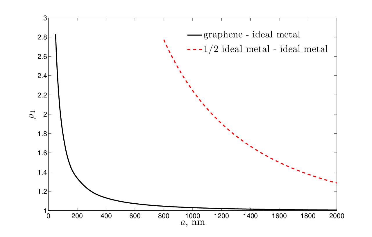
On Fig.1 we plot the ratio $\rho_{1}$ of the Lifshitz free energy $\mathcal{F}$ (27) divided by the high temperature asymptotics ${\mathcal{F}}_{0\rm TM}^{(0)}$ (36) at $T=300$K for two systems: graphene-ideal metal and ideal metal-ideal metal. From Fig.1 it is evident that the pace of approaching the asymptotic values by the free energy in the case of a graphene – ideal metal system is much higher than in the ideal metal–ideal metal one. It is explained by the particular behavior of the components of the polarization operator at nonzero frequencies

which induce additional $O(\alpha)$ suppression of the corresponding contributions to the free energy. Here, $c_{n}$, $\tilde{c}_{n}$ are factors of the order of unity. Because of this suppression the zero frequency TM Matsubara term dominates in the temperature dependence of the Lifshitz free energy for a graphene-metal system at much shorter separations than in the case of a metal-metal system.

It is instructive to define separate regimes on the basis of the scaling behavior of the free energy, rather than on validity of various approximations. As a function of distance, ${\mathcal{F}}\sim a^{-3+\delta}$, where $\delta=0$ at $T=0$ and $\delta=1$ at $T\to\infty$. The scaling parameter $\delta$ varies slowly, and can thus be defined through a logarithmic derivative

Since we are interested in rough estimates, it is enough to approximate $\mathcal{F}$ by a rational function

where $U$ can be defined by the $T=0$ value (46) and $V$ is calculated through the high temperature asymptotics, (36). Namely,

Consequently, (47) gives

We may consider the “zero temperature” regime as the one where $\delta$ is close to its $T=0$ value, let us say $\delta\lesssim 0.2$, giving $aT\lesssim 0.004$ or $a\lesssim 30{\rm nm}$ at $T=300K$. The high temperature regime, on the other hand, may be defined as $\delta\gtrsim 0.8$ corresponding to $aT\gtrsim 0.06$, or $a\gtrsim 460{\rm nm}$ at $T=300K$. Numerically, this bound is very close to one in the original condition, $H\gg 1$, which is universal for any Casimir system. However, in the graphene-metal interaction, as we already discussed, the high-temperature asymptotics is already saturated at $H\sim 1$, see Fig. 1. This can also be seen by considering an ‘intermediate’ scaling. At distances corresponding to $\delta=1/2$, where $H\approx 2\pi\alpha\ln\alpha^{-1}/\zeta(3)\approx 0.19$ is much smaller than unity, the high temperature asymptotic value already becomes larger than zero–$T$ contribution, i.e. $aV>U$, and thus this point can be considered (rather formally) as a crossover between zero and high-temperature regions.

It is interesting to note that the parameter $U$ which governs transitions between different regimes is defined by $\alpha$ and does not depend on $v_{F}$. One should not however overestimate this fact. All our expressions are valid for small $v_{F}$ only. In such a case the free energy behaves, very roughly, as a sum of the zero temperature contribution and the zeroth Matsubara term. Therefore, the crossover between different regimes is defined by the ratio of these two contributions.

On Fig.2 we plot the ratio $\rho_{2}$ of the free energy of a graphene-metal system to the ideal metal-ideal metal free energy at separations below $300$ nm. The temperature is chosen as $T=300$K, which means that $H=4\pi aT$ varies on Fig.2 from zero to 0.49. We used a plasma model for gold $\varepsilon(i\omega)=1+\omega_{p}^{2}/\omega^{2}$ with a plasma frequency $\omega_{p}=9.0$eV in numerical calculations of the free energy for gold semispace and a parallel graphene layer, gold reflection coefficients are standard Fresnel coefficients for TM, TE modes with a dielectric permittivity $\varepsilon(\omega)$, see [44]. The numerical result for the free energy of gold-graphene system divided by an ideal metal - ideal metal free energy is shown by the dashed blue curve on Fig.2. Note that the behavior of the gold-graphene free energy at short separations is one power of $a$ different from the graphene-ideal metal free energy. This is the usual change in power law when one approaches short separations and the transition from the retarded regime to a non-retarded one takes place at separations characterized by a material wavelength $\lambda_{p}=2\pi/\omega_{p}$. Thus, the result for a real metal interacting with graphene is essentially different from the ideal metal - graphene result at short separations only. The red curve which corresponds to the zero Matsubara term only is almost perfectly linear. This reflects the point that, as mentioned above, the expansion of $\mathcal{F}_{0\rm TM}$ around the high temperature asymptotics $\mathcal{F}_{0\rm TM}^{(0)}$ is governed by a small parameter $v_{F}^{2}/(\alpha N)$, while the term $\mathcal{F}_{0\rm TE}$ is suppressed by a factor $\alpha Nv_{F}^{2}$.