Transition magnetic moment of $\Lambda$ $\to$ $\Sigma^{0}$ in QCD sum rules

Frank X. Lee and Lai Wang Affiliation: Physics Department, The George Washington University, Washington, DC 20052, USA

Abstract

The $\Lambda$ $\to$ $\Sigma^{0}$ transition magnetic moment is computed in the QCD sum rules approach. Three independent tensor structures are derived in the external field method using generalized interpolating fields. They are analyzed together with the $\Lambda$ and $\Sigma^{0}$ mass sum rules using a Monte-Carlo-based analysis, with attention to OPE convergence, ground-state dominance, and the role of the transitions in the intermediate states. Relations between sum rules for magnetic moments of $\Lambda$ and $\Sigma^{0}$ and sum rules for transition magnetic moment of $\Lambda$ $\to$ $\Sigma^{0}$ are also examined. Our best prediction for the transition magnetic moment is $\mu_{\Sigma^{0}\Lambda}=1.60\pm 0.07\;\mu_{N}$ . A comparison is made with other calculations in the literature.

pacs

13.40.Em, 12.38.-t, 12.38.Lg, 11.55.Hx, 14.20.Gk, 14.20.Jn

I Introduction

Magnetic moment is an important property in the electromagnetic structure of baryons. In the case of octet baryons, various theoretical calculations have provided valuable insight into the underlying dynamics. The calculations benefited especially from the availability of precise experimental information on the magnetic moments. The $\Lambda$ $\to$ $\Sigma^{0}$ transition magnetic moment is considered a member in this octet family, so any theoretical approach for octet baryon magnetic moments should be able to provide an answer for this quantity. Relative to the attention paid to the individual members of the octet baryons, the $\Lambda$ $\to$ $\Sigma^{0}$ transition magnetic moment is less well-known.

The QCD sum rule method is a nonperturbative analytic formalism firmly entrenched in QCD with minimal modeling [1]. In this method, hadron phenomenology is linked with the interactions of quarks and gluon through a few parameters: the QCD vacuum condensates, giving an unique perspective on how the properties of hadrons arise from nonperturbative interactions in the QCD vacuum and how QCD works in this context. The method has been successfully applied to many aspects of strong-interaction physics. Calculations of the regular baryon magnetic moments have been carried out in QCD sum rules [2, 3, 4, 5, 6, 7, 8]. Limited study of the $\Lambda\to\Sigma^{0}$ transition magnetic moment was performed in the traditional QCD sum rule approach [9], and in the light-cone formulation of the approach [10].

In this work, we carry out a comprehensive, independent calculation of the transition magnetic moment of the $\Lambda$ $\to$ $\Sigma^{0}$ in the external field method in the traditional QCD sum rule approach. This would complete the picture in the electromagnetic structure of the octet baryons from the perspective of QCD sum rules. A number of improvements are made. First, we employ generalized interpolating fields which allow us to use the optimal mixing of interpolating fields to achieve the best match in a sum rule. Second, we derive a new, complete set of QCD sum rules at all three tensor structures and analyze all of them. The previous sum rules, which were mostly limited to one of the tensor structures, correspond to a special case of the mixing in our sum rules. Third, we perform a Monte-Carlo analysis which can give realistic error bars and which has become standard nowadays. Fourth, we analyze the three sum rules using the $\Lambda$ and $\Sigma^{0}$ mass sum rules derived from the same generalized interpolating fields. The performance of each of the sum rules is examined using the criteria of OPE convergence and ground-state dominance, along with the role of the transitions in intermediate states. Finally, we examine the relations between magnetic moment of $\Lambda$ and $\Sigma^{0}$ and transition magnetic moment of $\Lambda$ $\to$ $\Sigma^{0}$ , using the newly-derived QCD sum rules.

II Method

The starting point is the time-ordered correlation function in the QCD vacuum in the presence of a static background electromagnetic field $F_{\mu\nu}$ :

\Pi(p)=i\int d^{4}x\;e^{ip\cdot x}\langle 0\,|\,T\{\;\eta^{\Sigma^{0}}(x)\,\bar{\eta}^{\Lambda}(0)\;\}\,|\,0\rangle_{F}.

(1)

On the quark level, it describes a hadron as quarks and gluons interacting in the QCD vacuum. On the phenomenological level, it is saturated by a tower of hadronic intermediate states with the same quantum numbers. By matching the two descriptions, a connection can be established between hadronic properties and the underlying quark and gluon degrees of freedom governed by QCD. Here $\eta$ is the interpolating field that couples to the hadron under consideration. The subscript $F$ means that the correlation function is to be evaluated with an electromagnetic interaction term added to the QCD Lagrangian: ${\cal L}_{I}=-A_{\mu}J^{\mu},$ where $A_{\mu}$ is the external electromagnetic potential and $J^{\mu}=e_{q}\bar{q}\gamma^{\mu}q$ is the quark electromagnetic current.

Since the external field can be made arbitrarily small, one can expand the correlation function

\Pi(p)=\Pi^{(0)}(p)+\Pi^{(1)}(p)+\cdots,

(2)

where $\Pi^{(0)}(p)$ is the correlation function in the absence of the field, and gives rise to the mass sum rules of the baryons. The transition magnetic moment will be extracted from the QCD sum rules obtained from the linear response function $\Pi^{(1)}(p)$ .

The action of the external electromagnetic field is two-fold: it couples directly to the quarks in the baryon interpolating fields, and it also polarizes the QCD vacuum. The latter can be described by introducing new parameters called vacuum susceptibilities.

The interpolating field is constructed from quark fields with the quantum number of baryon under consideration and it is not unique. We consider a linear combination of the two standard local interpolating fields.

\begin{array}[]{l}\eta^{\Lambda}(uds)={-2\sqrt{\frac{1}{6}}}\epsilon^{abc}[2(u^{aT}C\gamma_{5}d^{b})s^{c}+(u^{aT}C\gamma_{5}s^{b})d^{c}\\ \;\;\;\;\;\;\;\;\;\;\;\;\;\;\;\;\;\;-(d^{aT}C\gamma_{5}s^{b})u^{c}\hskip 5.69054pt+\beta(2(u^{aT}Cd^{b})\gamma_{5}s^{c}\\ \;\;\;\;\;\;\;\;\;\;\;\;\;\;\;\;\;\;\;+(u^{aT}Cs^{b})\gamma_{5}d^{c}-(d^{aT}Cs^{b})\gamma_{5}u^{c})];\end{array}

(3)

\begin{array}[]{l}\eta^{\Sigma^{0}}(uds)=-\sqrt{2}\epsilon^{abc}[(u^{aT}C\gamma_{5}s^{b})d^{c}+(d^{aT}C\gamma_{5}s^{b})u^{c}\\ \;\;\;\;\;\;\;\;\;\;\;\;\;\;\;\;\;\;\;+\beta((u^{aT}Cs^{b})\gamma_{5}d^{c}+(d^{aT}Cs^{b})\gamma_{5}u^{c})].\end{array}

(4)

Here $C$ is the charge conjugation operator; the superscript $T$ means transpose; and $\epsilon_{abc}$ makes it color-singlet. The normalization factors are chosen so that correlation functions of these interpolating fields coincide with each other under SU(3)-flavor symmetry. The real parameter $\beta$ allows for the mixture of the two independent currents. The choice advocated by Ioffe [2] and often used in QCD sum rules studies corresponds to $\beta=-1$ . We will take advantage of this freedom to achieve optimal matching in the sum rule analysis.

II.1 Phenomenological Representation

We start with the structure of the two-point correlation function in the presence of the electromagnetic vertex to first order

\Pi(p)=i\int{d^{4}x}e^{ipx}<0|\eta^{\Sigma^{0}}(x)[-i\int{d^{4}y}A_{\mu}(y)J^{\mu}(y)]\bar{\eta}^{\Lambda}(0)|0>_{F}.

(5)

Inserting two complete sets of physical intermediate states, we restrict our attention only to the positive energy ones and write

\begin{array}[]{l}\Pi(p)=\int{d^{4}x}d^{4}y\frac{{d^{4}k^{\prime}}}{{(2\pi)^{4}}}\frac{{d^{4}k}}{{(2\pi)^{4}}}\sum\limits_{N^{\prime}N}{\sum\limits_{s^{\prime}s}{\frac{{-i}}{{k^{\prime 2}-M_{N^{\prime}}^{2}-i\varepsilon}}}}\frac{{-i}}{{k^{2}-M_{N}^{2}-i\varepsilon}}\\ e^{ipx}A_{\mu}(y)<0|\eta^{\Sigma^{0}}(x)|N^{\prime}k^{\prime}s^{\prime}><N^{\prime}k^{\prime}s^{\prime}|J^{\mu}(y)|Nks><Nks|\bar{\eta}^{\Lambda}(0)|0>.\\ \end{array}

(6)

The matrix element of the electromagnetic current has the general form

\begin{array}[]{l}<k^{\prime}s^{\prime}|J^{\mu}(0)|ks>=\bar{u}(k^{\prime},s^{\prime})[F_{1}(Q^{2})[\gamma_{\mu}+i{\frac{m_{\Sigma^{0}}-m_{\Lambda}}{Q^{2}}}q^{\mu}]-F_{2}(Q^{2})\sigma^{\mu\nu}{\frac{q^{\nu}}{m_{\Sigma^{0}}+m_{\Lambda}}}]u(k,s),\end{array}

(7)

where $q=k^{\prime}-k$ is the momentum transfer and $Q^{2}=-q^{2}$ . In the following, we treat $\Lambda$ and $\Sigma^{0}$ mass as degenerate because their mass difference is small and set $\bar{m}=\frac{m_{\Lambda}+m_{\Sigma^{0}}}{2}$ to be the average mass of $\Lambda$ and $\Sigma^{0}$ . The Dirac form factors $F_{1}$ and $F_{2}$ are related to the Sachs form factors by

\begin{array}[]{l}G_{E}(Q^{2})=F_{1}(Q^{2})+\frac{Q^{2}}{(2\bar{m})^{2}}F_{2}(Q^{2})\\ G_{M}(Q^{2})=F_{1}(Q^{2})+F_{2}(Q^{2}).\end{array}

(8)

At $Q^{2}=0$ , $F_{1}(0)=1$ , $F_{2}(0)=\mu_{\Sigma^{0}\Lambda}^{a}$ which is the anomalous transition magnetic moment, and $G_{M}(0)=F_{1}(0)+F_{2}(0)=\mu_{\Sigma^{0}\Lambda}$ which is the transition magnetic moment. Note that we consider here the transition $\Lambda\rightarrow\Sigma^{0}$ . The moment for the reverse transition is related by a minus sign: $\mu_{\Lambda\Sigma^{0}}=-\mu_{\Sigma^{0}\Lambda}$ .

Writing out explicitly only the contribution of the ground-state nucleon and denoting the excited state contribution by ESC, we arrive at

\begin{array}[]{l}\Pi(p)=\frac{{i}}{2}\lambda_{\Lambda}\lambda_{\Sigma^{0}}F_{\mu\nu}[p^{2}-\bar{m}^{2}-i\varepsilon]^{-2}(\hat{p}+\bar{m})\{\frac{{i(\mu_{\Sigma\Lambda}-1)}}{{2\bar{m}}}\sigma^{\mu\nu}(\hat{p}+\bar{m})+i\sigma^{\mu\nu}\\ -(p^{\mu}\gamma^{\nu}-p^{\nu}\gamma^{\mu})(\hat{p}+\bar{m})[p^{2}-\bar{m}^{2}-i\varepsilon]^{-1}\}+ESC,\end{array}

(9)

where $\lambda_{\Lambda}$ and $\lambda_{\Sigma^{0}}$ are phenomenological parameters that measure the overlap of the interpolating fields with the ground state. Examination of its tensor structure using Mathematica reveals that its has 3 independent combinations, which we name with the following short-hand notation:

\mbox{WE}_{1}=F^{\mu\nu}(\hat{p}\sigma_{\mu\nu}+\sigma_{\mu\nu}\hat{p}),\;\;\mbox{WO}_{1}=F^{\mu\nu}\sigma_{\mu\nu},\;\;\mbox{WO}_{2}=F^{\mu\nu}i(p_{\mu}\gamma_{\nu}-p_{\nu}\gamma._{\mu})\hat{p}.

(10)

They are the same as those for the magnetic moment of octet baryons [8]. Upon Borel transform the ground state takes the form

\hat{B}[\Pi(p)]=-\frac{\lambda_{\Lambda}\lambda_{\Sigma^{0}}}{{4M^{2}}}e^{-\bar{m}^{2}/M^{2}}\{\frac{1}{{\bar{m}}}(2\bar{m}^{2}\mu_{\Sigma^{0}\Lambda}-M^{2}(\mu_{\Sigma^{0}\Lambda}-1))[WO_{1}]+\mu_{\Sigma^{0}\Lambda}[WE_{1}]+\frac{{2(\mu_{\Sigma^{0}\Lambda}-1)}}{{\bar{m}}}[WO_{2}]\},

(11)

where $M$ is the Borel mass.

Here we must treat the excited states with care. For a generic invariant function, the pole structure in momentum space can be written as

\begin{array}[]{l}\frac{C_{N\leftrightarrow N}^{2}}{(p^{2}-\bar{m}^{2})^{2}}+\sum\limits_{N^{*}}{\frac{{C_{N\leftrightarrow N^{*}}^{2}}}{{(p^{2}-\bar{m}^{2})(p^{2}-\bar{m^{*}}^{2})}}}+\sum\limits_{N^{*}}{\frac{{C_{N^{*}\leftrightarrow N^{*}}^{2}}}{{(p^{2}-\bar{m^{*}}^{2})^{2}}}},\end{array}

(12)

where $C_{N\leftrightarrow N}$ , $C_{N\leftrightarrow N^{*}}$ and $C_{N^{*}\leftrightarrow N^{*}}$ are constants. The first term is the ground state pole which contains the desired transition magnetic moment $\mu_{\Sigma^{0}\Lambda}$ . The second term represents the non-diagonal transitions between the ground state and the excited states caused by the external field. The third term is pure excited state contributions. Upon Borel transform, it takes the form

\begin{array}[]{l}\frac{\lambda_{\Lambda}\lambda_{\Sigma^{0}}\mu_{\Sigma^{0}\Lambda}}{M^{2}}e^{-\bar{m}^{2}/M^{2}}+e^{-\bar{m}^{2}/M^{2}}\left[\sum\limits_{N^{*}}\frac{C_{N\leftrightarrow N^{*}}^{2}}{\bar{m^{*}}^{2}-\bar{m}^{2}}\left(1-e^{-\left(\bar{m^{*}}^{2}-\bar{m}^{2}\right)/M^{2}}\right)\right]+\sum\limits_{N^{*}}\frac{C_{N^{*}\leftrightarrow N^{*}}^{2}}{M^{2}}e^{-\bar{m^{*}}^{2}/M^{2}}.\end{array}

(13)

The important point is that the transitions give rise to a contribution that is not exponentially suppressed relative to the ground state. This is a general feature of the external-field technique. The strength of such transitions at each structure is a priori unknown and is an additional source of contamination in the determination of the transition magnetic moment $\mu_{\Sigma^{0}\Lambda}$ . The standard treatment of the transitions is to approximate the quantity in the square brackets by a constant, which is to be extracted from the sum rule along with the ground state property of interest. Inclusion of such contributions is necessary for the correct extraction of the magnetic moments. The pure excited state contributions are exponentially suppressed relative to the ground state and can be modeled in the usual way by introducing a continuum model and threshold parameter.

II.2 Calculation of the QCD Side

On the quark level, by contracting out the quark pairs in Eq. (1) using the interpolating fields in Eq. (3) and Eq. (4), we obtain the following master formula in terms of quark propagators,

	$\displaystyle\langle\Omega\,\|\,T\{\;\eta^{\Sigma^{0}}(x)\,\bar{\eta}^{\Lambda}(0)\;\}\,\|\,\Omega\rangle=-2\epsilon^{abc}\epsilon^{a^{\prime}b^{\prime}c^{\prime}}\{\;$
	$\displaystyle-S_{u}^{{aa}^{\prime}}\gamma_{5}CS_{s}^{{bb}^{\prime^{T}}}C\gamma_{5}S_{d}^{{cc}^{\prime}}+2S_{s}^{{aa}^{\prime}}\gamma_{5}CS_{u}^{{bb}^{\prime^{T}}}C\gamma_{5}S_{d}^{{cc}^{\prime}}-2S_{s}^{{aa}^{\prime}}\gamma_{5}CS_{d}^{{bb}^{\prime^{T}}}C\gamma_{5}S_{u}^{{cc}^{\prime}}$
	$\displaystyle+S_{d}^{{aa}^{\prime}}\gamma_{5}CS_{s}^{{bb}^{\prime^{T}}}C\gamma_{5}S_{u}^{{cc}^{\prime}}+S_{d}^{{aa}^{\prime}}{Tr}[\gamma_{5}CS_{s}^{{bb}^{\prime^{T}}}C\gamma_{5}S_{u}^{{cc}^{\prime}}]-S_{u}^{{aa}^{\prime}}{Tr}[\gamma_{5}CS_{s}^{{bb}^{\prime^{T}}}C\gamma_{5}S_{d}^{{cc}^{\prime}}]$
	$\displaystyle-\beta\gamma_{5}S_{u}^{{aa}^{\prime}}\gamma_{5}CS_{s}^{{bb}^{\prime^{T}}}CS_{d}^{{cc}^{\prime}}-\beta S_{u}^{{aa}^{\prime}}CS_{s}^{{bb}^{\prime^{T}}}C\gamma_{5}S_{d}^{{cc}^{\prime}}\gamma_{5}+2\beta\gamma_{5}S_{s}^{{aa}^{\prime}}\gamma_{5}CS_{u}^{{bb}^{\prime^{T}}}CS_{d}^{{cc}^{\prime}}$
	$\displaystyle+2\beta S_{s}^{{aa}^{\prime}}CS_{u}^{{bb}^{\prime^{T}}}C\gamma_{5}S_{d}^{{cc}^{\prime}}\gamma_{5}-2\beta\gamma_{5}S_{s}^{{aa}^{\prime}}\gamma_{5}CS_{d}^{{bb}^{\prime^{T}}}CS_{u}^{{cc}^{\prime}}-2\beta S_{s}^{{aa}^{\prime}}CS_{d}^{{bb}^{\prime^{T}}}C\gamma_{5}S_{u}^{{cc}^{\prime}}\gamma_{5}$
	$\displaystyle-\beta^{2}\gamma_{5}S_{u}^{{aa}^{\prime}}CS_{s}^{{bb}^{\prime^{T}}}CS_{d}^{{cc}^{\prime}}\gamma_{5}+2\beta^{2}\gamma_{5}S_{s}^{{aa}^{\prime}}CS_{u}^{{bb}^{\prime^{T}}}CS_{d}^{{cc}^{\prime}}\gamma_{5}-2\beta^{2}\gamma_{5}S_{s}^{{aa}^{\prime}}CS_{d}^{{bb}^{\prime^{T}}}CS_{u}^{{cc}^{\prime}}\gamma_{5}$
	$\displaystyle+\beta\gamma_{5}S_{d}^{{aa}^{\prime}}\gamma_{5}CS_{s}^{{bb}^{\prime^{T}}}CS_{u}^{{cc}^{\prime}}+\beta S_{d}^{{aa}^{\prime}}CS_{s}^{{bb}^{\prime^{T}}}C\gamma_{5}S_{u}^{{cc}^{\prime}}\gamma_{5}+\beta\gamma_{5}S_{d}^{{aa}^{\prime}}{Tr}[\gamma_{5}CS_{s}^{{bb}^{\prime^{T}}}CS_{u}^{{cc}^{\prime}}]$
	$\displaystyle+\beta S_{d}^{{aa}^{\prime}}\gamma_{5}{Tr}[CS_{s}^{{bb}^{\prime^{T}}}C\gamma_{5}S_{u}^{{cc}^{\prime}}]-\beta\gamma_{5}S_{u}^{{aa}^{\prime}}{Tr}[\gamma_{5}CS_{s}^{{bb}^{\prime^{T}}}CS_{d}^{{cc}^{\prime}}]-\beta S_{u}^{{aa}^{\prime}}\gamma_{5}{Tr}[CS_{s}^{{bb}^{\prime^{T}}}C\gamma_{5}S_{d}^{{cc}^{\prime}}]$
	$\displaystyle+\beta^{2}\gamma_{5}S_{d}^{{aa}^{\prime}}CS_{s}^{{bb}^{\prime^{T}}}CS_{u}^{{cc}^{\prime}}\gamma_{5}+\beta^{2}\gamma_{5}S_{d}^{{aa}^{\prime}}\gamma_{5}{Tr}[CS_{s}^{{bb}^{\prime^{T}}}CS_{u}^{{cc}^{\prime}}]-\beta^{2}\gamma_{5}S_{u}^{{aa}^{\prime}}\gamma_{5}{Tr}[CS_{s}^{{bb}^{\prime^{T}}}CS_{d}^{{cc}^{\prime}}],$		(14)

where $S^{ab}_{q}(x,0;F)\equiv\langle 0\,|\,T\{\;q^{a}(x)\,\bar{q}^{b}(0)\;\}\,|\,0\rangle_{F}$ is the fully interacting quark propagator in the presence of the electromagnetic field. The propagator can be derived from the operator product expansion (OPE). To first order in $F_{\mu\nu}$ and $m_{q}$ (assume $m_{u}=m_{d}=0,m_{s}\neq 0$ ), and up to $x^{4}$ , its expression can be found in Ref. [8].

II.3 The QCD Sum Rules

With the above elements in hand, it is straightforward to evaluate the correlation function by substituting the quark propagator into the master formula. We keep terms to first order in the external field and in the strange quark mass. Terms up to dimension 8 are considered. The algebra is very tedious. Each term in the master formula is a product of three copies of the quark propagator. There are hundreds of such terms summed over various color permutations. We used a Mathematica package MathQCDSR [11] that we developed to carry out the calculations. We confirmed that the QCD side has the same tensor structure as the phenomenological side.

Once we have the QCD side (LHS) and the phenomenological side (RHS), we can construct the sum rules by matching the two sides in the standard way. Since there are three independent tensor structures, three sum rules can be constructed.

At the structure $\mbox{WE}_{1}$ , the sum rule can be expressed in the following form

\begin{array}[]{l}{\rm{c}}_{\rm{1}}L^{-4/9}E_{2}(w)M^{4}+{\rm{c}}_{\rm{2}}m_{s}\chi aL^{-26/27}E_{1}(w)M^{2}+{\rm{c}}_{\rm{3}}\chi a^{2}L^{-4/27}E_{0}(w)+{\rm{c}}_{\rm{4}}bL^{-4/9}E_{0}(w)+({\rm{c}}_{\rm{5}}+{\rm{c}}_{\rm{6}})m_{s}aL^{-4/9}E_{0}(w)\\ +({\rm{c}}_{\rm{7}}+{\rm{c}}_{\rm{8}})a^{2}L^{4/9}\frac{1}{{M^{2}}}+{\rm{c}}_{\rm{9}}\chi m_{0}^{2}a^{2}L^{-18/27}\frac{1}{{M^{2}}}+{\rm{c}}_{\rm{10}}m_{s}m_{0}^{2}aL^{-26/27}\frac{1}{{M^{2}}}\\ =-{\tilde{\lambda}_{\Lambda}}{\tilde{\lambda}_{\Sigma^{0}}}[\frac{{\mu_{\Sigma^{0}\Lambda}}}{{M^{2}}}+A]e^{-\bar{m}^{2}/M^{2}},\end{array}

(15)

where the coefficients are given by:

\begin{array}[]{l}c_{1}=\frac{1}{4}(2(\beta^{2}+\beta+1)e_{u}-(\beta(\beta+2)+2)e_{d})\\ c_{2}=\frac{1}{4}\beta(3(\beta+1)e_{u}-(2\beta+3)e_{d})\\ c_{3}=-(\frac{1}{6})(\beta-1)(e_{d}-e_{u})(\beta+f_{s}+1)\\ c_{4}=\frac{1}{96}((e_{s}+5e_{u})\beta^{2}+4e_{u}\beta-(\beta+2)^{2}e_{d}+4e_{u})\\ c_{5}=\frac{1}{12}(e_{d}(-6f_{s}+\beta(\beta+3(\beta+4)f_{s}+10)-2)-2e_{u}(-3f_{s}+\beta\ (\beta+1)(6f_{s}+5)-1))\\ c_{6}=\frac{1}{12}(3e_{s}f_{s}\kappa\phi\beta^{2}+(\beta^{2}+\beta-2)e_{d}(2\kappa-\xi)+e_{u}\ (((\beta-2)\beta+4)\kappa+(\beta^{2}+\beta-2)\xi))\\ c_{7}=\frac{1}{18}(-e_{d}(\beta^{2}-2f_{s}\beta+5f_{s}-1)-(\beta-1)e_{u}(5f_{s}+\beta(3\ f_{s}-1)-1))\\ c_{8}=\frac{1}{36}(3e_{s}f_{s}\kappa\phi\beta^{2}+(\beta-1)e_{d}((5f_{s}+\beta(3f_{s}-1)-1)\ \kappa-(\beta+f_{s}+1)\xi)\\ \;\;\;\;\;\;\;\;+e_{u}((\beta^{2}-2f_{s}\beta+5f_{s}-1)\kappa+(\beta-1)\ (\beta+f_{s}+1)\xi))\\ c_{9}=\frac{1}{144}(e_{s}f_{s}\phi\beta^{2}+(\beta-1)e_{d}(5f_{s}+2\beta(f_{s}+2)+4)-e_{u}((f_{s}+4)\ \beta^{2}+3f_{s}\beta-5f_{s}-4))\\ c_{10}=\frac{1}{48}((5e_{u}(f_{s}+1)-2e_{s})\beta^{2}+6e_{u}(f_{s}+1)\beta-(\beta(\beta+6)-12)\ e_{d}(f_{s}+1)-12e_{u}(f_{s}+1)).\end{array}

(16)

In addition to the standard quark condensate, gluon condensate, and the mixed condensate which are rescaled as $a=-(2\pi)^{2}\,\langle\bar{u}u\rangle$ , $\hskip 5.69054ptb=\langle g^{2}_{c}\,G^{2}\rangle$ , $\langle\bar{u}g_{c}\sigma\cdot Gu\rangle=-m_{0}^{2}\,\langle\bar{u}u\rangle$ . Three vacuum susceptibilities caused by the external field are introduced: $\langle\bar{q}\sigma_{\mu\nu}q\rangle_{F}\equiv e_{q}\chi\langle\bar{q}q\rangle F_{\mu\nu}$ , $\langle\bar{q}g_{c}G_{\mu\nu}q\rangle_{F}\equiv e_{q}\kappa\langle\bar{q}q\rangle F_{\mu\nu}$ , $\langle\bar{q}g_{c}\epsilon_{\mu\nu\rho\lambda}G^{\rho\lambda}\gamma_{5}q\rangle_{F}\equiv ie_{q}\xi\langle\bar{q}q\rangle F_{\mu\nu}$ . Note that $\chi$ has the dimension of GeV^-2, while $\kappa$ and $\xi$ are dimensionless. The quark charge factors $e_{q}$ are given in units of electric charge: $e_{u}=2/3,\hskip 11.38109pte_{d}=-1/3,\hskip 11.38109pte_{s}=-1/3$ . Note that we choose to keep the quark charge factors explicit. The advantage is that it can facilitate the study of individual quark contribution to the transition magnetic moment. The parameters $f$ and $\phi$ account for the flavor-symmetry breaking of the strange quark in the condensates and susceptibilities: $f={\langle\bar{s}s\rangle\over\langle\bar{u}u\rangle}={\langle\bar{s}g_{c}\sigma\cdot Gs\rangle\over\langle\bar{u}g_{c}\sigma\cdot Gu\rangle},\hskip 11.38109pt\phi={\chi_{s}\over\chi}={\kappa_{s}\over\kappa}={\xi_{s}\over\xi}.$ The anomalous dimension corrections of the interpolating fields and the various operators are taken into account in the leading logarithmic approximation via the factor $L^{\gamma}=\left[{\alpha_{s}(\mu^{2})\over\alpha_{s}(M^{2})}\right]^{\gamma}=\left[{\ln(M^{2}/\Lambda_{QCD}^{2})\over\ln(\mu^{2}/\Lambda_{QCD}^{2})}\right]^{\gamma}$ where $\mu=500$ MeV is the renormalization scale and $\Lambda_{QCD}$ is the QCD scale parameter. As usual, the pure excited state contributions are modeled using terms on the OPE side surviving $M^{2}\rightarrow\infty$ under the assumption of duality, and are represented by the factors $E_{n}(w)=1-e^{-w^{2}/M^{2}}\sum_{n}{(w^{2}/M^{2})^{n}\over n!},$ where $w$ is an effective continuum threshold and it is in principle different for different sum rules and we will treat it as a free parameter in the analysis. Also, $\tilde{\lambda}$ is the rescaled current coupling ${\tilde{\lambda}\equiv(2\pi)^{2}\lambda}$ . The rescaling is done so there is no explicit factors of $\pi$ in the sum rules.

At the structure $\mbox{WO}_{1}$ , the sum rule can be expressed in the following form

\begin{array}[]{l}{\rm{c}}_{\rm{1}}m_{s}L^{-8/9}E_{2}(w)M^{4}+{\rm{c}}_{\rm{2}}\chi aL^{-16/27}E_{2}(w)M^{4}+({\rm{c}}_{\rm{3}}{\rm{+c}}_{\rm{4}})aE_{1}(w)M^{2}+{\rm{c}}_{\rm{5}}m_{s}\chi a^{2}L^{-16/27}E_{0}(w)\\ +{\rm{c}}_{\rm{6}}\chi abL^{-16/27}E_{0}(w)+({\rm{c}}_{\rm{7}}+{\rm{c}}_{\rm{8}})m_{s}a^{2}\frac{1}{{M^{2}}}+{\rm{c}}_{\rm{9}}ab\frac{1}{{M^{2}}}\\ =-{\tilde{\lambda}_{\Lambda}}{\tilde{\lambda}_{\Sigma^{0}}}\bar{m}\left[\frac{2\mu_{\Sigma^{0}\Lambda}}{M^{2}}+\frac{\mu_{\Sigma^{0}\Lambda}-1}{\bar{m}^{2}}+A\right]e^{-\bar{m}^{2}/M^{2}},\end{array}

(17)

where the coefficients are

\begin{array}[]{l}c_{1}=(\beta^{2}+\beta-2)(e_{d}-e_{u})\\ c_{2}=\frac{1}{6}((4\beta^{2}+\beta-5)e_{u}-(\beta^{2}+\beta-5)e_{d})\\ c_{3}=\frac{1}{6}(e_{d}(-3f_{s}+\beta(\beta(3f_{s}-2)+4)+1)-(\beta-1)e_{u}(-5\beta+3\ (\beta+1)f_{s}-1))\\ c_{4}=\frac{1}{24}((\beta-1)e_{u}(2(8\beta\kappa+\kappa)+(\beta+8)\xi)+e_{d}(2((7-5\beta)\ \beta+1)\kappa+(\beta(2\beta-7)+8)\xi))\\ c_{5}=\frac{1}{2}((\beta^{2}+\beta+1)e_{d}-(2\beta^{2}+\beta+1)e_{u})(f_{s}+1)\\ c_{6}=\frac{1}{144}((-2\beta^{2}+\beta+4)e_{d}+(\beta-1)(5\beta+4)e_{u})\\ c_{7}=\frac{1}{18}(e_{d}((7f_{s}+4)\beta^{2}+4f_{s}\beta+\beta-2f_{s}+4)-e_{u}((10f_{s}+7)\ \beta^{2}+4f_{s}\beta+\beta-2f_{s}+4))\\ c_{8}=\frac{1}{72}(e_{d}(f_{s}+\beta(\beta+4(\beta+1)f_{s}+4)+4)-e_{u}(f_{s}+\beta(7f_{s}\beta+4\ \beta+4f_{s}+4)+4))(2\kappa-\xi)\\ c_{9}=\frac{1}{288}((-2\beta^{2}+\beta+1)e_{d}-e_{u}-\beta(\beta(e_{s}-e_{u})+e_{u})).\end{array}

(18)

At the structure $\mbox{WO}_{2}$ , the sum rule can be expressed in the following form

\begin{array}[]{l}{\rm{c}}_{\rm{1}}m_{s}L^{-8/9}E_{1}(w)M^{2}+{\rm{c}}_{\rm{2}}\chi aL^{-16/27}E_{1}(w)M^{2}+({\rm{c}}_{\rm{3}}{\rm{+c}}_{\rm{4}})aE_{0}(w)+{\rm{c}}_{\rm{5}}m_{s}\chi a^{2}L^{-16/27}E_{0}(w)+{\rm{c}}_{\rm{6}}m_{0}^{2}aL^{-4/9}\frac{1}{{M^{2}}}\\ +c_{\rm{7}}\chi abL^{-16/27}\frac{1}{{M^{2}}}+({\rm{c}}_{\rm{8}}+{\rm{c}}_{\rm{9}})m_{s}a^{2}\frac{1}{{M^{4}}}{\rm{+c}}_{{\rm{10}}}ab\frac{1}{{M^{4}}}\\ =-\frac{{\tilde{\lambda}_{\Lambda}}{\tilde{\lambda}_{\Sigma^{0}}}}{\bar{m}}[\frac{{2(\mu_{\Sigma^{0}\Lambda}-1)}}{{M^{2}}}+A]e^{-\bar{m}^{2}/M^{2}},\end{array}

(19)

where the coefficients for $\Lambda\to\Sigma^{0}$ at $\mbox{WO}_{2}$ :

\begin{array}[]{l}c_{1}=\frac{1}{2}(\beta^{2}+\beta-2)(e_{d}-e_{u})\\ c_{2}=\frac{1}{6}(\beta-1)^{2}(e_{d}-e_{u})\\ c_{3}=\frac{1}{6}(e_{d}(\beta^{2}(3f_{s}+2)-3(f_{s}+1))-3(\beta^{2}-1)e_{u}(f_{s}+1))\\ c_{4}=\frac{1}{24}(3(\beta-1)e_{u}(\beta\xi-2\kappa)+e_{d}((3-2\beta)\beta\xi-2\ ((\beta-3)\beta+3)\kappa))\\ c_{5}=\frac{1}{6}(\beta-1)(e_{d}-e_{u})(-\beta+(\beta+3)f_{s}+3)\\ c_{6}=\frac{1}{24}((-e_{s}+e_{u}+4e_{u}f_{s})\beta^{2}+3e_{u}\beta-e_{u}(4f_{s}+5)-(\beta-1)e_{d}(2\ \beta+4(\beta+1)f_{s}+5))\\ c_{7}=\frac{1}{144}(\beta-1)^{2}(e_{d}-e_{u})\\ c_{8}=\frac{1}{18}(e_{u}((10f_{s}+7)\beta^{2}+4f_{s}\beta+\beta-2f_{s}+4)-e_{d}((7f_{s}+4)\ \beta^{2}+4f_{s}\beta+\beta-2f_{s}+4))\\ c_{9}=-(\frac{1}{72})(e_{d}(f_{s}+\beta(\beta+4(\beta+1)f_{s}+4)+4)-e_{u}(f_{s}+\beta(7f_{s}\beta+4\ \beta+4f_{s}+4)+4))(2\kappa-\xi)\\ c_{10}=\frac{1}{288}((\beta-1)(2\beta+1)e_{d}+e_{u}+\beta(\beta(e_{s}-e_{u})+e_{u})).\end{array}

(20)

Note that the sum rule from $\mbox{WE}_{1}$ involves only dimension-even condensates, so we call this sum rule chiral-even. The sum rule from both $\mbox{WO}_{1}$ and $\mbox{WO}_{2}$ involves only dimension-odd condensates, so we call them chiral-odd.

III Sum Rule Analysis

The sum rules for transition magnetic moment have the generic form of OPE - ESC = Pole + Transition, or

\Pi_{\Lambda\to\Sigma^{0}}(QCD,\beta,w,M^{2})={\tilde{\lambda}_{\Lambda}}{\tilde{\lambda}_{\Sigma^{0}}}\left({\mu_{\Sigma^{0}\Lambda}\over M^{2}}+A\right)e^{-\bar{m}^{2}/M^{2}},

(21)

where $QCD$ represents all the QCD input parameters. The mathematical task then boils down to the following: given the function $\Pi_{\Lambda\to\Sigma^{0}}$ with known QCD input parameters and the ability to vary $\beta$ , find the phenomenological parameters (mass $\bar{m}$ , transition magnetic moment $\mu_{\Sigma^{0}\Lambda}$ , transition strength $A$ , coupling strength ${\tilde{\lambda}_{\Lambda}}$ and ${\tilde{\lambda}_{\Sigma^{0}}}$ , and continuum threshold $w$ ) by matching the two sides over some region in the Borel mass $M$ . A $\chi^{2}$ minimization is best suited for this purpose. It turns out that there are too many fit parameters for this procedure to be successful in general. To alleviate the situation, we employ the corresponding mass sum rules for the particles [12, 8] which have a similar generic form of OPE - ESC = Pole, or

\Pi_{\Lambda}(QCD,\beta,w_{1},M^{2})=\tilde{\lambda}_{\Lambda}^{2}e^{-m_{\Lambda}^{2}/M^{2}},

(22)

\Pi_{\Sigma^{0}}(QCD,\beta,w_{2},M^{2})=\tilde{\lambda}_{\Sigma^{0}}^{2}e^{-m_{\Sigma^{2}}/M^{2}}.

(23)

They share some of the common parameters and factors with the transition sum rules. Note that the continuum thresholds may not be the same in different sum rules. By taking the following combination of the transition and mass sum rules,

\frac{\Pi_{\Lambda\to\Sigma^{0}}(QCD,\beta,w,M^{2})}{\sqrt{\Pi_{\Lambda}(QCD,\beta,w_{1},M^{2})\Pi_{\Sigma^{0}}(QCD,\beta,w_{2},M^{2})}}\\ =\frac{\mu_{\Sigma^{0}\Lambda}}{M^{2}}+A,

(24)

the couplings $\lambda$ and the exponential factors are canceled out. This is the form we are going to implement. By plotting the two sides as a function of $1/M^{2}$ , the slope will be the transition magnetic moment $\mu_{\Sigma^{0}\Lambda}$ and the intercept the transition strength $A$ . The linearity (or deviation from it) of the left-hand side gives an indication of OPE convergence and the role of excited states. The two sides are expected to match for a good sum rule. This way of matching the sum rules has two advantages. First, the slope, which is the transition magnetic moment of interest, is usually better determined than the intercept. Second, by allowing the possibility of different continuum thresholds, we ensure that both sum rules stay in their valid regimes.

We use the Monte-Carlo procedure [13, 8, 14] to carry out the search. In this method, the entire phase-space of the input QCD parameters is explored simultaneously, and is mapped into uncertainties in the phenomenological parameters. This leads to more realistic uncertainty estimates than traditional approaches.

The QCD input parameters are given as follows. The condensates are taken as $a=0.52\;GeV^{3}$ , $b=1.2\;GeV^{4}$ , $m^{2}_{0}=0.72\;GeV^{2}$ . For the factorization violation parameter, we use $\kappa_{v}=2.0$ . The QCD scale parameter is restricted to $\Lambda_{QCD}=0.15$ GeV. The vacuum susceptibilities have been estimated in studies of nucleon magnetic moments [2, 3, 15, 16], but the values vary depending on the method used. We use $\chi=-6.0\;GeV^{-2}$ and $\kappa=0.75$ , $\xi=-1.5.$ Note that $\chi$ is almost an order of magnitude larger than $\kappa$ and $\xi$ , and is the most important of the three. The strange quark parameters are placed at $m_{s}=0.15\;GeV$ , $f=0.83$ , $\phi=0.60$ [4, 15]. These input parameters are just central values. We will explore sensitivity to these parameters by assigning uncertainties to them in the Monte-Carlo analysis.

IV Results and Discussion

IV.1 Transition magnetic moments of $\Lambda\to\Sigma^{0}$

We analyzed all three sum rules. For each sum rule, we have in principle 6 parameters to determine: $\mu_{\Sigma^{0}\Lambda}$ , $A$ , $w$ , $w_{1}$ , $w_{2}$ , $\beta$ . But a search treating all six parameters as free does not work because there is not enough information in the OPE to resolve them. Here, we use the freedom to vary $\beta$ as an advantage to find the optimal match. Another parameter that can be used to our advantage is the continuum threshold $w_{1}$ for the mass sum rule. We fix it to the value that gives the best solution to the mass sum rule independently. For $\Lambda$ , $w_{1}=1.60$ GeV; for $\Sigma^{0}$ , $w_{2}=1.66$ GeV. This way the transition magnetic moment sum rule and the mass sum rule can stay in their respective valid Borel regimes. This leaves us with three parameters: $\mu_{\Sigma^{0}\Lambda}$ , $A$ , $w$ . Unfortunately, a three-parameter search is either unstable or returns values for $w$ smaller than the particle mass, an unphysical situation. Again we think this is a symptom of insufficient information in the OPE. So we are forced to fix the continuum threshold $w$ that corresponds to the best match for the central values of the QCD parameters.

The Borel window is determined by the following two criteria: OPE convergence and ground-state dominance. It is done iteratively. For each value of $\beta$ , we adjust the Borel window until the best solution is found. Based on the quality of the match, the broadness of the Borel window and its reach into the lower end (non-perturbative regime), the size of the continuum contribution, and the OPE convergence, we find that the chiral-odd sum rule at structure $\mbox{WO}_{2}$ is more reliable than the chiral-even sum rule at structure $\mbox{WE}_{1}$ and chiral-odd sum rule at structure $\mbox{WO}_{1}$ . The physical reason is that the contributions of positive- and negative-parity excited states partially cancel each other in the chiral-odd sum rules whereas they add up in the chiral-even sum rules. Since the $\mbox{WO}_{2}$ sum rule has power corrections up to $1/{M^{4}}$ while $\mbox{WO}_{1}$ sum rule power corrections only goes up to $1/{M^{2}}$ , the $\mbox{WO}_{2}$ sum rule is expected to be more reliable than the $\mbox{WO}_{1}$ sum rule. In the following, we present some detailed analysis of this sum rule in order to demonstrate how it produces the results.

Fig. 1 shows the matching of the two sides in Eq. (24). The left hand side is normalized OPE minus ESC contribution and the right hand side is pole plus transition contribution. According to the right-hand side of this equation, the plot should be linear as a function of $1/M^{2}$ , so we try to match the left hand side over a Borel window by a linear line. We can see that the two curves agree very well over the Borel window 1.2 to 1.7. Based on this match, the slope $1.60$ gives the transition magnetic moment $\mu_{\Sigma^{0}\Lambda}$ , and the intercept $0.17$ gives the transition contribution $A$ between intermediate states. This match was performed at $\beta=-0.2$ and $w=1.70$ GeV.

Refer to caption — Figure 1: The matching for the chiral-odd QCD sum rule at structure $\mbox{WO}_{2}$ in Eq. (19) as prescribed in Eq. (24). The error band is derived from about 2000 QCD parameter sets in the Monte Carlo analysis.

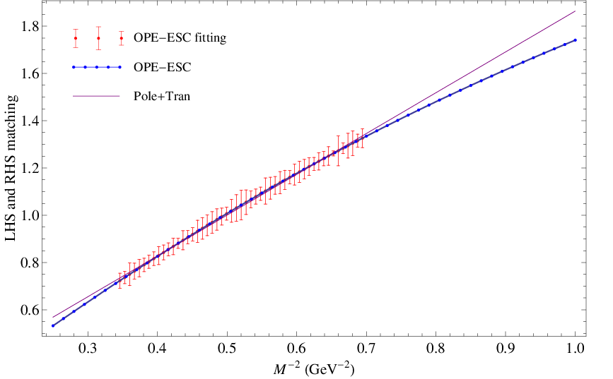
Figure 2 shows how the various terms in the OPE contribute to the determination of the transition magnetic moment. The $M^{2}$ term, which contains the contributions from the condensates $\chi a$ and strange quark mass $m_{s}$ , is the dominant term over the whole Borel region. The next leading contribution comes from $M^{0}$ term which involves condensates $a$ and $m_{s}\chi a^{2}$ , and is constant over the Borel region. The $M^{-2}$ term is from condensates $m_{0}^{2}a$ and $\chi ab$ , and is slightly negative over the region. The $M^{-4}$ term comes from condensates $m_{s}a^{2}$ and $ab$ , and is almost zero. These results confirm that the $WO_{2}$ sum rule has good OPE convergence and why it is the best sum rule out of the three structures. It also shows the importance of the vacuum susceptibility $\chi$ in the transition.

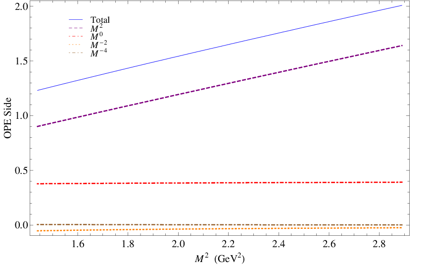
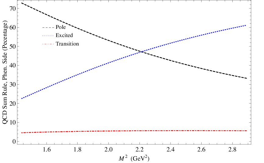
Figure 3 show various contributions in the phenomenological representation in $\mbox{WO}_{2}$ as a percentage of the total. We need to make sure that the ground-state pole is dominant. We can see that it is about 70% at the lower end of the Borel window. The transition contribution is small in this sum rule. It is consistently smaller than the excited-state contribution and has a weak dependence on the Borel mass. The excited-state contribution starts small, then grows with $M^{2}$ as expected from the continuum model. We cut off the Borel window when excited-state contribution goes too big, here it is around 60%.

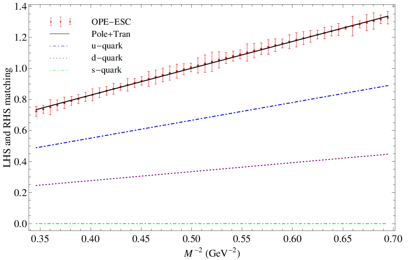
To gain a deeper understanding of the underlying quark-gluon dynamics, it is useful to consider the individual quark sector contributions to the transition magnetic moment. This can be done by dialing the corresponding charge factors $e_{q}$ in the sum rules which were explicitly kept for this purpose. Figure 4 shows a detailed matching of the two sides on Eq. (24) for the $\mbox{WO}_{2}$ sum rule, with individual contributions from u-, d- and s-quark. The four slopes are $0.80$ for total $\mu_{\Sigma^{0}\Lambda}$ and $0.53$ , $0.27$ and $0$ for u-, d- and s-quark. We see that the u-quark contributes about 67% to the total transition magnetic moment, d-quark about 33%, and s-quark almost zero. The slope for $\mbox{WO}_{2}$ comes from $\frac{2(\mu_{\Sigma^{0}\Lambda}-1)}{\bar{m}}$ , so it gives $\mu_{\Sigma^{0}\Lambda}=1.60\;\mu_{N}$ . To get the effective individual quark transition magnetic moment, we can use the percentage of individual contribution from the total transition magnetic moment. Then we have $\mu_{\Sigma^{0}\Lambda}^{u}=1.05\;\mu_{N}$ , $\mu_{\Sigma^{0}\Lambda}^{d}=0.53\;\mu_{N}$ and $\mu_{\Sigma^{0}\Lambda}^{s}\approx 0\;\mu_{N}$ . A closer examination reveals that the smallness of the s-quark contribution is due to an almost exact cancellation of the terms involving the s-quark, even though these terms are not small themselves.

Table 1: Results for

\Lambda\to\Sigma^{0}

from the three QCD sum rules. The ten columns correspond to, from left to right: structure,

\beta

value, Borel region in which the two sides of the QCD sum rule are matched, continuum threshold, percentage of excited state contribution on the phenomenological representation, transition strength, extracted transition magnetic moment in unit of nuclear magnetons, and effective u-, d- and s-quark transition magnetic moment. The errors are derived from 2000 samples in the Monte-Carlo analysis with 10% uncertainty on all QCD input parameters.

Structure	$\beta$	Region	$w$	ESC	A	$\mu_{\scriptscriptstyle\Sigma^{0}\Lambda}$	$\mu_{\Sigma^{0}\Lambda}^{u}$	$\mu_{\Sigma^{0}\Lambda}^{d}$	$\mu_{\Sigma^{0}\Lambda}^{s}$
		(GeV)	(GeV)	(%)	(GeV^-2)	$(\mu_{\scriptscriptstyle N})$	$(\mu_{\scriptscriptstyle N})$	$(\mu_{\scriptscriptstyle N})$	$(\mu_{\scriptscriptstyle N})$
WE1	-0.2	1.30 to 1.80	1.80	40-80	0.11(1)	1.57(8)	1.04(8)	0.53(3)	0(0)
WO1	-0.2	1.40 to 2.00	1.70	70-80	-0.46(9)	1.63(11)	1.08(11)	0.55(4)	0(0)
WO2	-0.2	1.20 to 1.70	1.70	20-60	0.17(4)	1.60(7)	1.05(10)	0.53(3)	0(0)

We analyzed sum rules at structures $\mbox{WE}_{1}$ and $\mbox{WO}_{1}$ in a similar fashion. The full results determined at the structures are given in Table 1. We see that our calculated transition magnetic moment is $1.60\pm 0.07\;\mu_{N}$ from the most reliable sum rule $\mbox{WO}_{2}$ . The other two sum rules also give close results around $1.60\;\mu_{N}$ . Our errors are derived from Monte-Carlo distributions which give more realistic estimation of the uncertainties. We find about 10% accuracy for the transition magnetic moment in our Monte-Carlo analysis, resulting from 10% uniform uncertainty in all the QCD input parameters. The uncertainties in the QCD parameters can be non-uniform. For example, we tried the uncertainty assignments (which are quite conservative) in Ref. [13], and found about 30% uncertainties in our output. One choice for $\beta$ here is $-0.2$ because it minimizes the perturbative term in the mass sum rule [17]. The excited state contribution at structure $\mbox{WO}_{2}$ is 20-60%, which gives reasonable pole dominance over the whole Borel region. On the other hand, the sum rules at $\mbox{WE}_{1}$ and $\mbox{WO}_{1}$ structures have larger contributions from the excited states over the Borel region. For this reason, we say the sum rules from $\mbox{WE}_{1}$ and $\mbox{WO}_{1}$ are less reliable. Another measure of reliability is the parameter $A$ , which is contamination from transitions between intermediate states. The A for the $\mbox{WO}_{1}$ sum rule is larger than those for the $\mbox{WE}_{1}$ and $\mbox{WO}_{2}$ sum rules, making it less reliable.

IV.2 Relations between QCD sum rules

It was pointed in Ref. [18] that it is possible to derive QCD rum rules for $\Lambda\to\Sigma^{0}$ from those for $\Sigma^{0}$ and $\Lambda$ . Here we would like to examine the issue using the generalized interpolating fields for $\Lambda$ and $\Sigma^{0}$ in Eq. (3) and Eq. (4).

The two-point correlation functions for magnetic moments of $\Lambda$ and $\Sigma^{0}$ are constructed from time-ordered product of operators $T\{\eta^{\Lambda}(x)\,\bar{\eta}^{\Lambda}(0)\}$ and $T\{\eta^{\Sigma^{0}}(x)\,\bar{\eta}^{\Sigma^{0}}(0)\}$ . The result is a master formula in terms of fully-interacting quark propagators in the QCD vacuum. Using the master formulas in Ref. [8], we have checked the following relations between the correlation functions

	$\displaystyle 2[\tilde{\Pi}^{\Sigma^{0}}_{d\leftrightarrow s}+\tilde{\Pi}^{\Sigma^{0}}_{u\leftrightarrow s}]-\Pi^{\Sigma^{0}}=3\Pi^{\Lambda},$		(25)
	$\displaystyle 2[\tilde{\Pi}^{\Lambda}_{d\leftrightarrow s}+\tilde{\Pi}^{\Lambda}_{u\leftrightarrow s}]-\Pi^{\Lambda}=3\Pi^{\Sigma^{0}}.$		(26)

Here $\tilde{\eta}^{\Lambda}_{d\leftrightarrow s}$ means the correlation function of $\Lambda$ but with d-quark and s-quark interchanged. The relations imply that one can obtain the QCD sum rules for $\Sigma^{0}$ by simple substitutions from the QCD sum rules for $\Lambda$ and vice versa. We confirmed that relations not only at the correlation function level, but at the level of the derived sum rules in [8]. It serves as an independent check of the QCD sum rules in Ref. [8].

The same argument can be extended to the $\Lambda\to\Sigma^{0}$ transition moment. There exist the following relations

	$\displaystyle\tilde{\Pi}^{\Sigma^{0}(u\leftrightarrow s)}-\tilde{\Pi}^{\Sigma^{0}(d\leftrightarrow s)}=\sqrt{3}\Pi^{\Sigma^{0}\Lambda},$		(27)
	$\displaystyle\tilde{\Pi}^{\Lambda(u\leftrightarrow s)}-\tilde{\Pi}^{\Lambda(d\leftrightarrow s)}=-\sqrt{3}\Pi^{\Sigma^{0}\Lambda}.$		(28)

This suggests that one can derive the QCD sum rules for the $\Lambda\to\Sigma^{0}$ transition magnetic moment by simple substitutions, starting from those for either $\Sigma^{0}$ or $\Lambda$ . In fact, we have calculated the QCD sum rules for $\Lambda\to\Sigma^{0}$ separately, and used the relations as independent checks of our calculations in this work and those in Ref. [8]. This was done both at the level of the master formula in Eq. (14) and at the level of the coefficients in the final QCD sum rules. The calculations has also served as a check of the Mathematica package [11].

IV.3 Comparison of results

Finally, we compare in Table 2 our result with experiment and other calculations. The list is only a representative sample, and necessarily incomplete. Unlike the other members of the octet, there was only one measurement for the $\Lambda\to\Sigma^{0}$ transition magnetic moment. It was done at Fermilab by utilizing the Primakoff effect [28]. Our result agrees with experiment. In the simple quark model, the transition moment can be related to the magnetic moment of $\Sigma^{+}$ and $\Sigma^{-}$ by $\mu_{\Sigma^{0}\Lambda}=(\mu_{\Sigma^{+}}-\mu_{\Sigma^{-}})\sqrt{3}/4$ . In terms of effective quark moments it is given by $\mu_{\Sigma^{0}\Lambda}=(\mu_{u}-\mu_{d})/\sqrt{3}$ . Using the values $\mu_{u}=1.852\;\mu_{N}$ and $\mu_{d}=-0.972\;\mu_{N}$ , it means that the u-quark contribution is about 67% of the total, the d-quark 33%, and the s-quark zero. Remarkably, our QCD sum rule results from the study of individual quark contributions are consistent with this composition. The lattice QCD result in Ref. [24] is quoted here by a scale factor of 1.18 as suggested in Ref. [29].

Table 2: Comparison of results for the

\Lambda\to\Sigma^{0}

transition magnetic moments in nuclear magnetons.

Method	$\mu_{\Sigma^{0}\Lambda}$
Experiment [19]	1.61(8)
QCD sum rule (this work)	1.60(7)
QCD sum rule [9]	1.5
Light-cone QCD sum rule [10]	1.60
Simple quark model [19, 20]	1.57(1)
Relativized quark model [21]	1.04
Quark model fits [22]	1.81
Chiral quark model [23]	1.71, 1.66, 1.61
Lattice QCD [24]	1.36
Chiral Perturbation Theory [25, 26]	1.42(1), 1.61(1)
Large-N ChPT [27]	1.576

V Conclusion

We have carried out a comprehensive study of the $\Lambda$ $\to$ $\Sigma^{0}$ transition magnetic moment using the method of QCD sum rules. We derived a complete set of QCD sum rules using generalized interpolating fields and analyzed them by a Monte-Carlo analysis. We determined the transition magnetic moment from the slope of straight lines. The linearity displayed from the OPE side matches almost perfectly with the phenomenological side in all cases. Out of the three independent structures, we find that the sum rule from the $\mbox{WO}_{2}$ structure is the most reliable based on OPE convergence and ground-state pole dominance. Our best prediction for the transition magnetic moment is $\mu_{\Sigma^{0}\Lambda}=1.60\pm 0.07\;\mu_{N}$ . More detailed results are listed in Table 1. The extracted transition magnetic moment is in good agreement experiment. Our Monte-Carlo analysis reveals that there is an uncertainty on the level of 10% in the transition magnetic moment if we assign 10% uncertainty in the QCD input parameters. We find that for all three sum rules, the u-quark contributes about $2/3$ of the total transition magnetic moment, d-quark about $1/3$ , while s-quark negligible due to an almost exact cancellation. This result agrees with the simple quark model. We verified certain relations that exist between the QCD sum rules and used them to check our calculations. Contrasted with results from a variety of other calculations, this study adds an unique perspective on the inner workings of the $\Lambda$ $\to$ $\Sigma^{0}$ transition magnetic moment in terms of the non-perturbative nature of the QCD vacuum.

Acknowledgements.

This work is supported in part by U.S. Department of Energy under grant DE-FG02-95ER-40907.

References

[1] M.A. Shifman, A.I. Vainshtein and Z.I. Zakharov, Nucl. Phys. B147, 385, 448 (1979).
[2] B.L. Ioffe and A.V. Smilga, Nucl. Phys. B232, 109 (1984).
[3] C.B. Chiu, J. Pasupathy, S.L. Wilson, Phys. Rev. D33 , 1961 (1986).
[4] J. Pasupathy, J.P. Singh, S.L. Wilson, and C.B. Chiu, Phys. Rev. D36 , 1442 (1986).
[5] S.L. Wilson, J. Pasupathy, C.B. Chiu, Phys. Rev. D36 , 1451 (1987).
[6] T.M. Aliev, A. Ozpineci, M. Savci, Phys. Rev. D66 , 016002 (2002).
[7] M. Sinha, A. Iqubal, M. Dey and J. Dey, Phys. Lett. B610, 283 (2005).
[8] L. Wang and F.X. Lee, Phys. Rev. D78, 013003 (2008).
[9] S.L. Zhu, W.Y.P. Hwang and Z.S. Yang, Phys. Rev. D57, 1527(1998).
[10] T. M. Aliev, A. Ozpineci, M. Savci, Phys. Lett. B516, 299 (2001).
[11] L. Wang and F.X. Lee, MathQCDSR: a Mathematica package for QCD sum rules calculations, submitted to Comp. Phys. Comm..
[12] F. X. Lee and X. Liu, Phys. Rev. D66, 014014 (2002).
[13] D. B. Leinweber, Ann. of Phys. (N.Y.) 254, 328 (1997).
[14] L. Wang and F.X. Lee, Phys. Rev. D80, 034003 (2009).
[15] F.X. Lee, Phys. Rev. D57, 1801 (1998).
[16] M. Sinha, A. Iqubal, M. Dey and J. Dey, Phys. Lett. B610, 283 (2005).
[17] S. Narison, Phys. Lett. B666, 455 (2008).
[18] A. Ozpineci, S.B. Yakovlev, V.S. Zamiralov, e-Print: hep-ph/0311271.
[19] Particle Data Group, J. Phys. G 38, 075021 (2010).
[20] J. Franklin, Phys. Rev. D29, 2648 (1984).
[21] M. Warnsa, W. Pfeila and H. Rollnika, Phys. Lett. B258, 431 (1991).
[22] A. Bohm , R.B. Teese, Phys. Rev. D26, 1103 (1982).
[23] H. Dahiya, M. Gupta, Phys. Rev. D67, 114015 (2003).
[24] D.B. Leinweber, Phys. Rev. D43, 1659 (1991).
[25] Ulf-G. Meißner, S. Steininger, Nucl.Phys. B499, 349-367 (1997).
[26] B. Kubis, Ulf G. Meissner, Eur. Phys. J. C18, 747 (2001).
[27] G. Ahuatzin, R. Flores-Mendieta, M.A. Hernandez-Ruiz, e-Print: arXiv:1011.5268 [hep-ph].
[28] P.C. Petersen et. al., Phys. Rev. Lett. 57, 949 (1986).
[29] D.B. Leinweber, Phys. Rev. D53, 5115 (1996).

Transition magnetic moment of Λ\Lambda →\to Σ0\Sigma^{0} in QCD sum rules