Exact Minimum-Repair-Bandwidth Cooperative Regenerating Codes for Distributed Storage Systems

Distributed storage systems such as Oceanstore [1] and Total Recall [2] provide reliable and scalable solutions to the increasing demand of data storage. They distribute data with redundancy to multiple storage nodes and the data can be retrieved even if some of nodes are not available. When erasure coding is used as a redundancy scheme in distributed storage, the task of repairing a node failure becomes non-trivial. A traditional way to repair a failed node is to download and reconstruct the whole data file first, and then regenerate the lost content (e.g., RAID-5, RAID-6). Since the size of the original data file may be huge, a lot of traffic is consumed for the purpose of repairing just one failed node.

In order to reduce the total traffic required for repairing, called repair-bandwidth, a new class of erasure codes, called regenerating codes [3], is presented and has a significantly lower traffic consumed in regenerating a failed node. The main idea of regenerating codes is to reduce repair-bandwidth from the survival nodes to a new node (called a newcomer), which regenerates the lost content in the failed node. Some constructions of minimum repair-bandwidth regenerating codes are given in [4, 5]. They are based on exact repair or called exact MBR codes, which means the lost content of the failed node are repaired exactly.

Most of the studies on regenerating codes in the literature are for the single-failure recovery or one-by-one repair. When the number of storage nodes becomes large, the multi-failure case is not infrequent, and we need to regenerate several failed nodes at the same time. In addition, in practical systems such as Total Recall, a recovery process is triggered only after the total number of failed nodes has reached a predefined threshold. These facts motivates the regeneration of multiple failed nodes jointly, instead of repairing in a one-by-one manner. A repair process in which the newcomers may exchange packets among themselves, called a cooperative repair or cooperative recovery, is first introduced in [6]. We will call the regenerating codes for multiple failures with cooperative repair cooperative regenerating codes. In [7], a special class of cooperative regenerating codes is proposed, in which the newcomers can select survival nodes for repairing flexibly. In [8], an explicit construction of cooperative regenerating code minimizing the storage in each node is given.

The tradeoff spectrum between repair-bandwidth and storage for cooperative regenerating codes is given in [8, 9]. Regenerating codes which attain one end of this spectrum, corresponding to the minimum storage, are considered in [6, 7]. In this paper, we focus on the other end of this spectrum. Codes which minimizes repair-bandwidth is called Minimal Repair-Bandwidth Cooperative Regenerating (MBCR) codes.

Main Results: After presenting a simple example and demonstrating the basic ideas in Section II, we derive in Section III a lower bound on the repair-bandwidth in cooperative recovery. An explicit construction of a family of exact MBCR codes matching this lower bound is given in Section IV.

In this section, we introduce some notations and illustrate the basic idea of cooperative repair.

Based on the system model introduced in [3] and [6], a file consisting of $B$ packets is encoded and distributed to $n$ nodes and a data collector can retrieve the file by downloading data from any $k$ of $n$ nodes. When $r$ nodes fails, $r$ newcomers are selected to repair the failed nodes. The repair process is divided into two phases. In the first phase, each of the $r$ newcomers connects to $d$ surviving nodes and downloads some packets. In the second phase, the newcomers exchange some packets among themselves. The objective is to minimize the total number of the packets transmitted (i.e., repair-bandwidth) in the two phases. Next we give an illustration of cooperative repair with parameters $n=4$ and $d=k=r=2$.

We initialize the distributed storage system by dividing a data file into eight data packets $A$, $B,\ldots,H$, and distribute them to four storage nodes. Each node stores five packets: four systematic and one parity-check (Fig. 1). The addition “+” is bit-wise exclusive-OR (XOR). The first node stores the first four packets $A$, $B$, $C$, $D$, skips the packet $E$, and stores the sum of the next two packets, $F+G$. The content of nodes 2, 3 and 4 can be obtained likewise by shifting the encoding pattern to the right respectively by 2, 4 and 6 packets. It is easy to verify that a data collector can rebuild the file from any two of four nodes in the illustrated code. For example, the data collector which connects to nodes 1 and 2 can reconstruct the eight data packets by downloading $A$, $B$, $C$ and $F+G$ from node 1, and $D$, $E$, $F$, and $H+A$ from node 2. Then it can solve for $G$ by subtracting $F$ from $F+G$, and $H$ by subtracting $A$ from $H+A$.

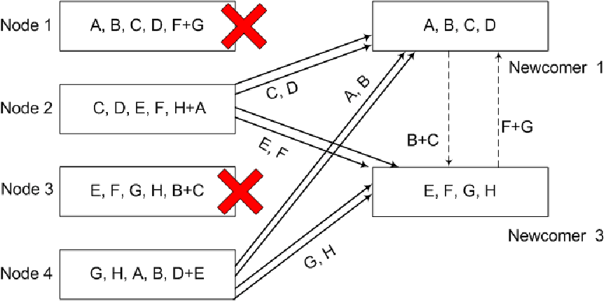
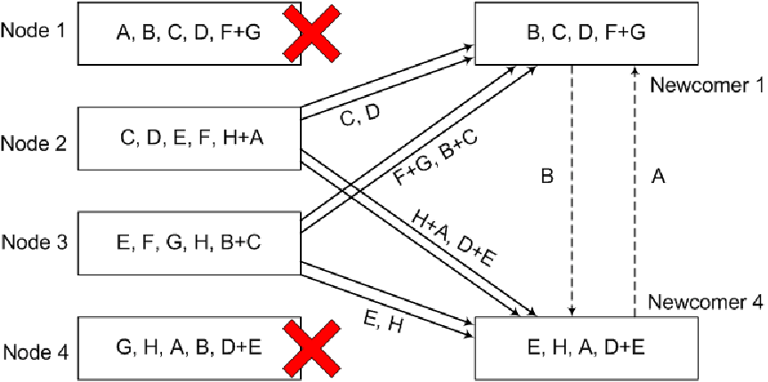
As for the repair process, the illustrated code costs ten packets per any two-failure recovery. Suppose that nodes 1 and 3 fail (see the first diagram in Fig. 1). Both newcomers 1 and 3 first download four packets from the survival nodes 2 and 4. Then newcomer 1 (resp. newcomer 3) computes the sum $B+C$ (resp. $F+G$) and sends it to newcomer 3 (resp. newcomer 1). Obviously, a total of ten packets, which are equal to the number of lines (including solid and dashed lines), are transmitted in the network. Similarly, should nodes 2 and 4 fail, the same repair-bandwidth is consumed for regeneration. Suppose that node 1 and 4 fail (see the second diagram in Fig. 1). Both newcomers 1 and 4 first download four packets from the survival nodes 2 and 3. Note that among the four downloaded packets, newcomer 1 (resp. newcomer 4) receives one encode packet $F+G$ (resp. $D+E$) from node 3 (resp. node 2). Then newcomer 1 solves for packet $B$ by subtracting $C$ from $B+C$, and transmits packet $B$ to newcomer 4. Also, newcomer 4 solves for packet $A$ and sends it to newcomer 1. Clearly, a total of ten packet transmissions are sufficient. Similarly, if any pair of two adjacent storage nodes fail, we can also repair them with ten packet transmissions, using the symmetry in the encoding for data distribution.

In this paper, we assume that the storage nodes are symmetrical; for the storage cost, each node stores $\alpha$ packets, and for the repair-bandwidth, each newcomer connects to $d$ existing nodes and downloads $\beta_{1}$ packets from each of them, and then sends $\beta_{2}$ packets to each of the $r-1$ other newcomers. In this paper, we only consider the case that $d\geq k$. The repair-bandwidth per newcomer, denoted by $\gamma$, is defined as the total number of the packets each newcomer receives, and thus is equal to

The aim of this section is to derive a lower bound on $\gamma$.

To formulate the problem, we draw an information flow graph as in [6]. Given parameters $n$, $k$, $d$, $r$, $\alpha$, $\beta_{1}$ and $\beta_{2}$, we construct an information flow graph $G=(\mathcal{V},\mathcal{E})$ as follows. The vertices are grouped into stages.

• •

  In stage $-1$, there is only one vertex $\mathsf{S}$, representing the source node which has the original file.

• •

  In stage 0, there are $n$ vertices $\mathsf{Out}_{1}$, $\mathsf{Out}_{2},\ldots,\mathsf{Out}_{n}$, each of them corresponds to an initial storage node. There is a directed edge with capacity $\alpha$ from $\mathsf{S}$ to each $\mathsf{Out}_{i}$.

• •

  For $t=1,2,3,\ldots$, suppose $r$ nodes fail in stage $t$. Let the indices of these $r$ storage nodes be $\mathcal{S}_{t}=\{j_{1}$, $j_{2},\ldots,j_{r}\}$. For each $i\in\mathcal{S}_{t}$, we put three vertices $\mathsf{In}_{i}$, $\mathsf{Mid}_{i}$ and $\mathsf{Out}_{i}$ in stage $t$. There are $d$ directed edges, with capacity $\beta_{1}$ from $d$ “out” vertices in previous stages to each $\mathsf{In}_{i}$. For each $i\in\mathcal{S}_{t}$, we put a directed edge from $\mathsf{In}_{i}$ to $\mathsf{Mid}_{i}$ with infinite capacity, and a directed edge from $\mathsf{Mid}_{i}$ to $\mathsf{Out}_{i}$ with capacity $\alpha$. For each pair of distinct indices $i,j\in\mathcal{S}_{t}$, we draw a directed edge from $\mathsf{In}_{i}$ to $\mathsf{Mid}_{j}$ with capacity $\beta_{2}$. The edges with capacity $\beta_{1}$ represent the data transferred from existing storage nodes to newcomers, and the edges with capacity $\beta_{2}$ represent the data exchanged among the newcomers.

• •

  To a data collector, who shows up after $s$ repair processes have taken place, we put a vertex $\mathsf{DC}$ in stage $s$ and connect it with $k$ “out” vertices with distinct indices in stage $s$ or earlier. The capacities of these $k$ edges are set to infinity.

An example of information flow graph for $n=4$ storage nodes and $d=r=k=2$ is shown in Fig. 2.

To derive a lower bound on $d\beta_{1}+(r-1)\beta_{2}$ for a file of fixed size $B$ is equivalent to derive a upper bound of $B$ for given capacities $\beta_{1}$ and $\beta_{2}$ in the information flow graph. So we can apply a celebrated max-flow theorem in [10], which says the size of the data file $B$ cannot be larger than the max-flow from $\mathsf{S}$ to any data collector ($\mathsf{DC}$). The max-flow is the maximal value of all feasible flows from $\mathsf{S}$ to $\mathsf{DC}$. Here, a flow from $\mathsf{S}$ to $\mathsf{DC}$, called an $(\mathsf{S},\mathsf{DC})$-flow, is a mapping $F$ from the set of edges to the set of non-negative real numbers, satisfying (i) for every edge $e$, $F(e)$ does not exceed the capacity of $e$, (ii) for any vertex $v$ except the source vertex $\mathsf{S}$ and the terminal vertex $\mathsf{DC}$, the sum of $F(e)$ over edges $e$ terminating at $v$ is equal to the sum of $F(e)$ over edges $e$ going out from $v$,

The value of an $(\mathsf{S},\mathsf{DC})$-flow $F$ is defined as

From the max-flow-min-cut theorem, we can upper bound the value of a flow by the capacity of a cut. For a given data collector $\mathsf{DC}$, an $(\mathsf{S},\mathsf{DC})$-cut is a partition $(\mathcal{U},\bar{\mathcal{U}})$ of the vertices in the information flow graph, such that $\mathsf{S}\in\mathcal{U}$ and $\mathsf{DC}\in\bar{\mathcal{U}}$, where $\bar{\mathcal{U}}$ stands for the complement of $\mathcal{U}$ in the vertex set $\mathcal{V}$. The capacity of an $(\mathsf{S},\mathsf{DC})$-cut is defined as the sum of capacities of the edges from vertices in $\mathcal{U}$ to vertices in $\bar{\mathcal{U}}$. Next, we will use the fact that the value of any $(\mathsf{S},\mathsf{DC})$-flow is less than or equal to the capacity of any $(\mathsf{S},\mathsf{DC})$-cut, together with the max-flow theorem in [10], to prove the following theorem.

Note: Theorem 2 is obtained independently in [9].

We can now show that the regenerating code discussed in Section II is optimal, in the sense that given the parameters $B$, $d$, $k$ and $r$, the repair-bandwidth matches the lower bound in Theorem 2. We have $B=8$ and $d=k=r=2$ in the example. From Theorem 2, the repair-bandwidth cannot be less than $8\frac{2\cdot 2+2-1}{2(2\cdot 2+2-2)}=5$. We have shown in Section II that the repair process requires exactly 5 packet transmissions per failed node, and therefore matches the optimal value.

For non-cooperative or one-by-one repair, it is proved in [3] that the minimum repair-bandwidth per failed node is $2dB/(k(2d+1-k))$, which turns out to be the same as the left hand side of (1) with $r$ set to 1. If we apply a non-cooperative regenerating code to a distributed storage system with parameters as in Section II, the minimum repair-bandwidth is $\frac{2\cdot 2\cdot 8}{2(2\cdot 2+1-2)}=5.333$. From this simple example, we can see that repair-bandwidth can be further reduced if some data exchange of data among the newcomers is allowed.

The lower bound of repair-bandwidth in Theorem 2 in fact holds via random linear coding with field size large enough. The tightness of the lower bound is established in [11], by showing the existence of MBCR codes which match the lower bound. Thus, the minimum repair-bandwidth for MBCR is indeed equal to $B(2d+r-1)/(k(2d+r-k))$.

We construct in this section a family of exact MBCR code with parameters $d=k$ and $n=d+r$. In fact, the illustrated code in Section II is a special case in this family.

The whole file is first divided into stripes. Each stripe consists of $B=k(2d+r-k)=kn$ data packets, considered as elements in $GF(q)$, where $q$ is a prime power. In each stripe let the $kn$ data packets be $x_{0}$, $x_{1},\ldots,x_{kn-1}$. We divide them into $n$ groups. The first group consists of $x_{0},x_{1},\ldots,x_{k-1}$, the second group consists of $x_{k},x_{k+1},\ldots,x_{2k-1}$, and so on. For notational convenience, we let $\mathbf{x}_{j}=[x_{(j-1)k}\ x_{(j-1)k+1}\ \ldots\ x_{(j-1)k+k-1}]$ be the vector of the data packets in the $j$th group ($1\leq j\leq n$).

For $i=1,2,\ldots,n$, we construct the content of node $i$ as follows. We first put the $k$ data packets in the $i$-th group $\mathbf{x}_{i}$ into node $i$ and then $n-1$ parity-check packets

into node $i$, where “$\cdot$” is the dot product of vectors and $\oplus$ is modulo-$n$ addition defined by

Here $\mathbf{v}_{j}$ ($j=1,2,\ldots,n-1$) are column vectors in a $k\times(n-1)$ generating matrix, $\mathbf{G}=[\mathbf{v}_{1}\ \mathbf{v}_{2}\ \ldots\ \mathbf{v}_{n-1}]$, of a maximal-distance separable (MDS) code over $GF(q)$ of length $n-1$ and dimension $k$. By the defining property of MDS code, any $k$ columns of $\mathbf{G}$ are linearly independent of $GF(q)$.

As for the file reconstruction processing, suppose without loss of generality that a data collector connects to nodes 1, $2,\ldots,k$. The systematic packets $x_{0},x_{1},\ldots,x_{k^{2}-1}$ in the first $k$ groups can be downloaded directly, because they are stored in node 1 to node $k$ uncoded. The $j$th group of data packets ($j>k$) (the components in vector $\mathbf{x}_{j}$) can be reconstructed from $\mathbf{x}_{j}\cdot\mathbf{v}_{j-1}$, $\mathbf{x}_{j}\cdot\mathbf{v}_{j-2},\ldots,\mathbf{x}_{j}\cdot\mathbf{v}_{j-k}$, by the MDS property. A data collector connecting to any other $k$ storage nodes can decode similarly.

As for the cooperative repair processing, suppose without loss of generality that nodes $k+1$ to $n$ fail at the same time. The repair process proceeds as follows.

Step 1:

For $i=1,2,\ldots,k$, node $i$ computes $\mathbf{x}_{i}\cdot\mathbf{v}_{n+i-j}$ and sends it to newcomer $j$, for $j=k+1,k+2,\ldots,n$.

Step 2:

For $j=k+1,k+2,\ldots,n$, newcomer $j$ downloads $k$ packets $\mathbf{x}_{j}\cdot\mathbf{v}_{j-1}$, $\mathbf{x}_{j}\cdot\mathbf{v}_{j-2},\ldots,\mathbf{x}_{j}\cdot\mathbf{v}_{j-k}$ from nodes 1 to $k$.

Step 3:

For $j=k+1,k+2,\ldots,n$, newcomer $j$ can solve for the systematic packets in $\mathbf{x}_{j}$. Then node $j$ sends $\mathbf{x}_{j}\cdot\mathbf{v}_{j+i}$ to node $n-i+1$, for $i=1,2,\ldots,n-j$, and sends $\mathbf{x}_{j}\cdot\mathbf{v}_{i}$ to node $j-i$, for $i=1,2,\ldots,j-k-1$.

In steps 1 and 2, a total of $2k(n-k)=2kr$ packets are transmitted. In step 3, each newcomer transmits $r-1$ packets. The total number of packets required in the whole repair process is $2kr+r(r-1)=r(2d+r-1)$. The number of packets per failed node is therefore $2d+r-1$. According to Theorem 2, the repair-bandwidth is no less than

Thus, this regenerating code is optimal.

Remark: If $n=q+2$ for some prime power $q$, we can use an extended Reed-Solomon (RS) code of length $q+1$ in the construction. The alphabet size could be as small as $n-2$. We refer the reader to [12] for the construction of extended RS code.

Example: An example for $n=5$, $d=k=3$ and $r=2$ is shown in Fig. 4. A stripe of file data is divided into 15 packets $x_{0}$, $x_{1},\ldots,x_{14}$. Let $q=2$ and $\mathbf{G}$ be the generating matrix

of a triply-extended Reed-Solomon code over $GF(2)$ [12]. The $i$th row of the array in Fig. 4 indicates the content of node $i$. For example, node 4 stores six systematic packets, $x_{9}$, $x_{10}$, $x_{11}$ in $\mathbf{x}_{4}$, $\mathbf{x}_{1}\cdot\mathbf{v}_{2}=x_{0}$, $\mathbf{x}_{2}\cdot\mathbf{v}_{3}=x_{4}$, $\mathbf{x}_{3}\cdot\mathbf{v}_{4}=x_{8}$, and one parity-check packet $\mathbf{x}_{5}\cdot\mathbf{v}_{1}=x_{12}+x_{13}+x_{14}$.

Suppose that nodes 4 and 5 fail. In the first step, node 1 sends $\mathbf{x}_{1}\cdot\mathbf{v}_{2}$ and $\mathbf{x}_{1}\cdot\mathbf{v}_{1}$ to newcomers 4 and 5 respectively. Similarly, node 2 sends $\mathbf{x}_{2}\cdot\mathbf{v}_{3}$ and $\mathbf{x}_{2}\cdot\mathbf{v}_{2}$, and node 3 sends $\mathbf{x}_{3}\cdot\mathbf{v}_{4}$ and $\mathbf{x}_{3}\cdot\mathbf{v}_{3}$. In the second step, node 1 transmits $\mathbf{x}_{4}\cdot\mathbf{v}_{3}$ and $\mathbf{x}_{5}\cdot\mathbf{v}_{4}$ to newcomers 4 and 5 respectively. Likewise, node 2 transmits $\mathbf{x}_{4}\cdot\mathbf{v}_{2}$ and $\mathbf{x}_{5}\cdot\mathbf{v}_{3}$, and node 3 transmits $\mathbf{x}_{4}\cdot\mathbf{v}_{1}$ and $\mathbf{x}_{5}\cdot\mathbf{v}_{2}$. In the third step, newcomer 4 reconstructs $\mathbf{x}_{4}$, and sends $\mathbf{x}_{4}\cdot\mathbf{v}_{4}$ to newcomer 5. Also, newcomer 5 reconstructs $\mathbf{x}_{5}$, and sends $\mathbf{x}_{5}\cdot\mathbf{v}_{1}$ to newcomer 4. Lastly, the lost packets in nodes 4 and 5 are regenerated in newcomer 4 and 5. The total number of packet transmissions in the whole repair process is equal to 14. The repair-bandwidth per failed node is 7. It matches the theoretic lower bound $15(2\cdot 3+2-1)/(3(2\cdot 3+2-3))=7$.

We give a construction of a family of exact and optimal MBCR codes for $d=k$ and $n=d+r$. The constructed regenerating code has the advantage of being a systematic code. For example, if we want to look at the content of one particular packet, we only need to contact the node which has a copy of this packet and download the packet directly. Another advantage of this construction is that the requirement of finite field size grows linearly as a function of the number of storage nodes.

References

- [1] J. Kubiatowicz et al., “OceanStore: an architecture for global-scale persistent storage,” in Proc. 9th Int. Conf. on Architectural Support for programming Languages and Operating Systems (ASPLOS), Cambridge, MA, Nov. 2000, pp. 190–201.
- [2] R. Bhagwan, K. Tati, Y. Cheng, S. Savage, and G. Voelker, “Total recall: system support for automated availability management,” in Proc. of the 1st Conf. on Networked Systems Design and Implementation, San Francisco, Mar. 2004.
- [3] A. G. Dimakis, P. B. Godfrey, Y. Wu, M. J. Wainwright, and K. Ramchandran, “Network coding for distributed storage systems,” IEEE Trans. Inf. Theory, vol. 56, no. 9, pp. 4539–4551, Sep. 2010.
- [4] K. V. Rashmi, N. B. Shah, P. V. Kumar, and K. Ramchandran, “Explicit construction of optimal exact regenerating codes for distributed storage,” in Allerton 47th Annual Conf. on Commun., Control, and Computing, Monticello, Oct. 2009, pp. 1243–1249.
- [5] C. Suh and K. Ramchandran, “Exact-repair MDS code construction using interference alignment,” IEEE Trans. Inf. Theory, vol. 57, no. 3, pp. 1425–1442, Mar. 2011.
- [6] Y. Hu, Y. Xu, X. Wang, C. Zhan, and P. Li, “Cooperative recovery of distributed storage systems from multiple losses with network coding,” IEEE J. on Selected Areas in Commun., vol. 28, no. 2, pp. 268–275, Feb. 2010.
- [7] X. Wang, Y. Xu, Y. Hu, and K. Ou, “MFR: Multi-loss flexible recovery in distributed storage systems,” in Proc. IEEE Int. Conf. on Comm. (ICC), Capetown, South Africa, May 2010.
- [8] K. W. Shum, “Cooperative regenerating codes for distributed storage systems,” in IEEE Int. Conf. Comm. (ICC), Kyoto, Jun. 2011.
- [9] A.-M. Kermarrec, N. Le Scouarnec, and G. Straub, “Repairing multiple failures with coordinated and adaptive regenerating codes,” Institut National de Recherche en Informatique et en automatique (INRIA), Rennes, Tech. Rep., Feb. 2011, arXiv:1102.0204.
- [10] R. Ahlswede, N. Cai, S.-Y. R. Li, and R. W. Yeung, “Network information flow,” IEEE Trans. Inf. Theory, vol. 46, pp. 1204–1216, 2000.
- [11] K. W. Shum and Y. Hu, “Existence of minimum-repair-bandwidth cooperative regenerating codes,” in Int. Symp. on Network Coding (Netcod), Beijing, Jul. 2011.
- [12] R. M. Roth, Introduction to Coding Theory. Cambrdige: Cambridge University Press, 2006.