Multiuser Diversity in Downlink Channels: When does the Feedback Cost Outweigh the Spectral Efficiency Gain?

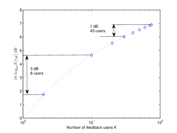
In this subsection, we quantify the benefit of multiuser diversity i.e., how the spectral efficiency increases w.r.t the number of feedback users when using dedicated feedback. The spectral efficiency is

where $\gamma_{df}=\max_{1\leq i\leq K}\gamma_{i}$ is the scheduled SNR, $\gamma_{i}=\lvert h_{i}\rvert^{2}$, $h_{i}\sim\mathcal{CN}\left(0,1\right)$ is the downlink channel of $i^{th}$ user and $P$ is the average SNR.

From [7], the spectral efficiency (1) has the following closed form expression

where $E_{1}(.)$ is the Exponential integral $\displaystyle{E_{1}(x)=\int^{\infty}_{x}\frac{e^{-t}}{t}~dt}$. Although (2) gives a closed form expression, it does not quantify how $C_{df}\left(K\right)$ increases with $K$. To quantify the growth rate of $C_{df}\left(K\right)$ with $K$, the following upper bound and lower bound on $C_{df}\left(K\right)$ are useful.

In Frequency Divison Duplexing (FDD) systems, the uplink and downlink have separate bandwidths. Fig.2.a shows the structure of the uplink and downlink bandwidths in a FDD system. The downlink bandwidth is used only for downlink data whereas the uplink bandwidth is used for SNR feedback (to aid downlink) and uplink data. Every coherence block, the uplink bandwidth is split into 2 pieces, the first one used for SNR feedback and the second one used for data transmission. At the begining of each uplink bandwidth, $K$ users feedback SNR to the BS. Let $\mathrm{W_{\mathrm{{fb}}}(K)}$ be the number of symbols used for SNR feedback on the uplink. $\mathrm{W_{\mathrm{{fb}}}(K)}$ will be defined separately for each of the 2 types of SNR feedback methods in the later sections. The remaining $\check{T}-\mathrm{W_{\mathrm{{fb}}}(K)}$ symbols are used for uplink data. The uplink rate is determined by the uplink data bandwidth and uplink spectral efficiency. The uplink data bandwidth $\mathrm{W_{\mathrm{{data}}}(K)}$, normalized to the total uplink bandwidth $\check{T}$, is

We model the uplink channel as an AWGN channel with SNR $P$, and hence the uplink spectral efficiency is

Therefore, the uplink rate is

Since the downlink bandwidth is only used for data, on downlink $\mathrm{W_{\mathrm{data}}}(K)=1$. The downlink spectral efficiency is

where $\gamma_{sch}$ is the scheduled SNR, expression for which depends on the type of SNR feedback method. Therefore, the downlink rate is

Increasing the number of feedback users increases the downlink rate but decreases the uplink data bandwidth and thus, decreases the uplink rate. ³³ 3 SNR feedback using downlink bandwidth can be used to increase the spectral efficiency on the uplink. This leads to a very similar tradeoff between uplink and downlink rates, and the basic insights found here apply to that scenario as well. Clearly there exists a tradeoff between the uplink and downlink rates. This tradeoff can be quantified by considering the maximization of the weighted sum of the uplink and downlink rates.

where $\lambda_{R}$ is the weight factor, specifying the preference of the downlink rate over the uplink rate. Thus, our fundamental objective is to determine the optimal number of feedback users as function of the system parameters blocklength, average SNR and weight factor.⁴⁴ 4 If the total number of users in the system is $K_{total}$, our objective is to find the number of feedback users $K$ from among $K_{total}$ which achieves an optimal balance between the uplink and downlink rates.

Time Divison Duplexing (TDD) systems differ from the FDD systems in that one common bandwidth is used for both the uplink and downlink. Fig.2.b shows the structure of the common bandwidth for both the uplink and downlink in a TDD system. Every coherence block, the bandwidth is split into 2 pieces, the first one used for SNR feedback on the uplink and the second one used for data transmission on the downlink.⁵⁵ 5 In TDD systems employing dedicated feedback, the users can alternatively send uplink pilots to allow the BS to estimate the per-user SNR. Although we don’t explicitly refer to this mode of operation in the paper, it is straightforward to see that it fits into our framework. For the sake of simplicity, it is assumed that there is no uplink data. It is explained later in section IV that even if the uplink data is present, it won’t change the cost-benefit tradeoff of multiuser diversity in a TDD system. At the begining of each bandwidth, users feedback SNR to the BS on the uplink using $\mathrm{W_{\mathrm{{fb}}}(K)}$ symbols. The number of data symbols on the downlink is $\check{T}-\mathrm{W_{\mathrm{{fb}}}(K)}$. The downlink rate is determined by the downlink data bandwidth and the spectral efficiency. It is given by

From (11), we see that the two terms which determine the downlink rate have a tradeoff with the number of feedback users, since the spectral efficiency increases and the data bandwidth decreases in $K$. Thus, our fundamental objective is to determine the optimal number of feedback users, in terms of maximizing the downlink rate, as function of the system parameters blocklength and average SNR.

In dedicated feedback, each user is allocated orthogonal feedback resources per coherence block i.e., a fixed number of symbols on the uplink for SNR feedback. Each user uses $L_{fb}$ bits for SNR feedback. The number of feedback symbols per user will be $\frac{L_{fb}}{\log_{2}\left(1+P\right)}$. So the feedback bandwidth in (5) is $W_{fb}(K)=\frac{KL_{fb}}{\log_{2}\left(1+P\right)}=O(K)$ and the uplink rate of a FDD system is

where $T=\frac{\check{T}}{L_{fb}}$ is the effective blocklength. The downlink rate of a FDD system is $R_{D}\left(K\right)=\mathbb{E}\left[\log_{2}\left(1+P\gamma_{df}\right)\right]$.⁶⁶ 6 We ignore the effect of $L_{fb}$ bit quantization of the SNR value at the user and assume that the feedback channel is error free. These simplifications simplify the analysis yet capturing the cost-benefit tradeoff of multiuser diversity which is primarily quantified in terms of the number of feedback users. These simplications are reasonable enough since $L_{fb}$ is large enough such that the high precision quantized SNR value very closely approximates the unquantized SNR value, the errors in the feedback channel can be made very small by using standard QAM methods [8]. The cost of an additional feedback user is $\frac{dR_{U}}{dK}=\frac{-1}{T}$ and it specifies the decrease in the uplink rate. The benefit of an additional feedback user is $\frac{dR_{D}}{dK}=O\left(\frac{1}{K\log K}\right)$ since $R_{D}\left(K\right)=O\left(\log\log K\right)$ from (4) and it specifies the marginal increase in the downlink rate. The tradeoff between the uplink and downlink rates is more clearly illustrated in Fig.3. From the figure, it is very clear that an optimized system should operate in region C which achieves a better tradeoff between the uplink and downlink rates than the regions A and B. The optimal operating point on the tradeoff curve can be quantified by solving the optimization problem in (10),

The objective function in (13) is concave and at the optimal operating point, the benefit of an additional feedback user on the downlink will equal the cost of an additional feedback user on the uplink i.e., $\frac{dR_{D}}{dK}=\frac{-1}{\lambda_{R}}\frac{dR_{U}}{dK}$. It is very difficult to obtain a closed form expression for $K^{df}_{op}$. In an effort to get an expression for $K^{df}_{op}$, we define a tight approximation to the downlink rate based on the upper and lower bounds in (3), $R_{D}\left(K\right)\approx\tilde{R}_{D}\left(K\right)=\log_{2}\left(1+P\log K\right)$ . The optimization problem is defined for the approximation

The solution to the above optimization problem is given in the following theorem.

SNR dependent feedback introduced in [3] has the basic idea that since only the good users (those with a large instantaneous SNR) will be scheduled, feedback bandwidth can be reduced significantly by asking only the good users to feedback SNR. Users with good SNR are differentiated from users with bad SNR by a SNR threshold $\gamma_{th}$. The SNR independent feedback method considered in the previous subsection wastes bandwidth since users with bad SNR also feedback SNR. Users compare their SNR $\gamma$ to a predetermined $\gamma_{th}$ and only if $\gamma\geq\gamma_{th}$, SNR is fedback on a random access channel. The choice of $\gamma_{th}$ determines how many users feedback SNR and thus the feedback bandwidth. The feedback random access channel can be implemented as a slotted ALOHA channel [2, 4] or CDMA channel [5].

We consider the slotted ALOHA like random access channel introduced in [4]. The random access channel has N slots as illustrated in Fig.2.c (in this paper, a slot refers to a fixed number of symbols grouped together). A user is eligible to feedback SNR only if $\gamma\geq\gamma_{th}=\log\left(\frac{K}{N}\right)$. An eligible user will select one of the N slots with probability $\frac{1}{N}$ to feedback its SNR and MS ID. Each user feeds back $L_{fb}$ bits of SNR value and $\log_{2}K$ bits of MS ID. The number of feedback symbols required for a user is $\frac{L_{fb}+\log_{2}K}{\log_{2}(1+P)}$. These many symbols are grouped into one feedback slot. A feedback attempt by a user is successful (hereafter referred to as user being captured) only if that user is the only one to attempt feedback in its selected slot, because a collision occurs when multiple users select the same slot. After $N$ slots of SNR feedback, the BS selects the user with the best downlink SNR from amongst the captured users. A more generalized SNR feedback algorithm is given in [2], although it is very complex.
The uplink data bandwidth is given by

The downlink spectral efficiency is

$\gamma_{sdf}=\max_{1\leq m\leq X}\gamma_{m\lvert\gamma_{th}}$ is the scheduled SNR, $\gamma_{m\lvert\gamma_{th}}$ is the SNR of the $m^{th}$ captured user and $X$ is the number of captured users. The sum rate is

An expression for $P\left(X\geq 1\right)$ is given in Appendix C. The weighted sum rate optimization is

Based on the expression for the sum rate (20) in Appendix C, it is easily seen that the optimization in (21) does not have a closed form solution and has to be solved numerically. Intuitively, the value of $K^{sdf}_{op}$ can be easily understood. The feedback bandwidth in SNR dependent feedback (20) is $O(\log K)$, unlike $O(K)$ in dedicated feedback, and this literally allows for all of the available multiuser diversity to be used i.e., all users in the system can participate in the feedback process. In Fig.4, $K^{sdf}_{op}$ is plotted against the blocklength at 10 and 0 dB. It is seen that all the 75 users in the system can participate in the feedback process.

Fig.6 plots the weighted sum rates of both the feedback methods against the number of feedback users. Fig.6 summarizes the key findings of this section i.e., for dedicated feedback, due to the significant feedback cost, the number of feedback users has to be very carefully selected, and for SNR dependent feedback, due to the relatively much smaller feedback cost, all the users in the system can participate in the feedback process.

The feedback process in a TDD system is the same as in a FDD system (section III-A) except that it consumes bandwidth common to both the uplink and downlink. The downlink rate of a TDD system is⁷⁷ 7 We assume that there is no uplink data in a TDD system. Even if uplink data is present, the weighted sum of the uplink and downlink rates can be rewritten in the same form as (22). The mathematical details are omitted due to space limitations. Hence assuming that there is no uplink data simplifies the analysis without changing the cost-benefit tradeoff of multiuser diversity.

In the TDD system, the cost of an additional feedback user is $\frac{L_{fb}}{\log_{2}\left(1+P\right)}$ downlink symbols. The benefit of an additional feedback user is the increase in spectral efficiency quantified by $\frac{dC_{df}(K)}{dK}=O\left(\frac{1}{K\log K}\right)$. This tradeoff can be better understood from Fig.7, which shows a plot of the spectral efficiency and the downlink rate against the number of feedback users at 10 dB. Based on this plot, it is very clear that beyond a certain point (the knee region in the spectral efficiency curve), the benefit from feedback is too small, not worth increasing the feedback cost. So the intuition is to operate around the knee region achieving an optimal balance between the spectral efficiency benefit and the feedback cost. The knee region can be quantified by solving the optimization problem

It is very difficult to quantify $K^{df}_{op}$ in closed form. In an effort to get an expression for $K^{df}_{op}$, an approximation to the downlink rate based on (3) is used, $R_{D}\left(K\right)\approx\tilde{R}_{D}\left(K\right)=$ $\left(1-\frac{K}{T\log_{2}\left(1+P\right)}\right)$ $\log_{2}\left(1+P\log K\right)$. The optimization problem for the approximation is

The objective function is concave and the following theorem quantifies the scaling of $K^{df}_{ap}$ w.r.t $T$.

The feedback process is the same as described in the subsection III-B for the FDD systems except that it takes place in the common bandwidth in the TDD systems. The downlink rate is given by

The downlink rate optimization is

The optimization in (28) is difficult to solve in closed form and needs to be solved numerically. In Fig.8, $K^{sdf}_{op}$ is plotted against the blocklength at 10 and 0 dB. Similiar to the FDD system, all the 75 users in the system can participate in the feedback process. The interpretation of the scaling of $K^{sdf}_{op}$ is the same as in the FDD system.

The key findings of this section w.r.t the dedicated and SNR dependent feedback methods are the same as in the FDD section and are highlighted in Fig.9, which shows a plot of the downlink rates of both the feedback methods against the number of feedback users.

In this subsection, we study a broadcast channel where the BS uses single user MIMO spatial multiplexing, more specifically, V-BLAST. The BS has $N$ Tx antennas and each user has $N$ Rx antennas. The spectral efficiency of $i^{th}$ user is

where $\mathbf{H}_{i}=\left[h_{ij}\right]^{N}_{i,j=1}$ is the $i^{th}$ user $N\times N$ MIMO channel. Users feedback their instantaneous mutual information (M.I) to the BS, which selects the user with the largest M.I for downlink transmission. Assuming a TDD system, the downlink rate is

In an effort towards getting an expression for the optimal number of feedback users, $K_{op}^{df}=\arg\max_{K}R_{D}(K)$, the following Gaussian approximation to the mutual information (29) is used [9].

Using a standard result from Order Statistics [10], the downlink rate in (30) is approximated as

The downlink rate approximation in (32) is concave and thus, the approximation to the optimal number of feedback users, $K_{ap}^{df}=\arg\max_{K}\tilde{R}_{D}(K)$, is easily given by

It is easily seen from (33) that $K_{ap}^{df}=O\left(\frac{\sqrt{\log N}}{N}\right)$. Fig.10 shows a plot of both $K_{op}^{df}$ and $K_{ap}^{df}$ against $N$. It is seen that both $K_{op}^{df}$ and $K_{ap}^{df}$ decrease with $N$.

In this subsection, we study the effect of multiple receiver antennas at the users on multiuser diversity. Downlink is SIMO and uplink is SISO. Each user has $N_{r}$ receiver antennas. The $i^{th}$ user downlink channel is $\vec{\textbf{h}}_{i}=\left[h_{i1},h_{i2},\cdots,h_{iN_{r}}\right]$ and the downlink SNR is $\gamma_{i}=\sum_{j=1}^{N_{r}}\lvert h_{ij}\rvert^{2}$. The spectral efficiency is given by $C_{df}(K)=\mathbb{E}[\log_{2}(1+P\gamma_{df})]$, where $\gamma_{df}=\max_{1\leq i\leq K}\gamma_{i}$. The downlink rate is $R_{D}(K)=\left(1-\frac{K}{T\log_{2}(1+P)}\right)\mathbb{E}[\log_{2}(1+P\gamma_{df})]$. The optimal number of feedback users is $K_{op}^{df}=\arg\max_{K}R_{D}(K)$. In an effort towards getting an expression for $K_{op}^{df}$, the following approximate expression for the downlink rate is used.

where $b_{K}$ is the growth rate of $\gamma_{df}$. An expression for $b_{K}$ is given in Appendix F.

An approximation to the optimal number of feedback users is $K_{ap}^{df}=\arg\max_{K}\tilde{R}_{D}(K)$. In Fig.10, a plot of $K_{op}^{df}$ and $K_{ap}^{df}$ against $N_{r}$ is shown. Although an approximate expression for $K_{ap}^{df}$ can be written out, it is too complex and hence, $K_{ap}^{df}$ was solved numerically. Similiar to the MIMO case, both $K_{op}^{df}$ and $K_{ap}^{df}$ decrease with $N_{r}$.

The key finding of this section is that a broadcast channel using single user multiantenna techniques and dedicated feedback should decrease the multiuser diversity order with the spatial dimension, which agrees with the findings in [8]. This take away message is not applicable to a broadcast channel using single user multiantenna techniques and SNR or MI dependent feedback. This is true since in the SNR or MI dependent feedback, all the users in the system can participate in the feedback process, although the number of slots $N$ in the random access channel should decrease with the spatial dimension.

References

- [1] R. Knopp and P. Humblet, “Information capacity and power control in single user cell multiuser communications,” in Proc. Int. Conf. Commun, vol. 1, Seatle,WA, June 1995, pp. 331–335.
- [2] J. So and J. M. Cioffi, “Feedback reduction scheme for downlink multiuser diversity,” IEEE Trans. Wireless. Commun., vol. 8, no. 2, pp. 668–672, Feb 2009.
- [3] D. Gesbert and M. S. Alouini, “How much feedback is multi-user diversity really worth?” in Proc. Int. Conf. Commun, Paris,France, June 2004, pp. 234–238.
- [4] T. Tang and R. W. Heath, “Opportunistic feedback for downlink multiuser diversity,” IEEE Commun. Lett., vol. 9, no. 10, pp. 948–950, Oct 2005.
- [5] S. Y. Park, D. Park, and D. J. Love, “On scheduling for multiple-antenna wireless networks using contention-based feedback,” Communications, IEEE Transactions on, vol. 55, no. 6, pp. 1174–1190, 2007, iD: 1.
- [6] D. Tse and P. Vishwanath, Fundamentals of wireless communication. Cambridge University Press, 2005.
- [7] C. J. Chen and L. C. Wang, “A unified capacity analysis for wireless systems with joint multiuser scheduling and antenna diversity in Nakagami fading channels,” IEEE Trans. Commun., vol. 54, no. 3, pp. 469–478, March 2006.
- [8] M. Kobayashi, N. Jindal, and G. Caire, “Training and feedback optimization for multiuser mimo downlink,” Imprint, 2009.
- [9] B. M. Hochwald, T. L. Marzetta, and V. Tarokh, “Multiple-antenna channel hardening and its implications for rate feedback and scheduling,” IEEE Trans. Inf. Theory, vol. 50, no. 9, pp. 1893–1909, Sept 2004.
- [10] H. A. David and H. N. Nagaraja, Order Statistics, 3rd ed. New York: John Wiley and Sons, 2003.
- [11] I. S. Gradshteyn and I. M. Ryzhik, Table of Integrals, Series and Products, 5th ed. San Diego, CA: Academic Press, 1994.
- [12] R. M. Corless et al., “On the Lambert W function,” Advances in Computational Mathematics, vol. 5, no. 1, pp. 329–359, 1996.