Joint Decoding of LDPC Codes and Finite-State Channels via Linear-Programming
Abstract
This paper considers the joint-decoding problem for finite-state channels (FSCs) and low-density parity-check (LDPC) codes. In the first part, the linear-programming (LP) decoder for binary linear codes is extended to joint-decoding of binary-input FSCs. In particular, we provide a rigorous definition of LP joint-decoding pseudo-codewords (JD-PCWs) that enables evaluation of the pairwise error probability between codewords and JD-PCWs in AWGN. This leads naturally to a provable upper bound on decoder failure probability. If the channel is a finite-state intersymbol interference channel, then the joint LP decoder also has the maximum-likelihood (ML) certificate property and all integer-valued solutions are codewords. In this case, the performance loss relative to ML decoding can be explained completely by fractional-valued JD-PCWs. After deriving these results, we discovered some elements were equivalent to earlier work by Flanagan on linear-programming receivers.
In the second part, we develop an efficient iterative solver for the joint LP decoder discussed in the first part. In particular, we extend the approach of iterative approximate LP decoding, proposed by Vontobel and Koetter and analyzed by Burshtein, to this problem. By taking advantage of the dual-domain structure of the joint-decoding LP, we obtain a convergent iterative algorithm for joint LP decoding whose structure is similar to BCJR-based turbo equalization (TE). The result is a joint iterative decoder whose per-iteration complexity is similar to that of TE but whose performance is similar to that of joint LP decoding. The main advantage of this decoder is that it appears to provide the predictability of joint LP decoding and superior performance with the computational complexity of TE. One expected application is coding for magnetic storage where the required block-error rate is extremely low and system performance is difficult to verify by simulation.
Index Terms:
BCJR algorithm, finite-state channels, joint-decoding, LDPC codes, linear-programming decoding, turbo equalizationI Introduction
I-A Motivation and Problem Statement
Iterative decoding of error-correcting codes, while introduced by Gallager in his 1960 Ph.D. thesis, was largely forgotten until the 1993 discovery of turbo codes by Berrou et al. Since then, message-passing iterative decoding has been a very popular decoding algorithm in research and practice. In 1995, the turbo decoding of a finite-state channel (FSC) and a convolutional code (instead of two convolutional codes) was introduced by Douillard et al. as turbo equalization (TE) and this enabled the joint-decoding of the channel and the code by iterating between these two decoders [1]. Before this, one typically separated channel decoding (i.e., estimating the channel inputs from the channel outputs) from the decoding of the error-correcting code (i.e., estimating the transmitted codeword from estimates of the channel inputs) [2][3]. This breakthrough received immediate interest from the magnetic recording community, and TE was applied to magnetic recording channels by a variety of authors (e.g., [4, 5, 6, 7]). TE was later combined with turbo codes and also extended to low-density parity-check (LDPC) codes (and called joint iterative decoding) by constructing one large graph representing the constraints of both the channel and the code (e.g., [8, 9]).
In the magnetic storage industry, error correction based on Reed-Solomon codes with hard-decision decoding has prevailed for the last 25 years. Recently, LDPC codes have attracted a lot of attention and some hard-disk drives (HDDs) have started using iterative decoding (e.g., [10, 11, 12]). Despite progress in the area of reduced-complexity detection and decoding algorithms, there has been some resistance to the deployment of TE structures (with iterative detectors/decoders) in magnetic recording systems because of error floors and the difficulty of accurately predicting performance at very low error rates. Furthermore, some of the spectacular gains of iterative coding schemes have been observed only in simulations with block-error rates above The challenge of predicting the onset of error floors and the performance at very low error rates, such as those that constitute the operating point of HDDs (the current requirement of an overall block error rate of , remains an open problem. The presence of error floors and the lack of analytical tools to predict performance at very low error rates are current impediments to the application of iterative coding schemes in magnetic recording systems.
In the last five years, linear programming (LP) decoding has been a popular topic in coding theory and has given new insight into the analysis of iterative decoding algorithms and their modes of failure [13][14][15]. In particular, it has been observed that LP decoding sometimes performs better than iterative (e.g., sum-product) decoding in the error-floor region. We believe this stems from the fact that the LP decoder always converges to a well-defined LP optimum point and either detects decoding failure or outputs an ML codeword. For both decoders, fractional vectors, known as pseudo-codewords (PCWs), play an important role in the performance characterization of these decoders [14][16]. This is in contrast to classical coding theory where the performance of most decoding algorithms (e.g., maximum-likelihood (ML) decoding) is completely characterized by the set of codewords.
While TE-based joint iterative decoding provides good performance close to capacity, it typically has some trouble reaching the low error rates required by magnetic recording and optical communication. To combat this, we extend the LP decoding to the joint-decoding of a binary-input FSC and an outer LDPC code. During the review process of our conference paper on this topic [17], we discovered that this LP formulation is mathematically equivalent to Flanagan’s general formulation of linear-programming receivers [18, 19]. Since our main focus was different than Flanagan’s, our main results and extensions differ somewhat from his. In particular, our main motivation is that critical storage applications (e.g., HDDs) require block error rates that are too low to be easily verifiable by simulation. For these applications, an efficient iterative solver for the joint-decoding LP would have favorable properties: error floors predictable by pseudo-codeword analysis and convergence based on a well-defined optimization problem. Therefore, we introduce a novel iterative solver for the joint LP decoding problem whose per-iteration complexity (e.g., memory and time) is similar to that of TE but whose performance appears to be superior at high SNR [17][20].
I-B Notation
Throughout the paper we borrow notation from [14]. Let and be sets of indices for the variable and parity-check nodes of a binary linear code. A variable node is connected to the set of neighboring parity-check nodes. Abusing notation, we also let be the neighboring variable nodes of a parity-check node when it is clear from the context. For the trellis associated with a FSC, we let index the set of trellis edges associated with one trellis section, be the set of possible states, and be the possible set of noiseless output symbols. For each edge11 1 In this paper, is used to denote a trellis edge while e denotes the universal constant that satisfies ., , in the length- trellis, the functions , , , , and map this edge to its respective time index, initial state, final state, input bit, and noiseless output symbol. Finally, the set of edges in the trellis section associated with time is defined to be .
I-C Background: LP Decoding and Finite-State Channels
In [13][14], Feldman et al. introduced a linear-programming (LP) decoder for binary linear codes, and applied it specifically to both LDPC and turbo codes. It is based on solving an LP relaxation of an integer program that is equivalent to maximum-likelihood (ML) decoding. For long codes and/or low SNR, the performance of LP decoding appears to be slightly inferior to belief-propagation decoding. Unlike the iterative decoder, however, the LP decoder either detects a failure or outputs a codeword which is guaranteed to be the ML codeword.
Let be the length- binary linear code defined by a parity-check matrix and be a codeword. Let be the set whose elements are the sets of indices involved in each parity check, or
Then, we can define the set of codewords to be
The codeword polytope is the convex hull of . This polytope can be quite complicated to describe though, so instead one constructs a simpler polytope using local constraints. Each parity-check defines a local constraint equivalent to the extreme points of a polytope in .
Definition 1.
The local codeword polytope LCP() associated with a parity check is the convex hull of the bit sequences that satisfy the check. It is given explicitly by
We use the notation to denote the simpler polytope corresponding to the intersection of local check constraints; the formal definition follows.
Definition 2.
The relaxed polytope is the intersection of the LCPs over all checks and
The LP decoder and its ML certificate property is characterized by the following theorem.
Theorem 3 ([13]).
Consider consecutive uses of a symmetric channel . If a uniform random codeword is transmitted and is received, then the LP decoder outputs given by
which is the ML solution if is integral (i.e., ).
From simple LP-based arguments, one can see that LP decoder may also output nonintegral solutions.
Definition 4.
An LP decoding pseudo-codeword (LPD-PCW) of a code defined by the parity-check matrix is any nonintegral vertex of the relaxed (fundamental) polytope
We also define the finite-state channel, which can be seen as a model for communication systems with memory where each output depends only on the current input and the previous channel state instead of the entire past.
Definition 5.
A finite-state channel (FSC) defines a probabilistic mapping from a sequence of inputs to a sequence of outputs. Each output depends only on the current input and the previous channel state instead of the entire history of inputs and channel states. Mathematically, we define for all , and use the shorthand notation and
where the notation denotes the subvector .
An important subclass of FSCs is the set of finite-state intersymbol interference channels which includes all deterministic finite-state mappings of the inputs corrupted by memoryless noise.
Definition 6.
A finite-state intersymbol interference channel (FSISIC) is a FSC whose next state is a deterministic function, , of the current state and input . Mathematically, this implies that
Though our derivations are general, we use the following FSISIC examples throughout the paper to illustrate concepts and perform simulations.

Definition 7.
The dicode channel (DIC) is a binary-input FSISIC with an impulse response of and additive Gaussian noise [21]. If the input bits are differentially encoded prior to transmission, then the resulting channel is called the precoded dicode channel (pDIC) [21]. The state diagrams of these two channels are shown in Fig. 1. For the trellis associated with a DIC and pDIC, we let and Also, the class-II Partial Response (PR2) channel is a binary-input FSISIC with an impulse response of and additive Gaussian noise [21][22].
I-D Outline of the Paper
The remainder of the paper is organized as follows. In Section II, we introduce the joint LP decoder, define joint-decoding pseudo-codewords (JD-PCWs), and describe the appropriate generalized Euclidean distance for this problem. Then, we discuss the decoder performance analysis using the union bound (via pairwise error probability) over JD-PCWs. Section III is devoted to developing the iterative solver for the joint LP decoder, i.e., iterative joint LP decoder and its proof of convergence. Finally, Section IV presents the decoder simulation results and Section V gives some conclusions.
II Joint LP Decoder
Feldman et al. introduced the LP decoder for binary linear codes in [13][14]. It is is based on an LP relaxation of an integer program that is equivalent to ML decoding. Later, this method was extended to codes over larger alphabets [23] and to the simplified decoding of intersymbol interference (ISI) [24]. In particular, this section describes an extension of the LP decoder to the joint-decoding of binary-input FSCs and defines LP joint-decoding pseudo-codewords (JD-PCWs) [17]. This extension is natural because Feldman’s LP formulation of a trellis decoder is general enough to allow optimal (Viterbi style) decoding of FSCs, and the constraints associated with the outer LDPC code can be included in the same LP. This type of extension has been considered as a challenging open problem in prior works [13][25] and was first given by Flanagan [18][19], but was discovered independently by us and reported in [17]. In particular, Flanagan showed that any communication system which admits a sum-product (SP) receiver also admits a corresponding linear-programming (LP) receiver. Since Flanagan’s approach is more general, it is also somewhat more complicated; the resulting LPs are mathematically equivalent though. One benefit of restricting our attention to FSCs is that our description of the LP is based on finding a path through a trellis, which is somewhat more natural for the joint-decoding problem.
These LP decoders provide a natural definition of PCWs for joint-decoding, and they allow new insight into the joint-decoding problem. Joint-decoding pseudo-codewords (JD-PCWs) are defined and the decoder error-rate is upper bounded by a union bound sum over JD-PCWs. This leads naturally to a provable upper bound (e.g., a union bound) on the probability of LP decoding failure as a sum over all codewords and JD-PCWs. Moreover, we can show that all integer solutions are indeed codewords and that this joint LP decoder also has an ML certificate property. Therefore, all decoder failures can be explained by (fractional) JD-PCWs. It is worth noting that this property is not guaranteed by other convex relaxations of the same problem (e.g., see Wadayama’s approach based on quadratic programming [25]).
Our primary motivation is the prediction of the error rate for joint-decoding at high SNR. The basic idea is to run simulations at low SNR and keep track of all observed codeword and pseudo-codeword errors. An estimate of the error rate at high SNR is computed using a truncated union bound formed by summing over all observed error patterns at low SNR. Computing this bound is complicated by the fact that the loss of channel symmetry implies that the dominant PCWs may depend on the transmitted sequence. Still, this technique provides a new tool to analyze the error rate of joint decoders for FSCs and low-density parity-check (LDPC) codes. Thus, novel prediction results are given in Section IV.
II-A Joint LP Decoding Derivation
Now, we describe the joint LP decoder in terms of the trellis of the FSC and the checks in the binary linear code22 2 It is straightforward to extend this joint LP decoder to non-binary linear codes based on [23].. Let be the length of the code and be the received sequence. The trellis consists of vertices (i.e., one for each state and time) and a set of at most edges (i.e., one edge for each input-labeled state transition and time). The LP formulation requires one indicator variable for each edge , and we denote that variable by . So, is equal to 1 if the candidate path goes through the edge in . Likewise, the LP decoder requires one cost variable for each edge and we associate the branch metric with the edge given by
First, we define the trellis polytope formally below.
Definition 8.
The trellis polytope enforces the flow conservation constraints for channel decoder. The flow constraint for state at time is given by
Using this, the trellis polytope is given by
From simple flow-based arguments, it is known that ML edge path on trellis can be found by solving a minimum-cost LP applied to the trellis polytope .
Theorem 9 ([13, p. 94]).
Finding the ML edge-path through a weighted trellis is equivalent to solving the minimum-cost flow LP
and the optimum must be integral (i.e., ) unless there are ties.
The indicator variables are used to define the LP and the code constraints are introduced by defining an auxiliary variable for each code bit.
Definition 10.
Let the code-space projection be the mapping from to the input vector defined by with
For the trellis polytope , is the set of vectors whose projection lies inside the relaxed codeword polytope .
Definition 11.
The trellis-wise relaxed polytope for is given by
The polytope has integral vertices which are in one-to-one correspondence with the set of trelliswise codewords.
Definition 12.
The set of trellis-wise codewords for is defined by
Finally, the joint LP decoder and its ML certificate property are characterized by the following theorem.
Theorem 13.
The LP joint decoder computes
| (1) |
and outputs a joint ML edge-path if is integral.
Proof:
Let be the set of valid input/state sequence pairs. For a given , the ML edge-path decoder finds the most likely path, through the channel trellis, whose input sequence is a codeword. Mathematically, it computes
where ties are resolved in a systematic manner and has the extra term for the initial state probability. By relaxing into , we obtain the desired result.∎
Corollary 14.
Proof:
The joint ML decoder for codewords computes
where follows from Definition 6 and holds because each input sequence defines a unique edge-path. Therefore, the LP joint-decoder outputs an ML codeword if is integral.∎
Remark 15.
If the channel is not a FSISIC (e.g., if it is a finite-state fading channel), then integer valued solutions of the LP joint-decoder are ML edge-paths but not necessarily ML codewords. This occurs because the joint LP decoder does not sum the probability of the multiple edge-paths associated with the same codeword (e.g., when multiple distinct edge-paths are associated with the same input labels). Instead, it simply gives the probability of the most-likely edge path associated that codeword.

II-B Joint LP Decoding Pseudo-codewords
Pseudo-codewords have been observed and given names by a number of authors (e.g., [28, 29, 30]), but the simplest general definition was provided by Feldman et al. in the context of LP decoding of parity-check codes [14]. One nice property of the LP decoder is that it always returns either an integral codeword or a fractional pseudo-codeword. Vontobel and Koetter have shown that a very similar set of pseudo-codewords also affect message-passing decoders, and that they are essentially fractional codewords that cannot be distinguished from codewords using only local constraints [16]. The joint-decoding pseudo-codeword (JD-PCW), defined below, can be used to characterize code performance at low error rates.
Definition 16.
If for all , then the output of the LP joint decoder is a trellis-wise codeword (TCW). Otherwise, for some and the solution is called a joint-decoding trellis-wise pseudo-codeword (JD-TPCW); in this case, the decoder outputs “failure” (see Fig. 2 for an example of this definition).
Definition 17.
For any TCW , the projection is called a symbol-wise codeword (SCW). Likewise, for any JD-TPCW , the projection is called a joint-decoding symbolwise pseudo-codeword (JD-SPCW) (see Fig. 2 for a graphical depiction of this definition).
Remark 18.
For FSISICs, the LP joint decoder has the ML certificate property; if the decoder outputs a SCW, then it is guaranteed to be the ML codeword (see Corollary 14).
Definition 19.
If is a JD-TPCW, then with
is called a joint-decoding symbol-wise signal-space pseudo-codeword (JD-SSPCW). Likewise, if is a TCW, then is called a symbol-wise signal-space codeword (SSCW).
II-C Union Bound for Joint LP Decoding
Now that we have defined the relevant pseudo-codewords, we consider how much a particular pseudo-codeword affects performance; the idea is to quantify pairwise error probabilities. In fact, we will use the insights gained in the previous section to obtain a union bound on the decoder’s word-error probability and to analyze the performance of the proposed joint LP decoder. Toward this end, let’s consider the pairwise error event between a SSCW and a JD-SSPCW first.
Theorem 20.
A necessary and sufficient condition for the pairwise decoding error between a SSCW and a JD-SSPCW is
| (2) |
where and are the LP variables for and respectively.
Proof:
By definition, the joint LP decoder (1) prefers over if and only if (2) holds. ∎For the moment, let be the SSCW of FSISIC to an AWGN channel whose output sequence is , where is an i.i.d. Gaussian sequence with mean and variance . Then, the joint LP decoder can be simplified as stated in the Theorem 21.
Theorem 21.
Let be the output of a FSISIC with zero-mean AWGN whose variance is per output. Then, the joint LP decoder is equivalent to
Proof:
For each edge , the output is Gaussian with mean and variance , so we have . Therefore, the joint LP decoder computes
∎We will show that each pairwise probability has a simple closed-form expression that depends only on a generalized squared Euclidean distance and the noise variance One might notice that this result is very similar to the pairwise error probability derived in [31]. The main difference is the trellis-based approach that allows one to obtain this result for FSCs. Therefore, the next definition and theorem can be seen as a generalization of [31].
Definition 22.
Let be a SSCW and a JD-SSPCW. Then the generalized squared Euclidean distance between and can be defined in terms of their trellis-wise descriptions by
where
Theorem 23.
The pairwise error probability between a SSCW and a JD-SSPCW is
where .
Proof:
The pairwise error probability that the LP joint-decoder will choose the pseudo-codeword over can be written as
where follows from the fact that has a Gaussian distribution with mean and variance , and follows from Definition 22. ∎The performance degradation of LP decoding relative to ML decoding can be explained by pseudo-codewords and their contribution to the error rate, which depends on Indeed, by defining as the number of codewords and JD-PCWs at distance from and as the set of generalized Euclidean distances, we can write the union bound on word error rate (WER) as
| (3) |
Of course, we need the set of JD-TPCWs to compute with the Theorem 23. There are two complications with this approach. One is that, like the original problem [13], no general method is known yet for computing the generalized Euclidean distance spectrum efficiently. Another is, unlike original problem, the constraint polytope may not be symmetric under codeword exchange. Therefore the decoder performance may not be symmetric under codeword exchange. Hence, the decoder performance may depend on the transmitted codeword. In this case, the pseudo-codewords will also depend on the transmitted sequence.
III Iterative Solver for the Joint LP Decoder
In the past, the primary value of linear programming (LP) decoding was as an analytical tool that allowed one to better understand iterative decoding and its modes of failure. This is because LP decoding based on standard LP solvers is quite impractical and has a superlinear complexity in the block length. This motivated several authors to propose low-complexity algorithms for LP decoding of LDPC codes in the last five years (e.g., [25, 32, 33, 34, 35, 36, 37]). Many of these have their roots in the iterative Gauss-Seidel approach proposed by Vontobel and Koetter for approximate LP decoding [32]. This approach was also analyzed further by Burshtein [36]. Smoothed Lagrangian relaxation methods have also been proposed to solve intractable optimal inference and estimation for more general graphs (e.g., [38]).
In this section, we consider the natural extension of [32][36] to the joint-decoding LP formulation developed in Section II. We argue that, by taking advantage of the special dual-domain structure of the joint LP problem and replacing minima in the formulation with soft-minima, we can obtain an efficient method that solves the joint LP. While there are many ways to iteratively solve the joint LP, our main goal was to derive one as the natural analogue of turbo equalization (TE). This should lead to an efficient method for joint LP decoding whose performance is similar to that of joint LP and whose per-iteration complexity similar to that of TE. Indeed, the solution we provide is a fast, iterative, and provably convergent form of TE whose update rules are tightly connected to BCJR-based TE. This demonstrates that an iterative joint LP solver with a similar computational complexity as TE is feasible (see Remark 27). In practice, the complexity reduction of this iterative decoder comes at the expense of some performance loss, when compared to the joint LP decoder, due to convergence issues (discussed in Section III-B).
Previously, a number of authors have attempted to reverse engineer an objective function targeted by turbo decoding (and TE by association) in order to discuss its convergence and optimality [39, 40, 41]. For example, [39] uses a duality link between two optimality formulations of TE: one based on Bethe free energy optimization and the other based on constrained ML estimation. This results of this section establish a new connection between iterative decoding and optimization for the joint-decoding problem that can also be extended to turbo decoding.
subject to
III-A Iterative Joint LP Decoding Derivation

subject to
and
where
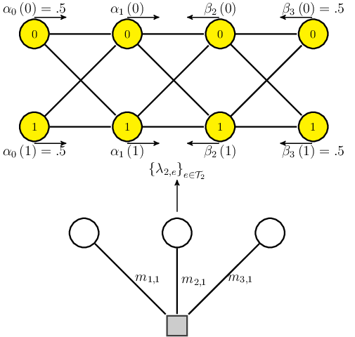
In Section II, joint LP decoder is presented as an LDPC-code constrained shortest-path problem on the channel trellis. In this section, we develop the iterative solver for the joint-decoding LP. There are few key steps in deriving iterative solution for the joint LP decoding problem. For the first step, given by the primal problem (Problem-P) in Table I, we reformulate the original LP (1) in Theorem 13 using only equality constraints involving the indicator variables44 4 The valid patterns for each parity-check allow us to define the indicator variables (for and ) which equal 1 if the codeword satisfies parity-check using configuration and . The second step, given by the 1st formulation of the dual problem (Problem-D1) in Table II, follows from standard convex analysis (e.g., see [42, p. 224]). Strong duality holds because the primal problem is feasible and bounded. Therefore, the Lagrangian dual of Problem-P is equivalent to Problem-D1 and the minimum of Problem-P is equal to the maximum of Problem-D1. From now on, we consider Problem-D1, where the code and trellis constraints separate into two terms in the objective function. See Fig. 3 for a diagram of the variables involved.
The third step, given by the 2nd formulation of the dual problem (Problem-D2) in Table III, observes that forward/backward recursions can be used to perform the optimization over and remove one of the dual variable vectors. This splitting is enabled by imposing the trellis flow normalization constraint in Problem-P only at one time instant . This detail gives different ways to write the same LP and is an important part of obtaining update equations similar to those of TE.
Lemma 24.
Problem-D1 is equivalent to Problem-D2.
Proof:
By rewriting the inequality constraint in Problem-D1 as
we obtain the recursive upper bound for as
This upper bound is achieved by the forward Viterbi update in Problem-D2 for Again, by expressing the same constraint as
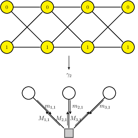
we get a recursive upper bound for . Similar reasoning shows this upper bound is achieved by the backward Viterbi update in Problem-D2 for See Fig. 4 for a graphical depiction of this. ∎The fourth step, given by the softened dual problem (Problem-DS) in Table IV, is formulated by replacing the minimum operator in Problem-D2 with the soft-minimum operation
This smooth approximation converges to the minimum function as increases [32]. Since the soft-minimum function is used in two different ways, we use different constants, and for the code and trellis terms. The smoothness of Problem-DS allows one to to take derivative of (4) (giving the Karush–Kuhn–Tucker (KKT) equations, derived in Lemma 25), and represent (5) and (6) using BCJR-like forward/backward recursions (given by Lemma 26).
where is defined for by
and is defined for by
starting from

| (4) | |||
where is the indicator function of the set is defined for by
| (5) |
and is defined for by
| (6) |
starting from
Lemma 25.
Consider the KKT equations associated with performing the minimization in (4) only over the variables . These equations have a unique solution given by
for where
Proof:
See Appendix A-A.∎
Lemma 26.
Proof:
By letting, , we obtain the desired result by normalization. ∎Now, we have all the pieces to complete the algorithm. As the last step, we combine the results of Lemma 25 and 26 to obtain the iterative solver for the joint-decoding LP, which is summarized by the iterative joint LP decoding in Algorithm 1 (see Fig. 5 for a graphical depiction).
Remark 27.
While Algorithm 1 always has a bit-node update rule different from standard belief propagation (BP), we note that setting in the inner loop gives the exact BP check-node update and setting in the outer loop gives the exact BCJR channel update. In fact, one surprising result of this work is that such a small change to the BCJR-based TE update provides an iterative solver for the LP whose per-iteration complexity similar to TE. It is also possible to prove the convergence of a slightly modified iterative solver that is based on a less efficient update schedule.
- •
Step 1. Initialize for and
- •
Step 2. Update Outer Loop: For ,
- –
(i) Compute bit-to-trellis message
where
- –
(ii) Compute forward/backward trellis messages
(7) (8) where for all .
- –
(iii) Compute trellis-to-bit message
(9)
- –
- •
Step 3. Update Inner Loop for rounds: For ,
- –
(i) Compute bit-to-check msg for
- –
(ii) Compute check-to-bit msg for
(10) where
(11)
- –
- •
Step 4. Compute hard decisions and stopping rule
- –
(i) For ,
- –
(ii) If satisfies all parity checks or the maximum outer iteration number, , is reached, stop and output . Otherwise increment and go to Step 2.
- –
III-B Convergence Analysis
This section considers the convergence properties of Algorithm 1. Although simulations have not shown any convergence problems with Algorithm 1 in its current form, our proof requires a modified update schedule that is less computationally efficient. Following Vontobel’s approach in [32], which is based on general properties of Gauss-Seidel-type algorithms for convex minimization, we show that the modified version Algorithm 1 is guaranteed to converge. Moreover, a feasible solution to Problem-P can be obtained whose value is arbitrarily close to the optimal value of Problem-P.
The modified update rule for Algorithm 1 consists of cyclically, for each , computing the quantity (via step 2 of Algorithm 1) and then updating for all (based on step 3 of Algorithm 1). The drawback of this approach is that one BCJR update is required for each bit update, rather than for bit updates. This modification allows us to interpret Algorithm 1 as a Gauss-Seidel-type algorithm. We believe that, at the expense of a longer argument, the convergence proof can be extended to a decoder which uses windowed BCJR updates (e.g., see [43]) to achieve convergence guarantees with much lower complexity. Regardless, the next few lemmas and theorems can be seen as a natural generalization of [32][36] to the joint-decoding problem.
subject to the same constraints as Problem-P.
Lemma 28.
Assume that all the rows of have Hamming weight at least 3. Then, the modified Algorithm 1 converges to the maximum of the Problem-DS.
Proof:
See Appendix A-B. ∎Next, we introduce the softened primal problem (Problem-PS) in Table V, using the definitions and . Using standard convex analysis (e.g., see [42, p. 254, Ex. 5.5]), one can show that Problem-PS is the Lagrangian dual of Problem-DS and that the minimum of Problem-PS is equal to the maximum of Problem-DS. In particular, Problem-PS can be seen as a maximum-entropy regularization of Problem-DS that was derived by smoothing dual problem given by Problem-D2. Thus, our Algorithm 1 is dually-related to an interior-point method for solving the LP relaxation of joint ML decoding on trellis-wise polytope using the entropy function (for in the standard simplex)
| (12) |
as a barrier function (e.g., see [38, p. 126]) for the polytope.
Remark 29.
Next, we develop a relaxation bound, given by Lemma 30 and Lemma 31 to quantify the performance loss of Algorithm 1 (when it converges) in relation to the joint LP decoder.
Lemma 30.
Let be the minimum value of Problem-P and be the minimum value of Problem-PS. Then
where
and
Proof:
See Appendix A-C.∎
Lemma 31.
For any , the modified Algorithm 1 returns a feasible solution for Problem-DS that satisfies the KKT conditions within . With this, one can construct a feasible solution for Problem-PS that has the (nearly optimal) value . For small enough , one finds that
where
Proof:
Theorem 32.
For any , there exists a sufficiently small and sufficiently large and such that finitely many iterations of the modified Algorithm 1 can be used to construct a feasible for Problem-PS that is also nearly optimal. The value of this solution is denoted and satisfies
where
Proof:
Remark 33.
The modified (i.e., cyclic schedule) Algorithm 1 is guaranteed to converge to a solution whose value can be made arbitrarily close to Therefore, the joint iterative LP decoder provides an approximate solution to Problem-P whose value is governed by the upper bound in Theorem 32. Algorithm 1 can be further modified to be of Gauss-Southwell type so that the complexity analysis in [36] can be extended to this case. Still, the analysis in [36], although a valid upper bound, does not capture the true complexity of decoding because one must choose to guarantee that the iterative LP solver finds the true minimum. Therefore, the exact convergence rate and complexity analysis of Algorithm 1 is left for future study. In general, the convergence rate of coordinate-descent methods (e.g., Gauss-Seidel and Gauss-Southwell type algorithms) for convex problems without strict convexity is an open problem.
IV Error Rate Prediction and Validation
In this section, we validate the proposed joint-decoding solution and discuss some implementation issues. Then, we present simulation results and compare with other approaches. In particular, we compare the performance of the joint LP decoder and joint iterative LP decoder with the joint iterative message-passing decoder on two finite-state intersymbol interference channels (FSISCs) described in Definition 7. For preliminary studies, we use a -regular binary LDPC code on the precoded dicode channel (pDIC) with length 155 and 455. For a more practical scenario, we also consider a -regular binary LDPC code with length 4923 and rate 8/9 on the class-II Partial Response (PR2) channel used as a partial-response target for perpendicular magnetic recording. All parity-check matrices were chosen randomly except that double-edges and four-cycles were avoided. Since the performance depends on the transmitted codeword, the WER results were obtained for a few chosen codewords of fixed weight. The weight was chosen to be roughly half the block length, giving weights 74, 226, and 2462 respectively.
The performance of the three algorithms was assessed based on the following implementation details.
Joint LP Decoder
Joint LP decoding is performed in the dual domain because this is much faster than the primal domain when using MATLAB. Due to the slow speed of LP solver, simulations were completed up to a WER of roughly on the three different non-zero LDPC codes with block lengths 155 and 455 each. To extrapolate the error rates to high SNR (well beyond the limits of our simulation), we use a simulation-based semi-analytic method with a truncated union bound (see (3)) as discussed in Section II. The idea is to run a simulation at low SNR and keep track of all observed codeword and pseudo-codeword (PCW) errors and a truncated union bound is computed by summing over all observed errors. The truncated union bound is obtained by computing the generalized Euclidean distances associated with all decoding errors that occurred at some low SNR points (e.g., WER of roughly than ) until we observe a stationary generalized Euclidean distance spectrum. It is quite easy, in fact, to store these error events in a list which is finally pruned to avoid overcounting. Of course, low SNR allows the decoder to discover PCWs more rapidly than high SNR and it is well-known that the truncated bound should give a good estimate at high SNR if all dominant joint decoding PCWs have been found (e.g., [44, 45]). One nontrivial open question is the feasibility and effectiveness of enumerating error events for long codes. In particular, we do not address how many instances must be simulated to have high confidence that all the important error events are found so there are no surprises at high SNR.
Joint Iterative LP Decoder
Joint iterative decoding is performed based on the Algorithm 1 on all three LDPC codes of different lengths. For block lengths 155 and 455, we chose the codeword which shows the worst performance for the joint LP decoder experiments. We used a simple scheduling update scheme: variables are updated according to Algorithm 1 with cyclically with inner loop iterations for each outer iteration. The maximum number of outer iterations is , so the total iteration count, , is at most 200. The choice of parameters are and on the LDPC codes with block lengths 155 and 455. For the LDPC code with length 4923, is reduced to 10. To prevent possible underflow or overflow, a few expressions must be implemented carefully. When
a well-behaved approximation of (10) and (11) is given by
where is the usual sign function. Also, (9) should be implemented using
where and
Joint Iterative Message-Passing Decoder
Joint iterative message decoding is performed based on the state-based algorithm described in [43] on all three LDPC codes of different lengths. To make a fair comparison with the Joint Iterative LP Decoder, the same maximum iteration count and the same codewords are used.
IV-A Results
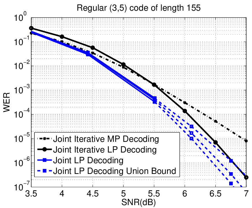
Fig. 6 compares the results of all three decoders and the error-rate estimate given by the union bound method discussed in Section II. The solid lines represent the simulation curves while the dashed lines represent a truncated union bound for three different non-zero codewords. Surprisingly, we find that joint LP decoder outperforms joint iterative message passing decoder by about 0.5 dB at WER of . We also observe that that joint iterative LP decoder loses about 0.1 dB at low SNR. This may be caused by using finite values for and . At high SNR, however, this gap disappears and the curve converges towards the error rate predicted for joint LP decoding. This shows that joint LP decoding outperforms belief-propagation decoding for short length code at moderate SNR with the predictability of LP decoding. Of course, this can be achieved with a computational complexity similar to turbo equalization.
One complication that must be discussed is the dependence on the transmitted codeword. Computing the bound is complicated by the fact that the loss of channel symmetry implies that the dominant PCWs may depend on the transmitted sequence. It is known that long LDPC codes with joint iterative decoding experience a concentration phenomenon [43] whereby the error probability of a randomly chosen codeword is very close, with high probability, to the average error probability over all codewords. This effect starts to appear even at the short block lengths used in this example. More research is required to understand this effect at moderate block lengths and to verify the same effect for joint LP decoding.
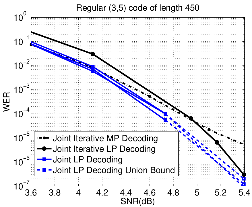
Fig. 7 compares the joint iterative LP decoder and joint iterative message-passing decoder in a practical scenario. Again, we find that the joint iterative LP decoder provides gains over the joint iterative message-passing decoder at high SNR. The slope difference between the curves also suggests that the performance gains of joint iterative LP decoder will increase with SNR. This shows that joint iterative LP decoding can provide performance gains at high SNR with a computational complexity similar to that of turbo equalization.

V Conclusions
In this paper, we consider the problem of linear-programming (LP) decoding of low-density parity-check (LDPC) codes and finite-state channels (FSCs). First, we present an LP formulation of joint-decoding for LDPC codes on FSCs that offers decoding performance improvements over joint iterative message-passing decoding at moderate SNR. Then, joint-decoding pseudo-codewords (JD-PCWs) are defined and the decoder error rate is upper bounded by a union bound over JD-PCWs that is evaluated for deterministic ISI channels with AWGN. Next, we propose a simulation-based semi-analytic method for estimating the error rate of LDPC codes on finite-state intersymbol interference channel (FSISIC) at high SNR using only simulations at low SNR. Finally, we present a novel iterative solver for the joint LP decoding problem. This greatly reduces the computational complexity of the joint LP solver by exploiting the LP dual problem structure. Its main advantage is that it provides the predictability of LP decoding and significant gains over turbo equalization (TE) especially in the error-floor with a computational complexity similar to TE.
Appendix A Proof Details
A-A Proof of Lemma 25
A-B Proof of Lemma 28
To characterize the convergence of the iterative joint LP decoder, we consider the modification of Algorithm 1 with cyclic updates. The analysis follows [32] and uses the proposition about convergence of block coordinate descent methods from [46, p. 247].
Proposition 34.
Consider the problem
where and each is a closed convex subset of . The vector is partitioned so with . Suppose that is continuously differentiable and convex on and that, for every and every , the problem
has a unique minimum. Now, consider the sequence defined by
for . Then, every limit point of this sequence minimizes over
By using Proposition 34, we will show that the modified Algorithm 1 converges. Define and
Let us consider cyclic coordinate decent algorithm which minimizes cyclically with respect to the coordinate variable. Thus is changed first, then and so forth through Then (4), (5), and (6) are equivalent to for each with proper as
Using the properties of log-sum-exp functions (e.g., see [42, p. 72]), one can verify that is continuously differentiable and convex. The minimum over for all is uniquely obtained because of the unique KKT solution in Lemma 25. Therefore, we can apply the Proposition 34 to achieve the desired convergence result under the modified update schedule. It is worth mentioning that the Hamming weight condition prevents degeneracy of Problem-DS based on the fact that, otherwise, some pairs of bits must always be equal.
A-C Proof of Lemma 30
Denote the optimum solution of Problem-P by and and the optimum solution of Problem-PS by and Since and are the optimal with respect to the Problem-P, we have
| (16) |
On the other hand, and are the optimal with respect to the Problem-PS, we have
where is the entropy defined by (12). We rewrite this as
| (17) |
The last inequality is due to nonnegativity of entropy. Using Jensen’s inequality, we obtain
| (18) |
and
| (19) |
By substituting (18) and (19) to (17), we have
| (20) |
A-D Proof of Lemma 31
For the coordinate-descent solution of Problem-DS, minimizing over the -th block gives
| (21) |
subject to
The solution can be obtained by applying the KKT conditions and this yields
| (22) |
Given a feasible solution of the modified Algorithm 1, we define
with
and
Suppose we stop iterating when and define
where
First, we claim that This is because setting
| (23) |
obviously satisfies for
and satisfies for
From [36, p. 4841], it follows that . Next, we show that Note that defining
implies that (by (14))
obviously satisfies for
Furthermore,
and by Definition 8, . Therefore, we conclude that is feasible in Problem-P. From [36, p. 4855], it follows that there exist feasible vectors associated with .
Denote the minimum value of Problem-PS by Then by the Lagrange duality we can upper bound with
where is given by rewriting (23) as
The last step of this equation follows from
In the above equation, the details of the last two inequalities are not included due to space limitations, but they can be derived using arguments very similar to [36, p. 4840-4841].
References
- [1] C. Douillard, M. Jézéquel, C. Berrou, A. Picart, P. Didier, and A. Glavieux, “Iterative correction of intersymbol interference: Turbo equalization,” Eur. Trans. Telecom., vol. 6, no. 5, pp. 507–511, Sept. – Oct. 1995.
- [2] R. G. Gallager, “Low-density parity-check codes,” Ph.D. dissertation, M.I.T., Cambridge, MA, USA, 1960.
- [3] R. R. Müller and W. H. Gerstacker, “On the capacity loss due to separation of detection and decoding,” IEEE Trans. Inform. Theory, vol. 50, no. 8, pp. 1769–1778, Aug. 2004.
- [4] W. E. Ryan, “Performance of high rate turbo codes on a PR4-equalized magnetic recording channel,” in Proc. IEEE Int. Conf. Commun. Atlanta, GA, USA: IEEE, June 1998, pp. 947–951.
- [5] L. L. McPheters, S. W. McLaughlin, and E. C. Hirsch, “Turbo codes for PR4 and EPR4 magnetic recording,” in Proc. Asilomar Conf. on Signals, Systems & Computers, Pacific Grove, CA, USA, Nov. 1998.
- [6] M. Öberg and P. H. Siegel, “Performance analysis of turbo-equalized dicode partial-response channel,” in Proc. 36th Annual Allerton Conf. on Commun., Control, and Comp., Monticello, IL, USA, Sept. 1998, pp. 230–239.
- [7] M. Tüchler, R. Koetter, and A. Singer, “Turbo equalization: principles and new results,” IEEE Trans. Commun., vol. 50, no. 5, pp. 754–767, May 2002.
- [8] B. M. Kurkoski, P. H. Siegel, and J. K. Wolf, “Joint message-passing decoding of LDPC codes and partial-response channels,” IEEE Trans. Inform. Theory, vol. 48, no. 6, pp. 1410–1422, June 2002.
- [9] G. Ferrari, G. Colavolpe, and R. Raheli, Detection Algorithms for Wireless Communications, with Applications to Wired and Storage Systems. John Wiley & Sons, Ltd, 2004.
- [10] A. Dholakia, E. Eleftheriou, T. Mittelholzer, and M. Fossorier, “Capacity-approaching codes: can they be applied to the magnetic recording channel?” IEEE Commun. Magazine, vol. 42, no. 2, pp. 122 –130, Feb. 2004.
- [11] A. Anastasopoulos, K. Chugg, G. Colavolpe, G. Ferrari, and R. Raheli, “Iterative detection for channels with memory,” Proceedings of the IEEE, vol. 95, no. 6, pp. 1272–1294, June 2007.
- [12] A. Kavčić and A. Patapoutian, “The read channel,” Proceedings of the IEEE, vol. 96, no. 11, pp. 1761–1774, Nov. 2008.
- [13] J. Feldman, “Decoding error-correcting codes via linear programming,” Ph.D. dissertation, M.I.T., Cambridge, MA, 2003.
- [14] J. Feldman, M. J. Wainwright, and D. R. Karger, “Using linear programming to decode binary linear codes,” IEEE Trans. Inform. Theory, vol. 51, no. 3, pp. 954–972, March 2005.
- [15] [Online]. Available: http://www.PseudoCodewords.info
- [16] P. Vontobel and R. Koetter, “Graph-cover decoding and finite-length analysis of message-passing iterative decoding of LDPC codes,” Dec. 2005, [Online]. Available: http://arxiv.org/abs/cs/0512078.
- [17] B.-H. Kim and H. D. Pfister, “On the joint decoding of LDPC codes and finite-state channels via linear programming,” in Proc. IEEE Int. Symp. Inform. Theory, Austin, TX, June 2010, pp. 754–758.
- [18] M. F. Flanagan, “Linear-programming receivers,” in Proc. 47th Annual Allerton Conf. on Commun., Control, and Comp., Monticello, IL, Sept. 2008, pp. 279–285.
- [19] ——, “A unified framework for linear-programming based communication receivers,” Feb. 2009, [Online]. Available: http://arxiv.org/abs/0902.0892.
- [20] B.-H. Kim and H. D. Pfister, “An iterative joint linear-programming decoding of LDPC codes and finite-state channels,” in Proc. IEEE Int. Conf. Commun., June 2011, To appear, available: http://arxiv.org/abs/1009.4352.
- [21] K. A. S. Immink, P. H. Siegel, and J. K. Wolf, “Codes for digital recorders,” IEEE Trans. Inform. Theory, vol. 44, no. 6, pp. 2260–2299, Oct. 1998.
- [22] S. Jeon, X. Hu, L. Sun, and B. Kumar, “Performance evaluation of partial response targets for perpendicular recording using field programmable gate arrays,” IEEE Trans. Magn., vol. 43, no. 6, pp. 2259–2261, 2007.
- [23] M. F. Flanagan, V. Skachek, E. Byrne, and M. Greferath, “Linear-programming decoding of nonbinary linear codes,” IEEE Trans. Inform. Theory, vol. 55, no. 9, pp. 4134–4154, Sept. 2009.
- [24] M. H. Taghavi and P. H. Siegel, “Graph-based decoding in the presence of ISI,” IEEE Trans. Inform. Theory, vol. 57, no. 4, pp. 2188–2202, April 2011.
- [25] T. Wadayama, “Interior point decoding for linear vector channels based on convex optimization,” IEEE Trans. Inform. Theory, vol. 56, no. 10, pp. 4905–4921, Oct. 2010.
- [26] J. Ziv, “Universal decoding for finite-state channels,” IEEE Trans. Inform. Theory, vol. 31, no. 4, pp. 453–460, July 1985.
- [27] R. Ash, Information theory. Dover, 1990.
- [28] N. Wiberg, “Codes and decoding on general graphs,” Ph.D. dissertation, Linköping University, S-581 83 Linköping, Sweden, 1996.
- [29] C. Di, D. Proietti, E. Telatar, T. J. Richardson, and R. Urbanke, “Finite-length analysis of low-density parity-check codes on the binary erasure channel,” IEEE Trans. Inform. Theory, vol. 48, no. 6, pp. 1570–1579, June 2002.
- [30] T. Richardson, “Error floors of LDPC codes,” Proc. 42nd Annual Allerton Conf. on Commun., Control, and Comp., Oct. 2003.
- [31] G. D. Forney, Jr., R. Koetter, F. R. Kschischang, and A. Reznik, “On the effective weights of pseudocodewords for codes defined on graphs with cycles,” in Codes, systems and graphical models, ser. IMA Volumes Series, B. Marcus and J. Rosenthal, Eds., vol. 123. New York: Springer, 2001, pp. 101–112.
- [32] P. Vontobel and R. Koetter, “Towards low-complexity linear-programming decoding,” in Proc. Int. Symp. on Turbo Codes & Related Topics, Munich, Germany, April 2006.
- [33] P. Vontobel, “Interior-point algorithms for linear-programming decoding,” in Proc. 3rd Annual Workshop on Inform. Theory and its Appl., San Diego, CA, Feb. 2008.
- [34] M. Taghavi and P. Siegel, “Adaptive methods for linear programming decoding,” IEEE Trans. Inform. Theory, vol. 54, no. 12, pp. 5396–5410, Dec. 2008.
- [35] T. Wadayama, “An LP decoding algorithm based on primal path-following interior point method,” in Proc. IEEE Int. Symp. Inform. Theory, Seoul, Korea, June 2009, pp. 389–393.
- [36] D. Burshtein, “Iterative approximate linear programming decoding of LDPC codes with linear complexity,” IEEE Trans. Inform. Theory, vol. 55, no. 11, pp. 4835–4859, Nov. 2009.
- [37] M. Punekar and M. F. Flanagan, “Low complexity linear programming decoding of nonbinary linear codes,” in Proc. 48th Annual Allerton Conf. on Commun., Control, and Comp., Monticello, IL, Sept. 2010.
- [38] J. K. Johnson, “Convex relaxation methods for graphical models: Lagrangian and maximum entropy approaches,” Ph.D. dissertation, M.I.T., Cambridge, MA, 2008.
- [39] P. Regalia and J. Walsh, “Optimality and duality of the turbo decoder,” Proceedings of the IEEE, vol. 95, no. 6, pp. 1362–1377, 2007.
- [40] F. Alberge, “Iterative decoding as Dykstra’s algorithm with alternate i-projection and reverse i-projection,” in Proc. Eur. Signal Process. Conf., Lausanne, Switzerland, 2008.
- [41] J. Walsh and P. Regalia, “Belief propagation, Dykstra’s algorithm, and iterated information projections,” IEEE Trans. Inform. Theory, vol. 56, no. 8, pp. 4114–4128, 2010.
- [42] S. Boyd and L. Vandenberghe, Convex Optimization. Cambridge University Press, 2004.
- [43] A. Kavčić, X. Ma, and M. Mitzenmacher, “Binary intersymbol interference channels: Gallager codes, density evolution and code performance bounds,” IEEE Trans. Inform. Theory, vol. 49, no. 7, pp. 1636–1652, July 2003.
- [44] X. Hu, Z. Li, V. Kumar, and R. Barndt, “Error floor estimation of long LDPC codes on magnetic recording channels,” IEEE Trans. Magn., vol. 46, no. 6, pp. 1836–1839, June 2010.
- [45] P. Lee, L. Dolecek, Z. Zhang, V. Anantharam, B. Nikolic, and M. Wainwright, “Error floors in LDPC codes: Fast simulation, bounds and hardware emulation,” in Proc. IEEE Int. Symp. Inform. Theory, Toronto, Canada, July 2008, pp. 444–448.
- [46] D. Bertsekas, Nonlinear Programming. Athena Scientific Belmont, MA, 1995.