Collapse of ultrashort spatiotemporal pulses described by the cubic generalized Kadomtsev-Petviashvili equation
Abstract
By using a reductive perturbation method, we derive from Maxwell-Bloch equations, a cubic generalized Kadomtsev-Petviashvili equation for ultrashort spatiotemporal optical pulse propagation in cubic (Kerr-like) media, without the use of the slowly varying envelope approximation. We calculate the collapse threshold for the propagation of few-cycle spatiotemporal pulses described by the generic cubic generalized Kadomtsev-Petviashvili equation by a direct numerical method, and compare it to analytic results based on a rigorous virial theorem. Besides, typical evolution of the spectrum (integrated over the tranverse spatial coordinate) is given and a strongly asymmetric spectral broadening of ultrashort spatiotemporal pulses during collapse is evidenced.
pacs
42.65.Tg, 42.65.Re, 05.45.YvI Introduction
The rapid progress over the past two decades in the area of ultrafast optics has led to the production, manipulation and control of pulses with durations down to a few optical cycles (see, e.g., the comprehensive review [1]). The theoretical and experimental studies of few-cycle pulses (FCPs) have opened the door to a series of applications in various fields such as light matter interaction, high-order harmonic generation, extreme nonlinear optics [2], and attosecond physics [3, 4]. On the theoretical arena three classes of main dynamical models for FCPs have been put forward: (i) the quantum approach [5, 6, 7, 8], (ii) the refinements within the framework of the slowly varying envelope approximation (SVEA) of the nonlinear Schrödinger-type envelope equations [9, 10, 11, 12], and non-SVEA models [13, 14, 15, 16, 17]. In media with cubic (Kerr-type) optical nonlinearity the physics of (1+1)-dimensional FCPs can be adequately described beyond the SVEA by using different dynamical models, such as the modified Korteweg-de Vries (mKdV) [13], sine-Gordon (sG) [14, 15], or mKdV-sG equations [16, 17, 18]. It is worthy to notice that the physics of the (1+1)-dimensional FCPs is well described by the generic mKdV-sG equation [16]; this quite general model was also derived and studied in Refs. [19, 20].
Another class of conceptually important optical problems for which the SVEA approach does not apply in the femtosecond regime includes multidimensional spatiotemporal optical solitons (alias “light bullets”), formed by the competing diffraction, dispersion, and quadratic [21] or cubic [22] nonlinearity. Thus for the adequate description of multidimensional FCPs, a non-integrable generalized Kadomtsev-Petviashvili (KP) equation [23] (a two-dimensional version of the mKdV model) was introduced for (2+1)-dimensional few-optical-cycle spatiotemporal soliton propagation in cubic nonlinear media beyond the SVEA [24, 25]. Recently, by using a powerful reductive perturbation technique [26], or a multiscale analysis, a generic KP evolution equation governing the propagation of femtosecond spatiotemporal optical solitons in quadratic nonlinear media beyond the SVEA was also put forward [27].
Transparency of the medium is obviously required by soliton propagation. It implies that all transition frequencies of the medium are far from the typical frequency of the wave. They can be either well above or well below the latter. As shown in (1+1) dimensions [14], a wave frequency much lower than the resonance frequency corresponds to a long wave approximation and to a mKdV model, while a wave frequency much higher than it corresponds to a short wave approximation and a sG model. Later, a generic mKdV-sG model has been derived for the case of two transition lines, one well above, and the other one well below the wave frequency [16], and is the most general non-SVEA model proposed to describe FCP propagation in Kerr media [18]. It is expected to remain valid in the general case, where two sets of resonance lines are present instead of two single transitions. Our ultimate goal is to generalize the generic mKdV-sG model to (2+1) dimensions. However, both long- and short wave approximations for a simple two-level model have not yet been rigorously derived. It might be relevant to consider the full set of atomic levels, and it would be necessary in order to compute the nonlinear coefficients in a quantitative way. However, as a preliminary approach and for the sake of tractability, we need to consider a simplified model, but a natural question arises, why we consider a two-level model and not, e.g., a four-level one? As written above, it has been previously shown [14, 16] that if we consider only two separate transitions, one with resonance frequency below the optical range, and the second one above it, the FCP propagation is considerably affected. The most relevant refinement of the two-level model is thus a level one. Our preliminary computations for the model of two sets of two levels show that in the long wave approximation considered in the present work, both the dispersive and the nonlinear coefficients merely sum up. In fact, we expect that the model equation obtained for the complete model with arbitrary number of levels, when all resonance lines are well above the wave frequency, has the same form as the one derived for the two-level model, only with modified values of nonlinear coefficients. However, this is not the case when the resonance line is well below the wave frequency, since the pulse evolution involves the difference of populations between the levels in a nonlinear way. In this situation, we expect a more complicated evolution equation for FCPs when more than two levels are involved. This general model, which might be, in our opinion, the most relevant correction to the two-level model, is left for further investigation. On the other hand, the two-level system has many interesting features by itself: It is in some sense equivalent to a classical oscillator, as can be shown from the computation of the nonlinear susceptibilities [28], or from the derivation of the KdV model for FCPs propagation in quadratic nonlinear media [29]. Moreover, estimations of the value of the nonlinear coefficient drawn from the classical model have shown a very good agreement with experimental data, as, e.g., in the case of the model developed in Ref. [30].
Thus there are three main issues which deserve to be investigated: the first one, which constitutes the aim of the present manuscript, is the long-wave approximation leading to the cubic generalized Kadomtsev-Petviashvili (CGKP) equation, which yields collapse. The second and the third worth studying open problems are, respectively, the short wave approximation and the investigation of the full model with both mKdV and sG terms. On this ground, we consider that the study of the CGKP model, including the derivation of the CGKP equation from a two-level model, is an important step in the adequate description of (2+1)-dimensional FCPs.
The aim of this paper is to derive and to study a cubic generalized Kadomtsev-Petviashvili partial differential equation, which describes the dynamics of (2+1)-dimensional spatiotemporal pulses in cubic nonlinear media beyond the SVEA model equations, starting from the Maxwell-Bloch equations for a set of two-level atoms. This paper is organized as follows. In Sec. II we derive the generic CGKP equation and we study by adequate numerical methods the propagation dynamics, the nonlinear difraction and, in the case of anomalous dispersion, the collapse of ultrashort spatiotemporal pulses. We calculate in Sec. III the collapse threshold for the propagation of ultrashort spatiotemporal pulses described by the CGKP equation by both a direct numerical method and by an analytical method, which is based on a rigorous virial theorem. In Sec. IV, the evolution of the spectrum (integrated over the transverse coordinate) is given and a strongly asymmetric spectral broadening of ultrashort pulses during collapse is put into evidence. Section V presents our conclusions.
II The cubic generalized Kadomtsev-Petviashvili equation and its numerical computation
For a Kerr (cubic) medium a CGKP equation can be derived from Maxwell-Bloch equations using the powerful reductive perturbation method [26]. As said in the introduction, we consider a set of two-level atoms with the Hamiltonian
| (1) |
where is the frequency of the transition. The evolution of the electric field is described by the wave equation
| (2) |
where is the polarization density. The light propagation is coupled with the medium by means of a dipolar electric momentum
| (3) |
directed along the same direction as the electric field, according to
| (4) |
and the polarization density along the -direction is
| (5) |
where is the volume density of atoms and the density matrix. Since, as shown in [14], the relaxation can be neglected, the density-matrix evolution equation (Schrödinger equation) reduces to
| (6) |
Transparency implies that the characteristic frequency of the considered radiation (in the optical range) strongly differs from the resonance frequency of the atoms. Here, as explained in the introduction, we assume that is much smaller than . This motivates the introduction of the slow variables
| (7) |
being a small parameter. The delayed time involves propagation at some speed to be determined. It is assumed to vary slowly in time according to the assumption . The pulse shape described by the variable evolves even more slowly in time, the corresponding scale being that of variable . The transverse spatial variable has an intermediate scale as usual in KP-type expansions [26].
Next we use the reductive perturbation method as developed in Ref. [26]. To this aim we expand the electric field as power series of a small parameter :
| (8) |
as in the standard mKdV-type expansions [26]. A weak amplitude assumption is needed in order that the nonlinear effects arise at the same propagation distance scale as the dispersion does, which justifies that the expansion of begins at order . The polarization density is expanded in the same way.
The expansion [Eqs. (7) and (8)] is then reported into the basic equations [Eqs. (1-6)], and solved order by order. The computation is very close to the (1+1)-dimensional case (see Ref. [14]) in what concerns nonlinearity and dispersion, while the treatment of dispersion and the dependency with respect to the transverse (spatial) variable is fully analogous to the case of quadratic nonlinear media, see Ref. [27]. As a result we get the model equation
| (9) |
which is a CGKP equation. The dispersion and nonlinear coefficients and in the above (2+1)-dimensional evolution equation are
| (10) |
respectively, the refractive index being
| (11) |
The CGKP model equation (9) is generalized by expressing the coefficients and in terms of dispersion relation and third-order nonlinear susceptibility . They can indeed be written as
| (12) |
| (13) |
Also, the coefficient in Eq. (9) is the group velocity, .
By means of an adequate linear rescaling, the CGKP equation (9) can be reduced to the normalized form
| (14) |
where and . In the frame of the Maxwell-Bloch equations, , hence the nonlinearity and dispersion yield temporal self-compression, but nonlinearity and diffraction tend to defocuse the FCP.
The CGKP equation (14) is solved by means of the fourth order Runge Kutta exponential time differencing (RK4ETD) scheme [31]. It involves one integration with respect to . The inverse derivative is computed by means of a Fourier transform, which implies that the integration constant is fixed so that the mean value of the inverse derivative is zero, but also that the linear term is replaced with zero, i.e., the mean value of the function is set to zero. For low frequencies, the coefficients of the RK4ETD scheme are computed by means of series expansions, to avoid catastrophic consequences of limited numerical accuracy.
We consider in our simulations input data in the form
| (15) |
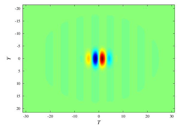
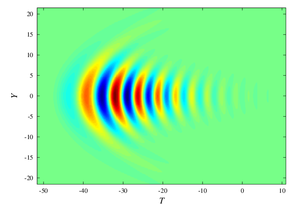
Setting as pertains to the Maxwell-Bloch system, we observe nonlinear diffraction (Fig. 1). The nonlinear effect strongly increases the diffraction (compare Figs. 1c and d). The conjugated effect of temporal self-compression and diffraction may lead to an intermediary stage, in which the pulse is very well localized temporally, and strongly widens spatially. This leads to a characteristic crescent shape (Fig. 1b). For the computations we used the parameters , , , and .


The CGKP equation (9) can be generalized using the expressions (12) and (13) of the coefficients. For a medium with anomalous dispersion and focusing nonlinearity, and . In this case spatiotemporal self-focusing occurs.


Numerical resolution has been performed for , , , and for several values of the initial amplitude , especially , 3.65, 3.57, and 3.50. Clear numerical evidence for collapse is found, see Figs. 2 and 3. Collapse occurs for the two highest values of the input spatiotemporal field amplitudes (curves and in Fig. 2), and not for the two lowest ones (curves and in Fig. 2). Hence the occurence of some input amplitude threshold is evidenced, and for the considered pulse shape, frequency, length and width, we get the numerical estimation .
On the other hand, a rigorous mathematical analysis of the CGKP equation (9) has proved that wave collapse do occurs (for a comprehensive review of wave collapse in optics and plasma waves, see Ref. [32]); also, for more details concerning CGKP equation see Refs. [33]-[36] and the analysis performed in the next Section.
III Calculation of the collapse threshold
In the following let us consider the generalized KP (GKP) equation in its normalized form
| (16) |
The focusing CGKP equation (9) with is obtained for the particular case . The GKP equation possesses the conserved Hamiltonian
| (17) |
in which . Note that the existence of the conserved Hamiltonian assumes that both and vanish at and , which implies that
i.e., that the mean value of the electric field is zero.

Using a virial theorem, it has been proved that collapse occurs for and [33, 34]. However, these conditions are sufficient but not necessary. Then, it was shown that the solitary wave is unstable for [34, 35], and a proof of collapse by using a virial theorem was given in Ref. [36] for , which includes the particular case , which is relevant for the study of few-cycle optical pulses. The assumptions of the theorem involve the functional
| (18) |
Together with regularity conditions and conditions involving the solitary wave solution, the main assumption of the blow-up theorem is that the functional , in which is the initial data. For the expression of given by Eq. (15), the functional can be exactly computed using standard methods, and we get
| (19) | |||||
where Im is the imaginary part and erf is the error function.
The factor which multiplies in the wide bracket in Eq. (19) is always negative, and hence is negative for larger than some threshold value , with
| (20) |
For the specific values of parameters used in our numerical computations, we find that . The threshold found numerically is about half of this value , found using the assumptions of the above mentioned virial theorem, which is consistent with the well-known fact that the conditions of the theorem of Ref. [36], especially , yield only a sufficient condition. The quantity will be referred to below as the ‘analytical threshold for collapse’ for the sake of simplicity.
However, it is likely that this condition is optimal for an input which has a shape adapted to the collapse process. On the basis of this idea and of the numerical results, the discrepancy can be physically interpreted as follows. Figure 4 presents the evolution of the width of the pulse against propagation distance , for a few initial values of input amplitude (see Eq. (15)). The width is numerically computed according to:
It is seen that self-focusing occurs in every case presented in Fig. 4. However, for initial amplitude below threshold , the self-focusing stops after a while and the collapse is inhibited. This feature is due to the dispersion (both linear and nonlinear), which tends to increase the temporal length of the pulse at the same time as it self-focuses. Below the threshold, the dispersion dominates and collapse is prevented, while above the threshold, self-focusing dominates and collapse occurs. It is worthy to mention that the arrest of collapse due to dispersion was already mentioned in Ref. [24].
This observation may justify qualitatively the discrepancy between the analytic and numerical thresholds for collapse found above. Between the two values for threshold (), at the beginning of the process, the amplitude is not properly speaking sufficient to initiate collapse but, due to the shape of the pulse, a nonlinear lens effect induces a transverse self-focusing of the pulse, which increases the maximal pulse amplitude. At the same time, dispersion (linear and nonlinear) occurs, which tends to decrease the amplitude. If dispersion dominates, the growth of the amplitude stops and collapse does not occur. If, on the contrary, self-focusing dominates, the peak amplitude reaches a value which is sufficient to induce the collapse as such. Notice that in Fig. 3, the collapsing curves show two distinct parts, the first one (oscillating) corresponds rather to self-focusing and the second one corresponds rather to collapse stricto sensu. The value of the amplitude at the boundary between the two regions is close to the threshold value for collapse () found from the mathematical condition , see Eqs. (19) and (20).
IV Spectral broadening


The evolution of the spectrum (integrated over ) is shown in Figs. 5 and 6. At the beginning of the evolution process, the spectrum tends to be narrowed. Then the spectrum presents the oscilatory structure typical of the modulation instability (Fig. 6b). However it is strongly asymmetric, in contrast with the case of the ‘long’ pulses described within the SVEA. Finally, a strong broadening of the spectrum is seen as the collapse itself occurs (Fig. 6c).
V Conclusions
In conclusion, we have introduced a model beyond the slowly varying envelope approximation of the comonly used nonlinear Schrödinger-type evolution equations, for describing the propagation of (2+1)-dimensional spatiotemporal ultrashort optical solitons in Kerr (cubic) nonlinear media. Our approach is based on the Maxwell-Bloch equations for an ensemble of two level atoms and on the multiscale approach, and as a result of using the powerful reductive perturbation method [26], a generic cubic generalized Kadomtsev-Petviashvili partial differential evolution equation was put forward. Nonlinearly enhanced diffraction accompanying temporal self-compression is observed. In the case of anomalous dispersion and focusing nonlinearity, collapse is evidenced. The collapse threshold for the propagation of ultrashort spatiotemporal pulses described by the cubic generalized Kadomtsev-Petviashvili equation was calculated numerically, and compared to the analytical results drawn from a theorem based on a virial method, which proves that collapse occurs. The discrepancy between the value of the collapse treshold obtained numerically and the corresponding analytical threshold for collapse is qualitatively explained. Moreover, the evolution of the spectrum (integrated over the transverse, spatial coordinate) is also given and a strongly asymmetric spectral broadening of ultrashort pulses during collapse is also put forward, in contrast to the case of long spatiotemporal pulses described within the slowly varying envelope approximation. The present study is restricted to (2+1) dimensions, however, it can be extended to the (3+1) dimensions [37] by incorporating into the generic model a second transverse (spatial coordinate).
VI Acknowledgment
One of the authors (D.M.) was supported in part by the Romanian Ministry of Education and Research through Grant No. IDEI-497/2009.
References
- [1] T. Brabec and F. Krausz, Rev. Mod. Phys. 72, 545 (2000).
- [2] M. Wegener, Extreme Nonlinear Optics (Springer-Verlag, Berlin, 2005).
- [3] A. Scrinzi, M. Yu. Ivanov, R. Kienberger, and D. M. Villeneuve, J. Phys. B: At. Mol. Opt. Phys. 39, R1 (2006).
- [4] F. Krausz and M. Ivanov, Rev. Mod. Phys. 81, 163 (2009).
- [5] X. Tan, X. Fan, Y. Yang, and D. Tong, J. Mod. Opt. 55, 2439 (2008).
- [6] N. N. Rosanov, V. E. Semenov, and N. V. Vyssotina, Laser Phys. 17, 1311 (2007).
- [7] N. N. Rosanov, V. E. Semenov, and N. V. Vysotina, Quantum Electron. 38, 137 (2008).
- [8] A. Nazarkin, Phys. Rev. Lett. 97, 163904 (2006).
- [9] T. Brabec and F. Krausz, Phys. Rev. Lett. 78, 3282 (1997).
- [10] M. V. Tognetti and H. M. Crespo, J. Opt. Soc. Am. B 24, 1410 (2007).
- [11] A. A. Voronin and A. M. Zheltikov, Phys. Rev. A 78, 063834 (2008).
- [12] A. Kumar and V. Mishra, Phys. Rev. A 79, 063807 (2009).
- [13] I. V. Mel’nikov, D. Mihalache, F. Moldoveanu, and N.-C. Panoiu, Phys. Rev. A 56, 1569 (1997); JETP Lett. 65, 393 (1997).
- [14] H. Leblond and F. Sanchez, Phys. Rev. A 67, 013804 (2003).
- [15] I. V. Mel’nikov, H. Leblond, F. Sanchez, and D. Mihalache, IEEE J. Sel. Top. Quantum Electron. 10, 870 (2004).
- [16] H. Leblond, S. V. Sazonov, I. V. Mel’nikov, D. Mihalache, and F. Sanchez, Phys Rev. A 74, 063815 (2006).
- [17] H. Leblond, I. V. Mel’nikov, and D. Mihalache, Phys. Rev. A 78, 043802 (2008).
- [18] H. Leblond and D. Mihalache, Phys. Rev. A 79, 063835 (2009).
- [19] S. V. Sazonov, JETP 92, 361 (2001).
- [20] A. N. Bugay and S. V. Sazonov, J. Opt. B: Quantum Semiclass. Opt. 6, 328 (2004).
- [21] B. A. Malomed, P. Drummond, H. He, A. Berntson, D. Anderson, and M. Lisak, Phys. Rev. E 56, 4725 (1997); D. V. Skryabin and W. J. Firth, Opt. Commun. 148, 79 (1998); H. Leblond, J. Phys. A 31, 5129 (1998); D. Mihalache, D. Mazilu, B. A. Malomed, and L. Torner, Opt. Commun. 152, 365 (1998); Opt. Commun. 169, 341 (1999); Opt. Commun. 159, 129 (1999); D. Mihalache, D. Mazilu, L.-C. Crasovan, L. Torner, B. A. Malomed, and F. Lederer, Phys. Rev. E 62, 7340 (2000).
- [22] Y. Silberberg, Opt. Lett. 15, 1282 (1990); A. B. Blagoeva, S. G. Dinev, A. A. Dreischuh, and A. Naidenov, IEEE J. Quantum Electron. QE-27, 2060 (1991); M. Desaix, D. Anderson, and M. Lisak, Opt. Lett. 16, 2082 (1991); D. E. Edmundson and R. H. Enns, Opt. Lett. 17, 586 (1992); N. Akhmediev and J. M. Soto-Crespo, Phys. Rev. A 47, 1358 (1993); R. McLeod, K. Wagner, and S. Blair, Phys. Rev. A 52, 3254 (1995).
- [23] B. B. Kadomtsev and V. I. Petviashvili, Dokl. Akad. Nauk SSSR 192, 753 (1970) [Sov. Phys. Dokl. 15, 539 (1970)].
- [24] I. V. Mel’nikov, D. Mihalache, and N.-C. Panoiu, Opt. Commun. 181, 345 (2000).
- [25] H. Leblond, F. Sanchez, I. V. Mel’nikov, and D. Mihalache, Mathematics and Computers in Simulations 69, 378 (2005).
- [26] H. Leblond, J. Phys. B: At. Mol. Opt. Phys. 41, 043001 (2008).
- [27] H. Leblond, D. Kremer, and D. Mihalache, Phys. Rev. A 80, 053812 (2009).
- [28] R. W. Boyd, Nonlinear Optics, Second Edition (Academic Press, New York, 2003).
- [29] H. Leblond, Phys. Rev. A 78, 013807 (2008).
- [30] N. L. Boling, A. J. Glass, and A. Owyoung, IEEE J. Quantum Electron. QE-14, 601 (1978).
- [31] S. M. Cox and P. C. Matthews, J. Comput. Phys. 176, 430 (2002).
- [32] L. Berge, Phys. Rep. 303, 260 (1998).
- [33] S. K. Turitsyn and G. E. Fal’kovitch, Sov. Phys. J.E.T.P. 62, 146 (1985).
- [34] X. P. Wang, M. J. Ablowitz and H. Segur, Physica D 78, 241 (1994).
- [35] A. de Bouard and J.-C. Saut, Contemporary Mathematics 200, 75 (1996).
- [36] Y. Liu, Transactions of the American Mathematical Society 353, 191 (2000).
- [37] B. A. Malomed, D. Mihalache, F. Wise, and L. Torner, J. Opt. B: Quantum Semiclassical Opt. 7, R53 (2005).