Discriminating Different $Z^{\prime}$s via Asymmetries at the LHC

In order to illustrate the $Z^{\prime}$ contribution to asymmetry, we describe firstly the forward-backward (FB) asymmetry in the SM. At the tree level in the SM, the FB asymmetry of $q\bar{q}\rightarrow Z/\gamma^{*}\rightarrow l\bar{l}$ gets contributions from the self conjugation of the Z-induced s-channel feynman diagram

and the interference between this diagram and the $\gamma$-induced s-channel feynman diagram

Around the Z-pole, the FB asymmetry is almost determined by the first contribution, while off the Z-pole, the second contribution plays an important role.

After introducing $Z^{\prime}$, the situation becomes a little bit complicated. On the $Z^{\prime}$ pole, if the coupling of the $Z^{\prime}$ to fermions is not pure vector-like nor pure axial-vector-like namely $|g_{L}^{f}|=|g_{R}^{f}|$, there will be non-zero contribution to FB asymmetry from the self-conjugation of the $Z^{\prime}$ induced s-channel feynman diagram. Otherwise contribution from self-conjugation of $Z^{\prime}$ to F-B asymmetry will be zero. However for the data sample off the $Z^{\prime}$ pole, FB asymmetry will be non-zero due to the interference of the $Z^{\prime}$ diagram and the SM Z/$\gamma^{*}$ induced s-channel feynman diagrams.

From the above description, we can see clearly that the FB asymmetry relates tightly to the chiral properties of the couplings and how to select data samples. In the BSM which contains the $Z^{\prime}$, the coupling of $Z^{\prime}$ and SM fermions is usually different. How to extract the corresponding couplings via asymmetry measurement and subsequently discriminate different BSM is the key motivation for both the theoretical and experimental studies.

The above formulas are applicable also to $q\bar{q}\rightarrow b\bar{b}(t\bar{t})$, however there are additional important contributions to the F-B asymmetry from the QCD high-order processes [29, 30]. If one selects the events around the $Z^{\prime}$ pole, the QCD high-order contributions are suppressed. However such effect will be important for the asymmetry of off-pole events. In this paper, such QCD-induced contributions will be included in the analysis.

The proton-proton collider LHC is forward-backward charge symmetric, so the asymmetry of the fermion pairs produced at the LHC is null if integrating over the full phase space. However, by imposing some kinematical cuts, the asymmetry generated at the partonic level $q\bar{q}\rightarrow f\bar{f}$ can be kept. Different types of asymmetries have been defined. The above-mentioned FB asymmetry [1, 2, 3, 4, 5, 6, 7, 8, 9, 10] which have been frequently used in $Z^{\prime}$ studies contains a characteristic fermion pair rapidity $Y_{{f\bar{f}}}$ cut. We refer it as rapidity dependent forward-backward asymmetry ($\rm{A_{RFB}}$) throughout this paper. The other three asymmetries which will be investigated in this paper are one-side forward-backward asymmetry ($\rm{A_{OFB}}$) [33, 34], central charge asymmetry ($\rm{A_{C}}$) [29, 30, 31, 32], and edge charge asymmetry ($\rm{A_{E}}$) [35]. We collect their definitions as below

in which $Y$ is the rapidity of ${f}/{\bar{f}}$ or fermion pair accordingly. The $p_{z,{f\bar{f}}}$ is the z-direction momentum of the fermion pair.

In order to keep the partonic asymmetry even at the hadronic level, no matter how different these asymmetries look like, each of them has used the fact that the energy fraction of the valence quark is usually larger than that of the sea quark in the proton. These asymmetries can be classified into two categories according to their similarities. $\rm{A_{C}}$ and $\rm{A_{E}}$ belong to one category and the remaining two belong to the other. For $\rm{A_{C}}$ and $\rm{A_{E}}$, they account two complementary kinematical regions, namely central region $|Y_{{f,\bar{f}}}|<Y_{\rm C}$ and the edge region $|Y_{{f,\bar{f}}}|>Y_{\rm C}$ in the laboratory frame respectively. $\rm{A_{E}}$ can usually suppress more efficiently the symmetric $gg\to q\bar{q}$ background events which mostly distributes in the central region than that of the $\rm{A_{C}}$ [35]. Therefore $\rm{A_{E}}$ is usually more significant than the $\rm{A_{C}}$. The difference between $\rm{A_{RFB}}$ and $\rm{A_{OFB}}$ is the cuts in order to keep the partonic asymmetry. $Y_{{f\bar{f}}}$ and $P_{{f\bar{f}}}^{z}$ are proportional to $(x_{1}-x_{2})/(x_{1}+x_{2})$ and $(x_{1}-x_{2})$ respectively, where $x_{1}$ and $x_{2}$ are the momentum fraction of the two colliding partons. The most important difference between the two categories is that the asymmetry utilizes the different kinematical information. The asymmetries in the first category utilize either ${f}$ or ${\bar{f}}$ momentum information. While the asymmetries of the second category require to measure the kinematical information of $f$ and $\bar{f}$ simultaneously.

Due to their different characteristics, the four types of asymmetries will be used in different cases. Each of them have their most suitable places. In the followings, we will investigate how to use four asymmetries to discriminate different $Z^{\prime}$ models, namely which one is the most suitable type of asymmetry and the corresponding optimal cuts.

In this paper in order to illustrate how to utilize asymmetries to discriminate different $Z^{\prime}$s, we choose two test models as the examples: left-right model and sequential standard model.

The left-right model is based on the symmetry group $SU(2)_{R}\times SU(2)_{L}\times U(1)_{B-L}$, where $B-L$ is the difference between baryon and lepton numbers. The couplings between the $Z^{\prime}$ and fermions are [4, 6]

As the test model, the sequential standard model $Z^{\prime}$ has the same fermion couplings as the SM $Z$ boson and which can be written as,

The parameters in these two models can be summarized in Tab. 1.

Throughout the paper the mass of ${Z^{\prime}}$ is set to be 1.5 TeV for both models. The $\alpha_{\rm{LR}}$ in LR model is set to be 1.88 as the benchmark point, in order to make the width of ${Z^{\prime}}$ in the LR model the same as that in the SSM. SM parameters are chosen as $\alpha=1/127.9$, $\sin^{2}\theta_{W}=0.231$, $M_{\rm Z}=91.133\rm{GeV}$, $\Gamma_{Z}=2.495\mbox{GeV}$ and $m_{t}=171.2\mbox{GeV}$. In calculating the width of the ${Z^{\prime}}$, only its decays to the SM fermions are included.

In our analysis, the basic kinematical cuts are taken as $p_{T}>20\rm{GeV}$ and $Y<2.5$ for the leptons, $p_{T}>0.3M_{\rm{Z^{\prime}}}$ and $Y<2.5$ for the bottom and top quarks. Here the $p_{T}$ cut for quarks can suppress the QCD backgrounds. The LHC energy $\sqrt{s}$ is set to be 14 TeV.

Fig. 1 shows $A_{\rm{RFB}}$ for the process $pp\rightarrow e^{+}e^{-}X$ as a function of $M_{e^{+}e^{-}}$. From the figure it is clear that the asymmetry depends on $M_{e^{+}e^{-}}$. As depicted above, the asymmetry depends on the chiral properties of $Z^{\prime}$ and SM fermions, as well as the selected data sample. In order to keep the asymmetry information as much as possible, in our analysis the four data samples are chosen, same with those in Ref. [8]. They are the on-peak events with $M_{\rm{{Z^{\prime}}}}-3\Gamma<M_{\mu^{+}\mu^{-}(e^{+}e^{-})}<M_{\rm{{Z^{\prime}}}}+3\Gamma$, off-peak events with $2/3M_{\rm{{Z^{\prime}}}}<M_{\mu^{+}\mu^{-}(e^{+}e^{-})}<M_{\rm{{Z^{\prime}}}}-3\Gamma$, on-peak events with $M_{\rm{{Z^{\prime}}}}-2.5\Gamma<M_{b\bar{b}}<M_{\rm{{Z^{\prime}}}}+2.5\Gamma$ and on-peak events with $M_{\rm{{Z^{\prime}}}}-2.5\Gamma<M_{t\bar{t}}<M_{\rm{{Z^{\prime}}}}+2.5\Gamma$.

From Fig. 1 $A_{\rm{RFB}}$ with $Y_{{f\bar{f}}}^{\rm{cut}}=0.35$ is larger than that with $Y_{{f\bar{f}}}^{\rm{cut}}=0$. However the magnitude of $A_{\rm{RFB}}$ is not a good measure to optimize the observable. As usual we utilize the significance of the asymmetry as a measure to select optimal cuts. The significance is defined as

where $A_{\rm{FB}}$ can be $A_{\rm{RFB}}$, $A_{\rm{OFB}}$, $A_{\rm C}$ or $A_{\rm E}$, $\mathcal{L}$ is the LHC integrated luminosity which is taken as $100\rm{fb}^{-1}$ throughout our analysis, and $\sigma$ is the cross section. In this part, the detection efficiency is set to be 1.

Figs. 2, 3, 4 and 5 show the significance as a function of the corresponding cut for four asymmetries and four data samples respectively. In order to achieve the maximum significance the corresponding best cuts are depicted in Tabs. 2, 3, 4 and 5 respectively.

Generally speaking, the significance of the LR model is always greater than that of the SSM in the benchmark parameters we choose. $S_{RFB}$ and $S_{OFB}$ are not so sensitive to the cuts as those of $S_{C}$ and $S_{E}$. Their maximum values are almost the same. At the same time the optimized cuts are the same for the two test models although their magnitudes are different. The reason is that the optimal cuts depend mainly on the properties of the parton distribution function and mass of the ${Z^{\prime}}$. Therefore the optimal cuts are nearly independent on the chiral properties of ${Z^{\prime}}$ coupling to fermions. The optimized cuts obtained from one specific ${Z^{\prime}}$ model are applicable to any other ${Z^{\prime}}$ model with the same ${Z^{\prime}}$ mass.

In LR model or SSM, $A_{OFB}$ and $A_{RFB}$ can obtain almost the same highest significance values. Significance of $A_{E}$ is smaller and significance of $A_{C}$ is the smallest. The reason is that $A_{E}$ and $A_{C}$ defined in the laboratory frame are diluted by the longitudinal boosts from the partonic level to the hadron level. $A_{C}$ is even smaller because it includes more symmetric backgrounds than that of $A_{E}$. Note that these results are based on the assumption that the the final $f\bar{f}$ pair can be completely reconstructed. In the real experiment, taking the top quark pair as the example, the momentum precision of the top pair will be limited by the missing neutrino when using the top semi-leptonically decaying mode [36]. While $A_{E}$ and $A_{C}$ can be free from this problem because they utilize only the top or anti-top hadronic decay mode.

Based on the optimal cuts obtained above, we can discriminate different $Z^{\prime}$s via the precise asymmetry measurements at the LHC. In this part we calculated the asymmetries and compare the optimal and un-optimal cases. The results for all asymmetries can be deduced in the same procedure. Note that the optimized cuts are almost the same for different ${Z^{\prime}}$ models provided that the ${Z^{\prime}}$ mass is the same.

To identify the candidate ${Z^{\prime}}$ model, the measured asymmetry should be compared with the theoretical predictions. In our analysis, asymmetries by theoretical predictions with errors are presented as the two-dimensional plot, similar to that in Ref. [8].

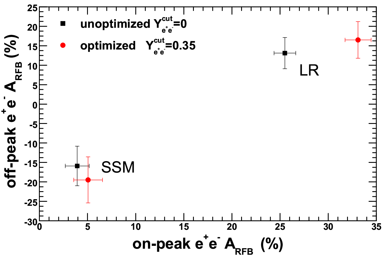
In Fig. 6 we show the different asymmetries for both LR model and the SSM. Central values are calculated in both optimized and un-optimized cases. The error bar are estimated according to the formula

Here $N^{F}/N^{B}$ is the forward/backward events, $N^{A}=N^{F}-N^{B}$ is the asymmetric events and $N$ is the total events. The relation between err and significance is $S_{A}=A_{\rm{FB}}/\rm{err}$, where $S_{A}$ is the significance with reconstruction efficiency. In our estimation, the $b\bar{b}$ and $t\bar{t}$ reconstruction efficiencies are taken as $\epsilon_{b\bar{b}}=0.36$ and $\epsilon_{t\bar{t}}=0.075$ respectively [8]. For the $b\bar{b}$ and $t\bar{t}$ final states, next-to-leading order QCD contribution to the asymmetric cross sections are included. For the $b\bar{b}$ final state, QCD NLO contribution to on-peak $A_{\rm{RFB}}$ is 1.38% for the optimized case and 0.96% for the un-optimized $Y^{\rm{f\bar{f}}}_{\rm{cut}}=0$ case. The contribution is a little bit larger than the statistic error (see the left-bottom diagram of Fig. 6), so this effect should be taken into account. For the $t\bar{t}$ final states, QCD NLO contribution to on-peak $A_{\rm{E}}$ is 0.53% for the optimized case, which is much less than the statistic error (see the right-bottom diagram of Fig. 6), so this effect can be neglected.

From the Fig. 6, the two models give the apparently different predictions for two asymmetries. Even without optimal cuts, the asymmetries can be utilized to discriminate models in this case. However in the real case, the asymmetry difference for various models might be small. In this case the optimal cuts can help to improve the capacity to discriminate models. From the figure it is obviously that the central values of the asymmetries separate more apart in both the LR model and the SSM. However, due to the decreasing of the statistics, the error bar becomes a little bit larger for the optimized case.

References

- [1] P. Langacker, R. W. Robinett, and J. L. Rosner, Phys. Rev. D 30, 1470 (1984).
- [2] M. Cvetic and S. Godfrey, (1995), arXiv: hep-ph/9504216.
- [3] M. Dittmar, Phys. Rev. D 55, 161 (1997).
- [4] M. Dittmar, A.-S. Nicollerat, and A. Djouadi, Phys. Lett. B583, 111 (2004), arXiv: hep-ph/0307020.
- [5] S. Godfrey and T. A. W. Martin, Phys. Rev. Lett. 101, 151803 (2008).
- [6] F. Petriello and S. Quackenbush, Phys. Rev. D 77, 115004 (2008).
- [7] P. Langacker, Rev. Mod. Phys. 81, 1199 (2009).
- [8] R. Diener, S. Godfrey, and T. A. W. Martin, (2009), arXiv: 0910.1334.
- [9] R. Diener, S. Godfrey, and T. A. W. Martin, Phys. Rev. D 80, 075014 (2009).
- [10] R. Diener, S. Godfrey, and T. A. W. Martin, (2010), arXiv: 1006.2845.
- [11] V. Barger and K. Whisnant, Phys. Rev. D 36, 979 (1987).
- [12] F. del Aguila, M. Quiros, and F. Zwirner, Nucl. Phys. B287, 419 (1987).
- [13] V. Barger, N. G. Deshpande, J. L. Rosner, and K. Whisnant, Phys. Rev. D 35, 2893 (1987).
- [14] U. Baur and K. H. Schwarzer, Phys. Lett. B180, 163 (1986).
- [15] S. Godfrey, J. L. Hewett, and T. G. Rizzo, Phys. Rev. D 37, 643 (1988).
- [16] J. L. Rosner, Phys. Lett. B221, 85 (1989).
- [17] F. Boudjema, F. M. Renard, and C. Verzegnassi, Phys. Lett. B202, 411 (1988).
- [18] J. D. Anderson, M. H. Austern, and R. N. Cahn, Phys. Rev. D 46, 290 (1992).
- [19] M. Cvetic and P. Langacker, Phys. Rev. D46, 14 (1992).
- [20] P. Langacker and M. Luo, Phys. Rev. D 45, 278 (1992).
- [21] F. Feruglio, Presented at 26th Rencontres de Moriond, Les Arcs, France, Mar 10-17, 1991.
- [22] C. Verzegnassi, Invited Seminar at Beyond the Standard Model, Int. Europhysics Conf. on High Energy Physics, Uppsala, Sweden, Jun 25 - Jul 1, 1987.
- [23] J. L. Rosner, In Proc. of 1986 Summer Study on the Physics of Superconducting Super Collider, Snowmass, CO, Jun 23 - Jul 11, 1986.
- [24] J. L. Rosner, Phys. Rev. D 54, 1078 (1996).
- [25] F. del Aguila, M. Cvetič, and P. Langacker, Phys. Rev. D 48, R969 (1993).
- [26] DELPHI, J. Abdallah et al., Eur. Phys. J. C45, 589 (2006), arXiv: hep-ex/0512012.
- [27] P. Langacker, (2009), arXiv: 0911.4294.
- [28] S. Gopalakrishna, T. Han, I. Lewis, Z.-g. Si, and Y.-F. Zhou, Phys. Rev. D 82, 115020 (2010).
- [29] J. H. Kühn and G. Rodrigo, Phys. Rev. Lett. 81, 49 (1998).
- [30] J. H. Kühn and G. Rodrigo, Phys. Rev. D 59, 054017 (1999).
- [31] O. Antuñano, J. H. Kühn, and G. Rodrigo, Phys. Rev. D 77, 014003 (2008).
- [32] P. Ferrario and G. Rodrigo, Phys. Rev. D 78, 094018 (2008).
- [33] Y.-k. Wang, B. Xiao, and S.-h. Zhu, Phys. Rev. D 82, 094011 (2010).
- [34] Y.-k. Wang, B. Xiao, and S.-h. Zhu, (2010), Phys. Rev. D 83, 015002 (2011).
- [35] B. Xiao, Y.-K. Wang, Z.-Q. Zhou, and S.-h. Zhu, (2011), arXiv: 1101.2507.
- [36] The CDF, T. Aaltonen et al., (2011), 1101.0034.