Solar cycle variations of large frequency separations of acoustic modes: Implications for asteroseismology
Abstract
We have studied solar cycle changes in the large frequency separations that can be observed in Birmingham Solar Oscillations Network (BiSON) data. The large frequency separation is often one of the first outputs from asteroseismic studies because it can help constrain stellar properties like mass and radius. We have used three methods for estimating the large separations: use of individual p-mode frequencies, computation of the autocorrelation of frequency-power spectra, and computation of the power spectrum of the power spectrum. The values of the large separations obtained by the different methods are offset from each other and have differing sensitivities to the realization noise. A simple model was used to predict solar cycle variations in the large separations, indicating that the variations are due to the well-known solar cycle changes to mode frequency. However, this model is only valid over a restricted frequency range. We discuss the implications of these results for asteroseismology.
Keywords:
methods: data analysis, Sun: helioseismology, Sun: oscillations1 Introduction
Helioseismic and asteroseismic frequency-power spectra contain a rich array of oscillation peaks. The separation in frequency between acoustic (p) modes with the same harmonic degree () and consecutive radial orders () is known as the large frequency separation, . Insights into stellar structure and evolution can be obtained by determining because it can help constrain stellar properties, such as mass, radius, and log , with high precision (Kallinger et al., 2009; Stello et al., 2008; Stello et al., 2009a; Miglio et al., 2009, e.g.). Therefore, one of the first aims when analysing any new set of asteroseismic data of a solar-type star is to determine the of the observable low- modes.
The frequencies of high order p modes are expected to follow approximately the asymptotic relation (Tassoul, 1980) and so may be regarded as approximately constant. However, is dependent on both frequency and and the often quoted in literature is that observed for modes.
In this paper we describe three methods of determining the large separation (see Section 2). The most intuitive way of determining is to use the individual mode frequencies (see Section 2.1). However, sometimes the signal-to-noise ratio of the oscillations is insufficient to allow the robust extraction of individual oscillation frequencies. This can be the case for asteroseismic data and can be true for solar data, for example, when the duty cycle is low. It is therefore convenient to be able to obtain without determining the individual mode frequencies and so we also obtain using the autocorrelation of frequency-power spectra (Section 2.2) and using the power spectrum of the power spectrum (Section 2.3).
It is well known that the Sun’s p-mode frequencies vary throughout the 11-yr solar activity cycle with frequencies being at their largest when solar activity is at its maximum (Woodard & Noyes, 1985; Pallé et al., 1989; Elsworth et al., 1990; Jiménez-Reyes et al., 2003; Chaplin et al., 2007; Jiménez-Reyes et al., 2007, e.g.). By examining the changes in the observed p-mode frequencies throughout the solar cycle, we can learn about solar-cycle-related processes that occur beneath the Sun’s surface. In Section 3 we show that solar cycle variations in can be observed in Birmingham Solar Oscillations Network (BiSON) data. This could have important consequences for asteroseismic studies, which use to determine fundamental stellar properties. We also show that a simple model can be used to predict the observed variation in (Section 3.1).
In Section 4 we discuss the impact of observational choices on the obtained . For example, Kholikov & Hill (2008) determine the solar using GONG and MDI data and some intriguing differences are found between their results and the obtained here. A discussion of the implications of our results, for both astero- and helioseismology, is provided in Section 5.
2 Determining the large separations
BiSON has now been collecting data for over 30 yr. The quality of the early data, however, is poor compared to more recent data because of poor time coverage. Here, we have analyzed the mode frequencies observed by BiSON during the last solar cycle i.e. from 1996 April 11 to 2010 October 8. The precision with which p-mode frequencies can be determined is directly related to the length of time series under consideration. Consequently, p-mode frequencies are often determined from time series whose lengths are of the order of years. However, a compromise must be made here regarding the appropriate length of time series for study so that changes during the solar cycle can be resolved. The observations made by BiSON were divided into 182.5-d-long independent subsets. Over the total observation period the fractional duty cycles, or “fills”, of the 182.5-d subsets ranged from 0.72 to 0.88.
Each method of determining the large separation must be applied over a certain range in frequency. Initially we considered the range µHz. At frequencies lower than µHz there is very little change in frequency over the course of the solar cycle and so it is reasonable to assume that the large separation is also relatively constant. Above µHz the relationship between frequency shift and activity changes, as the magnitude of the solar cycle frequency shift decreases (Libbrecht & Woodard, 1990; Chaplin et al., 1998). Furthermore, above µHz it appears that modes experience a decrease in frequency as activity increases (Ronan et al., 1994; Chaplin et al., 1998). Kholikov & Hill use the range µHz and so in Section 4 we have repeated our analysis over this frequency range. We now describe in turn each of the three methods of determining .
2.1 The fitted method
The large separations can be obtained from the individual mode frequencies, . Estimates of the mode frequencies were extracted from each 182.5-d subset by fitting a modified Lorentzian model to the data using a standard likelihood maximization method (Fletcher et al., 2009). The large separations are then given by
| (1) |
However, determination of the average using the individual mode frequencies is complicated by the fact that is correlated to . Therefore a linear function was fitted between and mode frequency, , and the gradient of this linear fit giving the average large frequency separation, . The linear fit was weighted by the formal errors associated with the fitted frequencies. The fit was performed separately for each and the mean of the gradients was determined. The left-hand panel of Fig. 1 shows that a linear fit represents the data well. For the remainder of this paper we refer to this method of determining the large separations as the “fitted method”. Although modes with as high as 5 can be observed in Sun-as-a-star data these modes are unlikely to contribute significantly to the observed results as their amplitudes are significantly smaller than modes with . Therefore, when using the individual mode frequencies to determine we have used information from modes with only. We have estimated the average for all and we have examined for each individually.


Monte Carlo simulations were used to determine whether the uncertainties returned by the linear fit reflect the true uncertainties associated with this method of determining the large separation. 400 artificial BiSON-like 182.5-d time series were generated (Chaplin et al., 2006). The mode frequencies used to generate the data were shifted in the manner expected due to the solar cycle (see Broomhall et al., 2009a, and Section 3.1 of this paper). Although the magnitude of the shift placed on each individual mode was dependent on mode frequency and , the size of the frequency shifts were based on an mode at µHz being shifted by µHz. Simulations were also run using a smaller frequency shift but the results were found to be relatively insensitive to the size of the input shift. The ratio of the standard deviation of obtained from the simulations and the mean uncertainty on indicates by how much the observed uncertainties need to be scaled to reflect the true errors. The scaling factors were dependent on both the frequency range used to determine and which were used. The simulated data were given various BiSON-like window functions whose fills represented the range of fills observed here i.e. 0.72-0.88. Although dependent on fill, over the range the scaling factors were approximately constant. Therefore the scaling factor used to determine the size of the errors was an average of the scaling factors obtained for the different simulated fills. When calculating over µHz and using the scaling factor was 1.5 i.e. the true uncertainties associated with the fitted method were 1.5 times larger than the uncertainties implied by the fit.
2.2 The autocorrelation method
In the past cross-correlations of frequency-power spectra were used to estimate the mean shifts in the frequencies of solar p modes. This approach is particularly advantageous when the data have a low S/N, which makes individual mode fitting difficult, because all of the frequency data in the range under consideration are used (Regulo et al., 1994). This method is also applied in asteroseismic studies. For example, Campante et al. (2010) describe an automated method of fitting the autocovariance of frequency-power spectra of asteroseismic data in order to obtain, amongst other parameters, the large frequency separation.
For different frequency lags, , the autocorrelation of a frequency-power spectrum was determined over a given frequency range. Let be the frequency-power spectrum, the lower bound of the frequency range under consideration (i.e. µHz) and the upper limit on the frequency range (i.e. µHz). The autocorrelation, , is then given by
| (2) |
When cross-correlations were first used to determine solar-cycle frequency shifts a second-order polynomial was fitted to the log of the cross-correlation function over µHz around a lag of µHz (Regulo et al., 1994; Jimenez-Reyes et al., 1998). However, Jiménez-Reyes et al. (2001) showed that more accurate results could be obtained by fitting symmetric Lorentzians to the main peak and peaks at the diurnal frequencies over a range of µHz. This approach was based on the assumption that the mode peaks themselves are Lorentzian in shape but neglects mode asymmetries. Fitting the main peak and the diurnal sidebands works well when the duty cycle of the data is low. However, as the fill increases the amplitude of the sidebands decreases and other features become visible in the cross-correlation spectrum. Chaplin et al. (2007) fitted a function based on 7 Lorentzians: 1 for the central peak, 2 for the diurnal frequencies, and 2 each for the and overlapping pairs.
A structure containing the same combination of Lorentzian peaks is observed in the autocorrelation at multiples of the large separation (see, for example, the middle panel of Fig. 1) and so by fitting the autocorrelation function of the frequency-power spectrum centred on a lag of µHz we can determine the average large separation, . We have fitted the peaks on both the positive and negative sides of zero lag and then taken the average of the fitted results. The fitted function, took the form
| (3) |
where was the amplitude of the central peak, was the height of the peak relative to the central peak, was the width of the central peak, was the increase in width of the and overlapping peaks, was the frequency spacing between the central peak and the outer peaks and was a background term. Here represented the central peak, represented the overlap, represented the diurnal sidebands and represented the overlap. The relative height, was fixed at unity for i.e. for the central peak. The increase in width, was fixed at µHz when and 2 i.e. for the central peak and the diurnal sidebands. Finally was fixed at µHz.
Following Chaplin et al. (2007) we assumed that the widths of the diurnal sidebands were the same as the central peak and fixed their frequencies at µHz. The Lorentzians for the overlapping pairs have widths that are wider than the central peak because of the influence of different components of a multiplet. For example an mode, which has one component only, will overlap with the 3 visible (in Sun-as-a-star data) components of an mode at 3 different frequencies. The distances of the overlapping and pairs from the central peak are known as the small separations, . We have used initial guess values for the pair of µHz and for the pair of µHz, based on the average observed spacings over the frequency range of interest. For the remainder of this paper we refer to this method of determining the large separations as the “autocorrelation method”.
The underlying profile of a mode in a frequency-power spectrum is an asymmetric Lorentzian. Two important parameters in characterizing each mode Lorentzian are the height and width. We then define the power of the mode as the total area under the Lorentzian. The autocorrelation function is most influenced by the modes with the largest heights i.e. those modes around µHz. In effect the obtained frequency separation represents a weighted average over the frequency range of interest.
Although the statistics of a frequency-power spectrum is not Gaussian the autocorrelation function is the sum of many points and so the central limit theorem can be applied. Therefore, a standard least squares fitting can be performed. However, the points in the autocorrelation are highly correlated and, although this does not bias the fitted parameters, the formal Hessian uncertainties are an underestimate of the true uncertainties. Monte Carlo simulations, similar to those described in Section 2.1, were performed to estimate a scaling factor by which the Hessian uncertainties needed to be multiplied to better represent the true errors of the fit. The scaling factor showed no systematic dependence on fill over the range examined here. We therefore took the scaling factor to be the mean of the simulated scaling factors. When calculating the autocorrelation function over the scaling factor was 3.5.
The middle panel of Fig. 1 shows an example of the autocorrelation. A prominent peak is observed and the model provides a good fit to the data. The fill of the plotted data is relatively high for ground-based observations (0.88) and so overlaps between the and modes are clearly visible, whereas the daily harmonic peaks are suppressed.
2.3 The PSPS method
An alternative way of determining the large separations that is frequently employed in asteroseismic studies (Roxburgh & Vorontsov, 2006; Roxburgh, 2009; Mosser & Appourchaux, 2009; Hekker et al., 2010; Mathur et al., 2010; Mosser & Appourchaux, 2010, e.g.) is to calculate the power spectrum of the power spectrum (). A significant peak is observed in the power spectrum of the power spectrum at half the large separation. This method is equivalent to determining the autocorrelation of the time series. Kholikov & Hill (2008) used the autocorrelation of time series to determine the acoustic radius, , which is related to the large separation, , by the following equation:
| (4) |
The was determined, over the frequency range of interest. We have oversampled the data by a factor of 10 and this was done by adding zeroes to the end of the frequency range of interest. A peak is clearly visible at half the large separation (see the right-hand panel of Fig. 1). A Gaussian was fitted to this peak to determine the value of half the separation. Two alternate ways of finding the central frequency of the peak are by interpolation and by determining the centroid of the peak. However, these methods were found to be more sensitive to the background noise and so we have instead used the results obtained by fitting a Gaussian. For the remainder of this paper we refer to this method of determining as the “power spectrum of the power spectrum (PSPS) method”.
To determine whether the uncertainties from fitting a Gaussian to the peak are representative of the true uncertainties Monte Carlo simulations were performed that were similar to those described in Section 2.1. The simulations showed that the uncertainties were underestimated by a factor that was dependent on the frequency range under consideration. Different BiSON-like window functions were applied to the simulated time series. As with the other two methods the scaling factor was independent of the fill over the range of fills observed here. When calculating the over the scaling factor was 1.8.
3 Solar cycle variations in

Fig. 2 shows the large separations obtained from the 182.5-d data sets using the fitted, autocorrelation, and PSPS methods. For the fitted method the mean for modes with was obtained. As we have used Sun-as-a-star data the autocorrelation and PSPS methods contain information from all visible . However, in practice, modes with will dominate as they are most prominent. Solar cycle variations are clearly visible in the fitted and autocorrelation method results. The PSPS method results are noisier and so it is difficult to see any solar cycle variations.
There is an offset between the large separations obtained by the three methods (also see the top panel of Fig. 3). The difference between the fitted and autocorrelation methods can be explained in terms of the different frequency dependence of the methods combined with the frequency dependence of the large separations themselves. The autocorrelation method is heavily weighted towards the most prominent modes. However, the fitted method will be weighted towards lower-frequency modes since the frequencies of these modes can be obtained more precisely than high-frequency modes (because they have longer damping times and consequently narrower widths in frequency-power spectra). Weighting the linear fit between and by a combination of mode height and the errors associated with the frequencies reduces the disparity but only very marginally. The PSPS method is weighted by the power (and not the height) of the modes. Mode power drops off less rapidly with frequency than mode height and so the PSPS method is weighted towards higher-frequency modes than the other two methods. Since increases with frequency over the range of frequencies considered here, the determined by the PSPS method is larger than the obtained by the other methods.

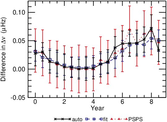
The large separations have also been obtained from two sets of data that were simulated for the solar Fitting at Low Angular Degree Group (FLAG) (Chaplin et al., 2006, top panel of Fig. 3). The data were simulated in the time domain. In the first simulated data set (FLAG1) the properties of the oscillations were constant but in the second data set (FLAG2) the oscillation properties were modulated by the solar cycle. For the fitted method the mean for modes with was obtained while the autocorrelation and PSPS methods contain information from all visible . The large separations determined by the autocorrelation and PSPS methods vary significantly more than the large separations determined using the fitted method. This indicates that the autocorrelation and PSPS methods are more sensitive to the realisation noise.
The bottom panel of Fig. 3 shows the difference between the large separations obtained in the FLAG2 data set and the large separations obtained from the FLAG1 data set. This difference uncovers the simulated solar cycle effect, which alters the large separations by about µHz. It should be remembered that this data set is only yr in length and so does not quite cover an entire solar cycle.
3.1 Predicting variations in the large separations using solar cycle frequency correction techniques
Broomhall et al. (2009a) corrected Sun-as-a-star p-mode frequencies for the effect of the solar cycle. Here, we have reversed the procedure applied to implement these corrections in order to predict the frequencies of p modes in Sun-as-a-star data at a particular level of activity. We have used the frequencies quoted in table 3 of Broomhall et al. (2009b) as a reference set of frequencies. These frequencies were determined by fitting 23 yr of BiSON data using the methods described in Fletcher et al. (2009). The raw fitted frequencies were then corrected, using the methods described in Broomhall et al. (2009a), to give the frequencies that would have been observed at the canonical quiet Sun activity level, and it is these frequencies that we use here. The correction performed by Broomhall et al. (2009a) comes in three parts: a linear solar cycle correction, a “devil-in-the-detail” correction, and a Sun-as-a-star correction.
The linear solar cycle correction is well known and can be used to correct mode frequencies to a nominal activity level. The correction is based on the assumption that variations in global activity indices can be used as proxies for low- frequency shifts. It is also assumed that the correction can be parameterised as a linear function of the chosen activity measure. Here we have used the 10.7-cm flux (Tapping & Detracey, 1990) for which these assumptions are robust at the level of precision of the data (Broomhall et al., 2009a, and references therein). The canonical quiet-Sun value of the radio flux is fixed from historical observations at . The size of the linear correction is also dependent on mode frequency and . Here we have used the frequency dependence derived by Chaplin et al. (2001); Chaplin et al. (2004). The dependence is small for but is included nonetheless and occurs because of differences in the mode inertia (Christensen-Dalsgaard & Berthomieu, 1991).
The “devil-in-the-detail” correction accounts for cross-talk between the variations of different mode parameters over the solar cycle, and the distribution of activity levels over the period of observations. As we are using relatively short time series here, this effect will be negligible and so this correction was not performed.
The Sun-as-a-star correction accounts for the fact that when using Sun-as-a-star observations the rotationally split components of a mode have different visibilities. As the plane of the Sun’s rotation axis is nearly perpendicular to the line-of-sight, only modes where is even have significant visibility. Furthermore, estimates of the centroid frequencies are dominated by the components, as they are most prominent. The difference between the centroid and fitted frequencies depends on the level of activity over the period the observations were made. When the solar activity is at a minimum the components are observed to be in a near-symmetrical arrangement and so the fitted centroid is close to the true centroid frequency. However, at moderate to high activity levels this is not the case as the mode components are not arranged symmetrically. For example, the components of an mode will experience a larger shift at high activities than the component. The magnitude of the observed asymmetry is related to the inhomogeneous distribution of the magnetic activity over the solar surface and the spherical harmonic associated with each visible component. Therefore, the fitted frequencies differ from the true centroids by an amount that is dependent on . Appourchaux & Chaplin (2007) describe how to make a Sun-as-a-star correction, which is determined using the so-called coefficients that are found from fits for an unresolved Sun.

Once the frequencies for a particular time series at a known activity level have been predicted we can use these frequencies to determine the average large frequency separation using the fitted method. The predicted large separations are plotted in Fig. 4 along with the observed determined by the three methods. For the fitted method the mean for modes with was obtained, while the autocorrelation and PSPS methods contain information from all modes visible in Sun-as-a-star data. The agreement between the predicted large separations and the large separations observed using the fitted method is very good. The good agreement between the predicted and observed large separations implies that the observed variation can be explained in terms of the observed shifts of the individual mode frequencies.
Notice that the observed large separations show more short-term variability than the predicted in the declining phase of cycle 23 and the minimum between cycles 23 and 24. It has long been observed that p-mode frequencies respond to short-term changes in activity (Rhodes et al., 2002, e.g). Furthermore, a similar behaviour was observed in the solar-cycle frequency shifts by Broomhall et al. (2009b) and Fletcher et al. (2010). Fig. 2 shows that the quasi-biennial variations observed in the large separations are in agreement with those observed in the frequency shifts by Broomhall et al. and Fletcher et al.. This implies that the shorter-term variations show some frequency dependence. However, the amplitude of the shorter-term variations in is smaller than the amplitude of the 11-yr variation, indicating that the frequency dependence of the shorter-term variation is weaker than the frequency dependence of the 11-yr cycle. This is in agreement with the results of Fletcher et al. (2010).

Fig. 5 shows a direct comparison between the model and fitted method observed using modes with . Although not shown here a similar analysis was performed for the autocorrelation and PSPS methods. Linear fits between the modelled and observed were performed and the gradients of the linear fits were within of unity for all three methods. This suggests that the magnitude of the solar cycle effect is the same for each method of deriving and that all three methods produce variations in that are in agreement with the model, even if the absolute values of differ (e.g. Fig. 4).
3.2 The dependence of the solar cycle variations in the large separations

As we are using Sun-as-a-star data the large separations cannot be determined for each separately using the autocorrelation and PSPS methods. However, the fitted method can be used to examine the dependence of the variation in . Fig. 6 shows the solar cycle variations in the large separations for individual . There is an offset between the different large separations observed in the different , demonstrating the dependence of the large separations. increases with increasing because the depth of the cavity in which the modes are trapped decreases and so the acoustic radius, which is inversely proportional to , also decreases with increasing .
The individual- large separations are generally well reproduced by the model described in Section 3.1. Figs 6 and 7 show that the magnitude of the observed 11-yr cycle variations increase slightly with . For the model values the peak-to-trough variation is µHz, whereas the variation is µHz and the variation is µHz. Solar cycle shifts in mode frequencies are dependent on because the size of the perturbation is inversely related to the mode inertia, which decreases with increasing (Libbrecht & Woodard, 1990, e.g.). However, this effect is negligible over the range of considered here (). As mentioned in Section 3.1 there is an dependence in the solar cycle frequency shifts that occurs because magnetic activity is inhomogenously spread across the solar surface. It is this dependence that causes the differences with in the amplitudes of the solar cycle variations in .


Fig. 7 shows a direct comparison between the model and observed of each . The model has been computed separately for each . Although offset from each other the ranges of the axes are the same and so it is again possible to see that the modes show more variation throughout the solar cycle than the , and, in particular, the modes. Linear fits between the modelled and observed were again performed and the gradients of the linear fits lie within of unity for all three , with the modes showing the best agreement.
4 Impact of observational choices
Kholikov & Hill (2008) observed solar cycle variations in the acoustic radius, which is inversely proportional to , in Global Oscillations Network Group (GONG) and Michelson Doppler Imager (MDI) data. To allow a comparison with the results of Kholikov & Hill (2008) we have repeated the above analysis using the same frequency range i.e. µHz. Kholikov & Hill determine the acoustic radius for individual . Therefore we have compared the Kholikov & Hill results with the found here. Before that we first discuss the impact of changing the frequency range on the -averaged results.
Fig. 8 shows the large separations found using the autocorrelation, fitted, and PSPS methods, and the model predictions. The fitted method was used to determine the average for modes with . The change in frequency range has increased the offset between the results of the three methods. Changing the frequency range has had very little effect on the determined using the autocorrelation method because the autocorrelation method is weighted most heavily towards the most prominent modes, at µHz. However, the fitted method large separations have been shifted downwards by approximately µHz and the short term structure of the large separations has changed. The shift in the fitted method large separations arises because the obtained are weighted towards the lowest frequency modes in the range under consideration and modes at µHz have a lower than modes at µHz. The change in the short-term structure of the fitted method large separations could be due to extra noise, which is introduced into the results by including the higher frequency modes, whose frequencies cannot be determined precisely because of short mode lifetimes. It could also be because low-frequency modes are more sensitive to realization noise, due to long mode lifetimes. Another possibility is that the changes in the short-term structure could reflect the frequency dependence of the shorter-term signal.
The large separations determined by the PSPS method have been shifted upwards by approximately µHz. As mentioned earlier the PSPS method is weighted by mode power and the power of modes in the range µHz is, on average, higher than the power of modes in the range µHz. Since modes in the frequency range µHz have larger than lower-frequency modes the large separations determined by the PSPS method are increased.

Also plotted in Fig. 8 are the modelled determined over the frequency range µHz and for modes with . As expected they maintain approximate agreement with the fitted method results (as opposed to the autocorrelation and PSPS results). However, the agreement between the modelled and fitted is clearly not as good over this frequency range as was found in Fig. 6 (over µHz).

Fig. 9 shows a direct comparison between the model and fitted method observed for µHz and . Once again, although not plotted here a similar analysis was performed for the autocorrelation and PSPS methods. The gradients of the linear fits all show departures from unity: the gradient of the fitted method is from unity, the autocorrelation is from unity, and the PSPS method is from unity. The observed show more variation than was predicted by the model.
Further investigation reveals that this is because the lower limit of the frequency range has been changed from µHz to µHz, which implies that the frequency dependence of the solar cycle perturbation on mode frequencies does not reflect the perturbation observed in BiSON data at low frequencies.

Fig. 10 shows the -dependence of the large separations using the frequency range µHz. Comparison with Fig. 6 shows that the large separations are less sensitive to the change in frequency range than the and modes. Notice that the models do not represent the observed large separations as well over this frequency range.


Fig. 11 shows a direct comparison between the model and observed for each . Although the gradient of the linear fit to the mode results lies within of unity the gradients of the fits to the and modes differ significantly from unity: for and for . Again the observed show more variation than was predicted by the model. Therefore, the model does not represent the data for and modes over this frequency range.
Kholikov & Hill (2008) use the autocorrelation of time series to obtain the acoustic radius. This method is analogous to the PSPS method used here. Kholikov & Hill use resolved Sun GONG and MDI data and so are able to isolate individual . Here, since we are using Sun-as-a-star data we can only determine for individual using the fitted method. Therefore, in the left-hand panel of Fig. 11 we compare the results of Kholikov & Hill (2008) with the determined using the fitted method. Kholikov & Hill determined the offset for 36 d (GONG) and 72 d (MDI) time series. To allow a comparison with the results derived here we have plotted the weighted mean of the results of Kholikov & Hill over 5 and 3 points respectively, where the weights were given by the errors of the observations. The range of observed in the BiSON data is significantly larger than is observed by Kholikov & Hill. A linear fit between the results of Kholikov & Hill and the model was performed. The gradients of both fits were significantly shallower than unity: away from unity for the GONG results and for the MDI results. It should be noted that the uncertainties associated with the results of Kholikov & Hill were very small. While, to the eye, the gradients of the slopes look similar to unity, relative to the size of the uncertainties, the departures from unity are significant.
The GONG and MDI found by Kholikov & Hill are offset from the BiSON results obtained here and from each other. This suggests that not only do different methods of determining result in different values (see e.g. Fig. 9) but that also different data result in different values of . Kholikov & Hill were unable to explain this offset. The autocorrelation method was used to determine for 182.5-d sets of data observed by the Global Oscillations at Low Frequencies (Gabriel et al., 1995; Jiménez-Reyes et al., 2003; García et al., 2005, GOLF;) instrument onboard the SOlar and Heliospheric Observatory (SOHO) spacecraft. GOLF has been collecting data since 1996 and so we have been able to analyze data covering almost the entirety of solar-cycle 23, i.e., from 1996 April 11 to 2009 April 7. Although not shown here the BiSON and GOLF results were in very good agreement and the differences between the BiSON and GOLF were, on average, significantly smaller than the associated error bars. It is possible, therefore, that the main offset between the BiSON and the observed by Kholikov & Hill occurs because of the different methodologies employed.
5 Summary and Discussion
The three different methods resulted in different values of . The results of Kholikov & Hill (2008) were offset from each other and from the BiSON data. The different values for the different methods can be understood in terms of the weighting with frequency of the methods and the frequency dependence of . However, this does not explain the difference between the two sets of Kholikov & Hill results
The observed offsets could be important for asteroseismic studies, which use the determined to infer stellar properties such as radius and mass. Stello et al. (2009b) showed that the following scaling relation holds over most of the HR diagram and results in errors that are probably below 1 per cent,
| (5) |
where is the mass of a star, is the radius of as star and denotes the values for the Sun. The farthest separated like-for-like values considered here are the fitted method and PSPS method results for the frequency range µHz, which are on average separated by µHz. If we take the fitted method results to represent those of the Sun and the PSPS method results to represent those of another star and assume that the , equation 5 implies that the “other” star is 0.3 per cent larger than the Sun, which is within the errors implied by Stello et al. (2009b).
The fitting method appears to be the cleanest way of determining as it is less sensitive to the noise realization than the other two methods. However, it is not always possible to determine the frequencies of the individual modes because of poor signal-to-noise levels and poor fill. If this is the case, for the data examined here, the autocorrelation method produced more stable results than the PSPS method.
Solar cycle changes in were visible in the results of the fitted and autocorrelation methods. This again suggests that care is needed in using in determining properties of stars. The amplitude of the solar cycle effect is smaller than µHz (see Fig. 2) and, therefore, using the same logic as above, the solar cycle variations in the Sun would result in changes in stellar radii that are within error estimates. However, the Sun is a relatively quiet star and so it is possible that would vary more in other stars, resulting in systematic errors in estimated masses and radii.
We have shown that the observed solar cycle changes in can be predicted using a simple model, which is valid over the frequency range µHz. This implies that the changes in are due to the frequency dependence of the solar cycle changes in . The correlation with the model is less good over the frequency range µHz. This is mainly because the model underestimates the size of the perturbation in at low frequencies, suggesting that the BiSON data do not follow the assumed frequency dependence at low frequencies. This could be because the assumed frequency dependence was derived using intermediate- and high-degree GONG data and not (low-) BiSON data (Chaplin et al., 2001; Chaplin et al., 2004). The model also breaks down to different extents for the different . This could be because the inertia scaling is not correct for the BiSON data at low frequencies.
Recently García et al. (2010) observed signatures of a stellar activity cycle in asteroseismic data obtained by the Convection Rotation and Planetary Transits (Michel et al., 2008, CoRoT; e.g.) space mission. With the prospect of longer asteroseismic data sets () becoming available through, for example, Kepler (Chaplin et al., 2010; Koch et al., 2010) there will be opportunities to observe activity cycles in other stars. These observations will provide constraints for models of stellar dynamos under conditions different from those in the Sun.
Acknowledgements
The authors thank S. Kholikov for providing the results of their paper: Kholikov & Hill (2008). This paper utilizes data collected by the Birmingham Solar-Oscillations Network (BiSON). We thank the members of the BiSON team, both past and present, for their technical and analytical support. We also thank P. Whitelock and P. Fourie at SAAO, the Carnegie Institution of Washington, the Australia Telescope National Facility (CSIRO), E.J. Rhodes (Mt. Wilson, Californa) and members (past and present) of the IAC, Tenderize. BiSON is funded by the Science and Technology Facilities Council (STFC). The authors also acknowledge the financial support of STFC.
References
- Appourchaux & Chaplin (2007) Appourchaux T., Chaplin W. J., 2007, A&A, 469, 1151
- Broomhall et al. (2009a) Broomhall A., et al., 2009a, A&A, 503, 241
- Broomhall et al. (2009b) Broomhall A., et al., 2009b, MNRAS, 396, L100
- Campante et al. (2010) Campante T. L., Karoff C., Chaplin W. J., Elsworth Y. P., Handberg R., Hekker S., 2010, MNRAS, 408, 542
- Chaplin et al. (2001) Chaplin W. J., Appourchaux T., Elsworth Y., Isaak G. R., New R., 2001, MNRAS, 324, 910
- Chaplin et al. (1998) Chaplin W. J., Elsworth Y., Isaak G. R., Lines R., McLeod C. P., Miller B. A., New R., 1998, MNRAS, 300, 1077
- Chaplin et al. (2004) Chaplin W. J., Elsworth Y., Isaak G. R., Miller B. A., New R., 2004, MNRAS, 352, 1102
- Chaplin et al. (2007) Chaplin W. J., Elsworth Y., Miller B. A., Verner G. A., New R., 2007, ApJ, 659, 1749
- Chaplin et al. (2006) Chaplin W. J., et al., 2006, MNRAS, 369, 985
- Chaplin et al. (2010) Chaplin W. J., et al., 2010, ApJL, 713, L169
- Christensen-Dalsgaard & Berthomieu (1991) Christensen-Dalsgaard J., Berthomieu G., 1991, Theory of solar oscillations. pp 401–478
- Elsworth et al. (1990) Elsworth Y., Howe R., Isaak G. R., McLeod C. P., New R., 1990, Nature, 345, 322
- Fletcher et al. (2010) Fletcher S. T., Broomhall A., Salabert D., Basu S., Chaplin W. J., Elsworth Y., García R. A., New R., 2010, ApJL, 718, L19
- Fletcher et al. (2009) Fletcher S. T., Chaplin W. J., Elsworth Y., New R., 2009, ApJ, 694, 144
- Gabriel et al. (1995) Gabriel A. H., et al., 1995, Sol. Phys., 162, 61
- García et al. (2010) García R. A., Mathur S., Salabert D., Ballot J., Régulo C., Metcalfe T. S., Baglin A., 2010, Science, 329, 1032
- García et al. (2005) García R. A., Turck-Chièze S., Boumier P., Robillot J. M., Bertello L., Charra J., Dzitko H., Gabriel A. H., Jiménez-Reyes S. J., Pallé P. L., Renaud C., Roca Cortés T., Ulrich R. K., 2005, A&A, 442, 385
- Hekker et al. (2010) Hekker S., Broomhall A., Chaplin W. J., Elsworth Y. P., Fletcher S. T., New R., Arentoft T., Quirion P., Kjeldsen H., 2010, MNRAS, 402, 2049
- Jiménez-Reyes et al. (2007) Jiménez-Reyes S. J., Chaplin W. J., Elsworth Y., García R. A., Howe R., Socas-Navarro H., Toutain T., 2007, ApJ, 654, 1135
- Jiménez-Reyes et al. (2001) Jiménez-Reyes S. J., Corbard T., Pallé P. L., Roca Cortés T., Tomczyk S., 2001, A&A, 379, 622
- Jiménez-Reyes et al. (2003) Jiménez-Reyes S. J., García R. A., Jiménez A., Chaplin W. J., 2003, ApJ, 595, 446
- Jimenez-Reyes et al. (1998) Jimenez-Reyes S. J., Regulo C., Palle P. L., Roca Cortes T., 1998, A&A, 329, 1119
- Kallinger et al. (2009) Kallinger T., Weiss W. W., De Ridder J., Hekker S., Barban C., 2009, in B. Soonthornthum, S. Komonjinda, K. S. Cheng, & K. C. Leung ed., Astronomical Society of the Pacific Conference Series Vol. 404 of Astronomical Society of the Pacific Conference Series, Oscillating Red Giants in the CoRoT Exo-field: An Asteroseismic Radius and Mass Determination. pp 307–+
- Kholikov & Hill (2008) Kholikov S., Hill F., 2008, Sol. Phys., 251, 157
- Koch et al. (2010) Koch D. G., et al., 2010, in Bulletin of the American Astronomical Society Vol. 42 of Bulletin of the American Astronomical Society, The Design and On-Orbit Performance of the Kepler Mission. pp 302–+
- Libbrecht & Woodard (1990) Libbrecht K. G., Woodard M. F., 1990, Nature, 345, 779
- Mathur et al. (2010) Mathur S., García R. A., Régulo C., Creevey O. L., Ballot J., Salabert D., Arentoft T., Quirion P., Chaplin W. J., Kjeldsen H., 2010, A&A, 511, A46+
- Michel et al. (2008) Michel E., et al., 2008, Science, 322, 558
- Miglio et al. (2009) Miglio A., Montalbán J., Baudin F., Eggenberger P., Noels A., Hekker S., De Ridder J., Weiss W., Baglin A., 2009, A&A, 503, L21
- Mosser & Appourchaux (2009) Mosser B., Appourchaux T., 2009, A&A, 508, 877
- Mosser & Appourchaux (2010) Mosser B., Appourchaux T., 2010, ArXiv e-prints
- Pallé et al. (1989) Pallé P. L., Régulo C., Roca Cortés T., 1989, A&A, 224, 253
- Regulo et al. (1994) Regulo C., Jimenez A., Palle P. L., Perez Hernandez F., Roca Cortes T., 1994, ApJ, 434, 384
- Rhodes et al. (2002) Rhodes Jr. E. J., Reiter J., Schou J., 2002, in A. Wilson ed., From Solar Min to Max: Half a Solar Cycle with SOHO Vol. 508 of ESA Special Publication (Noordwijk: ESA SP-508), Solar cycle variability of high-frequency and high-degree p-mode oscillation frequencies. pp 37–40
- Ronan et al. (1994) Ronan R. S., Cadora K., Labonte B. J., 1994, Sol. Phys., 150, 389
- Roxburgh (2009) Roxburgh I. W., 2009, A&A, 506, 435
- Roxburgh & Vorontsov (2006) Roxburgh I. W., Vorontsov S. V., 2006, MNRAS, 369, 1491
- Stello et al. (2008) Stello D., Bruntt H., Preston H., Buzasi D., 2008, ApJL, 674, L53
- Stello et al. (2009a) Stello D., et al., 2009a, ApJ, 700, 1589
- Stello et al. (2009b) Stello D., et al., 2009b, MNRAS, 400, L80
- Tapping & Detracey (1990) Tapping K. F., Detracey B., 1990, Sol. Phys., 127, 321
- Tassoul (1980) Tassoul M., 1980, ApJS, 43, 469
- Woodard & Noyes (1985) Woodard M. F., Noyes R. W., 1985, Nature, 318, 449