Homogeneous links and the Seifert matrix
Abstract
Homogeneous links were introduced by Peter Cromwell, who proved that the projection surface of these links, that given by the Seifert algorithm, has minimal genus. Here we provide a different proof, with a geometric rather than combinatorial flavor. To do this, we first show a direct relation between the Seifert matrix and the decomposition into blocks of the Seifert graph. Precisely, we prove that the Seifert matrix can be arranged in a block triangular form, with small boxes in the diagonal corresponding to the blocks of the Seifert graph. Then we prove that the boxes in the diagonal has non-zero determinant, by looking at an explicit matrix of degrees given by the planar structure of the Seifert graph. The paper contains also a complete classification of the homogeneous knots of genus one.
1 Introduction
Throughout this paper, we assume that all links and diagrams are oriented. Let be a spanning surface for an oriented link , and let be a regular neighbourhood. Identify with . The associated Seifert matrix with order is defined by the linking number where the ’s are simple closed oriented curves in whose homology classes form a basis of , and is the lifting of out of , in . Then where and are the genus and the Euler characteristic of respectively, and is the number of components of the link. Homology with coefficients in is assumed along this paper.
Let and be the Conway and Alexander polynomials of , in variables and respectively, as defined in [3]. Since after the substitution , we have that the coefficient of the highest degree term in is equal to and the degree of is , whenever does not vanish. In general , which provides the famous lower bound of the genus and in particular it allows to deduce that is a minimal genus spanning surface for if does not vanish.
Suppose now that the spanning surface has been constructed by applying the Seifert algorithm to a diagram of the link . We briefly summarize the main features of this construction: start with a diagram in the -plane. For each Seifert circle a Seifert disc is built in the plane , if there are exactly Seifert circles that contain ; we say that the height of is and write . This collection of discs lives in the upper half-space and they are stacked in such a way that when viewed from above, the boundary of each disc is visible. To complete the projection surface, insert small twisted rectangles (called bands from now on) at the site of each crossing, choosing the half-twist according to the corresponding crossing. Following Cromwell [3], we call a projection surface.
We can now define a graph contained in as follows: take a vertex in each Seifert disc of and, if two discs are joined by a band, join the corresponding vertices by an edge contained in the band. In addition, we label the edge with the sign of the associated crossing in the diagram . This graph, called the Seifert graph of , is in fact a planar graph. The rank of , as defined in graph theory, is one minus the number of vertices plus the number of edges. Since where is the number of Seifert circles and is the number of crossings of , it follows that .
In general, we can consider the decomposition of the graph into its blocks, which are the maximal connected subgraphs without cut vertices. The part of the projection surface (bands and Seifert discs) that corresponds to a block is a submanifold of and will be denoted by , or simply . The graph is a deformation retract of the surface , taking onto ; in particular taking onto and , an equality which is sometimes taken as a definition. Now, a basis of , hence a basis of , can be obtained by juxtaposing basis of , since the cycles in are precisely the cycles of its blocks ([6], lemma 3.1.1). In particular, the rank of is the sum of the ranks of its blocks.
Let be the Seifert matrix defined by any basis of (hence of ), . Our main result is the following:
Theorem 4. Let be a connected diagram of an oriented link , the corresponding Seifert graph and the decomposition of into blocks. Then there is an order in the set of blocks of for which the Seifert matrix for the projection surface is upper block triangular. More precisely, if is the Seifert matrix that corresponds to any basis of , , there exists a permutation such that the Seifert matrix adopts the following form:
A link is homogeneous if it has a homogeneous diagram, which is a diagram in which all the edges of each block of its Seifert graph have the same sign. Alternating and positive diagrams (links) are homogeneous diagrams (links). The knot is an example of homogeneous link which is neither positive nor alternating. Homogeneous links were introduced in 1989 by Cromwell [4]. In Knot Theory the adjective homogeneous was first applied to a certain class of braids by Stallings [18]. Certainly, the closure of a homogeneous braid is a homogeneous diagram, although there are homogeneous links which cannot be presented as the closure of a homogeneous braid, just as there are alternating links which cannot be presented as the closure of alternating braids. In [4] (see also [3]) Cromwell proved the following basic result on homogeneous links:
Theorem (Cromwell). Let be a connected homogeneous diagram of an oriented homogeneous link and the corresponding Seifert graph. Then the highest degree of is the rank of . Furthermore, let be the decomposition of into blocks and the corresponding Seifert matrices, . Then for all and the leading coefficient of is
where is the sign of the edges in and .
Corollary. A projection surface constructed from a connected homogeneous diagram of an oriented link is a minimal genus spanning surface for the link.
Cromwell’s proof is based on a previous construction of a specific resolving tree for calculating the Conway polynomial ([3], Lemma 7.5.1). This means that no crossing is switched more than once on any path from the root of the tree to one of its leaves. The skein relation is then considered, at both the level of the diagram and the corresponding Seifert graph, having in mind that to obtain terms involving powers of when resolving the resolution tree, a crossing must be smoothed in the diagram , or equivalently, an edge must be deleted from the graph . A direct proof of the corollary has been recent and independently suggested by M. Hirasawa. The proof, outlined in a paper by Tetsuya Abe [1] (see also [17]), is strongly based on a difficult result by Gabai [8], which states that the sum of Murasugi of minimal genus surfaces is a minimal genus surface. Hirasawa applies this result to the portions above defined.
In this paper we give a different proof of Cromwell’s theorem, based on the close relation between the Seifert matrix and the decomposition into blocks of the Seifert graph stated in Theorem 4. The key point is the understanding of how the parts of the projection surface corresponding to the blocks are geometrically positioned among them. We remark that Theorem 4 can be useful even in the case in which the diagram is not homogeneous. A special case was already considered by Melvin and Morton in their work on fibred knots of genus two formed by plumbing Hopf bands [13]. We deal with this topic in Section 2.
Since a homogeneous block of the Seifert graph corresponds to an alternating diagram, it follows that each little box in the diagonal of the Seifert matrix has non-zero determinant, according to the work by K. Murasugi [14] (see also [15]) and independently Crowell [5]. Murasugi’s proof was accomplished by working on the Alexander matrix of the Dehn presentation of the link, while Crowell worked with the Wirtinger presentation of the fundamental group. In this paper we will prove this result, second ingredient of our argument, by looking at an explicit matrix of degrees which uses the planar structure of the Seifert graph (Theorem 5). This will be treated in Section 3.
Finally, Section 4 contains a complete classification of genus one homogeneous knots.
2 An order for the blocks and the Seifert matrix
The main achievement of this paper is to prove that there is a certain ordered basis of the first homology group of the projection surface for which the Seifert matrix has a block triangular form. We need first to prove that, in a certain sense, there are only two types of blocks, or more precisely, there are only two possible configurations for the portions associated to a block .
Let be two Seifert discs. We say that contains (write ) if the projection onto the -plane of contains that of . Equivalently, the Seifert circle associated to contains that associated to , in the -plane.
at 390 200 \pinlabel at 260 280 \endlabellist

Remark 1.
If we project the projection surface onto the -plane, the only self-intersections of its boundary are given by the crossings of the original diagram , and they are produced by the half-twists of the bands.
In particular the arrangement in Figure 2 is not possible, and the following result follows:
Lemma 1.
Let be two Seifert discs connected by a band. Then exactly one of the following three statements holds:
- 1.
and .
- 2.
and .
- 3.
.

The proof is easy and left to the reader. Now, we can prove that there are basically two types of blocks. Precisely:
Theorem 2.
Let be a diagram, its projection surface and the corresponding Seifert graph. Then all the Seifert discs associated to a block of have the same height, except possibly one of them which contains all the other, being its height one less.
Proof. Suppose that and are two Seifert discs with different height connected by a band, both associated to the same block. By Lemma 1 we may assume that one contains the other, let say . It turns out that there is no other Seifert disc associated to the block with height lower than , since that would make the vertex corresponding to a cut vertex, according to Remark 1. Analogously, any other disc above would make (the vertex corresponding to) a cut vertex.
Hence we have two possible arrangements for (the Seifert discs that correspond to) a block: type I (fried eggs type) and type II (fried eggs with a pan type). In a type II block, the pan is the Seifert disc with lowest height. The two types of blocks are shown in Figure 3.


Following Cromwell [4] or Murasugi [14] we say that a (Seifert) circle is of type I if it does not contain any other circle; otherwise it is of type II. When a type II circle has other circles outside, it is called a decomposing circle. By definition, a special diagram does not contain any decomposing circle. Note that a type II circle is the boundary of the pan of a type II block, assuming that the diagram is connected.
Now, recall from the introduction that the part of the projection surface that corresponds to a block is denoted by , which is a submanifold of . Recall also that, since the cycles of a graph are the cycles of its blocks, we have that a basis of can be obtained by juxtaposing a basis for each block.
Remark 2.
Two different ’s can have at most one common Seifert disc, hence is the Murasugi sum of the portions ’s. The proof by Hirasawa mentioned in the introduction follows from this fact.
In order to prove the main theorem, we need the following result of graph theory:
Lemma 3.
Let be a connected finite graph with at least one cut vertex. Then there is a block of which has exactly one cut vertex of .
Proof. It can be deduced from Proposition 3.1.2 of [6]. It follows a direct argument: delete any cut vertex of and consider where is any connected component of . We remark that, under these assumptions, the cut vertices of are exactly the cut vertices of that lie in , except for , and that any block of is a block of . If has no cut vertices, then it is the wanted block. Otherwise we select a cut vertex of and consider where is a connected component of with . Repeating this process, we finally get a such that has no cut vertices, hence being the wanted block. Otherwise we would obtain an infinite sequence of distinct vertices in the finite graph , a contradiction.
Theorem 4.
Let be a connected diagram of an oriented link , the corresponding Seifert graph and the decomposition of into blocks. Then there is an order in the set of blocks of for which the Seifert matrix for the projection surface is upper block triangular. More precisely, if is the Seifert matrix that corresponds to any basis of , , there exists a permutation such that the Seifert matrix adopts the following form:
Proof. By Lemma 3, there exists a block which has exactly one cut vertex. Let be the Seifert disc associated to the unique cut vertex in . Translated to the surface, this means that the geometric block is separated from the rest of the surface , with as the unique intersection.
We may assume, by induction on the number of blocks, that the Seifert matrix for is upper triangular for a suitable order of the rest of blocks ’s. Suppose now that the positive orientation of the disc , that looking at , is upwards. Then, the basis that corresponds to the block must be added
- •
at the beginning if is of type I, or is an egg of the type II block ,
- •
at the end if is the pan of the type II block .
Indeed, if the positive orientation of were downward, these statements must be interchanged.
In the following displayed figures, the shadowed discs correspond all to the block ; the disc , partially shadowed, is part of the two considered blocks, and any other block previously ordered. On there is an oriented arrow looking upwards, indicating the positive orientation. Suppose now that correspond to the blocks and respectively. We have to analyse the three possible cases:
- 1.
Suppose that is of type I. We have to see that . This can be easily checked if is of type I, or is of type II and the disc is its pan. And it is also true if is of type II being an egg of , since in this case the eggs would be on different half parts of the pan. To see this, project both blocks and onto the plane , hence the Seifert discs at height are now nested inside the pan of the block (all the eggs in the same pan). By remark 1 there is no intersections other than those given by the half-twists of the bands, which means that the two blocks are basically in separated half parts of the pan of . In particular, a band like the crossed one in Figure 4 is not possible.

Figure 4: This situation is not possible - 2.
Suppose that is of type II, and the disc is an egg of . As in the previous case, we have to see that . This can be easily checked if any other block is of type I, or (see Figure 5) is of type II being the disc the pan of .

Figure 5: , defined by , defined by Note that cannot be egg of another type II block . Indeed, in that case and again by remark 1, the pan should be the same for and , hence the blocks and would share at least two vertices. But, by their maximality, different blocks of overlap in at most one vertex.
- 3.
Suppose that is of type II, and the disc is its pan. In this case we have to see that . This can be easily checked if the block is of type I, or the disc is an egg of a type II block . And it is also true if the disc is the pan of another type II block , since in this case, by a similar argument to that used in the first case, the eggs would be on different half parts of the pan, the crossed band in Figure 6 being not possible.

Figure 6: , both type II blocks sharing the pan
Example 1.
Suppose that we wish to find the block triangular form for the Seifert matrix of the link shown on top of Figure 7.
at -5 -520 \pinlabel at 500 -510 \pinlabel at 730 -520 \endlabellist
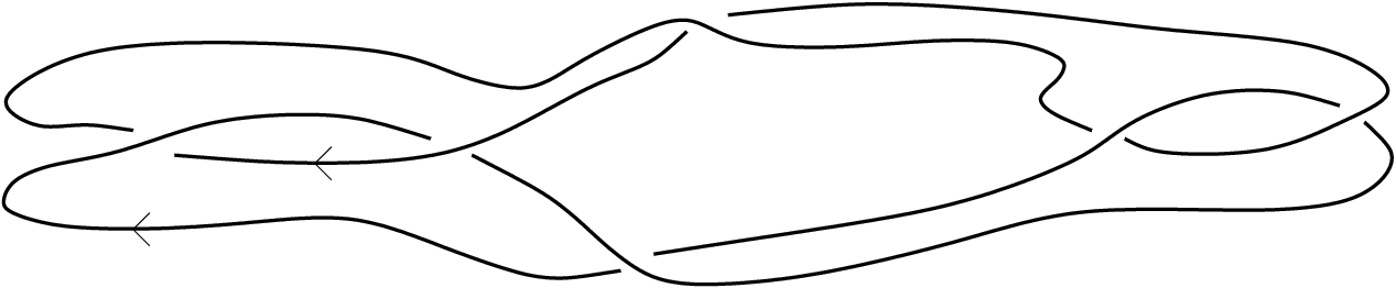



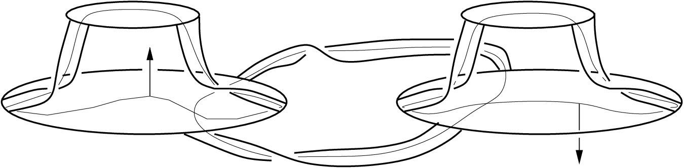
We consider the Seifert graph, with blocks and , from left to right, and the projection surface. We can consider as the block with only one cut vertex. Then, if the positive orientation of is upwards, for the other two blocks the suitable basis is given by the order of blocks , which gives the matrix
Since is a block of type II and the disc that corresponds to the cut vertex is a pan of , according to the proof of Theorem 4 we must add the basis for at the end, obtaining the order and the matrix
3 The box matrix associated to a block
Recall from the introduction that the coefficient of the highest degree term in is equal to and the degree of is , whenever does not vanish. By Theorem 4 where is the Seifert matrix that corresponds to the surface associated to the block of . Then, in order to prove the theorem stated in the introduction, it is enough to show that, if is a block with rank and all its edges have sign , then the determinant of its Seifert matrix does not vanish and has sign . Indeed, since is the sum of the ranks of its blocks, we would have
Now, the part of the diagram that corresponds to a homogeneous block is alternating (in fact, it is a special alternating diagram), and the result for these links follows from the work by Murasugi [15] and Crowell [5] fifty years ago. Murasugi’s proof was accomplished by working on the Alexander matrix of the Dehn presentation, while Crowell worked with the Wirtinger presentation of the fundamental group of the link. In fact, Crowell’s paper rests on a striking application of a graph theoretical result, the Bott-Mayberry matrix tree theorem, an approach which is also explained in Proposition 13.24 of [2]. In this section we will prove it (Theorems 5 and 6) by looking at an explicit matrix of degrees defined using the planar structure of the Seifert graph.
Let be an oriented diagram, its projection surface and the corresponding Seifert graph. Let be a block of . A basis of (hence of ) can be obtained collecting the counterclockwise oriented cycles defined by the boundaries of the bounded regions defined by . Let be the unbounded region defined by this planar graph (see Figure 8).
at 30 150 \pinlabel at 105 105 \pinlabel at 200 105 \pinlabel at 105 40 \pinlabel at -50 150 \endlabellist
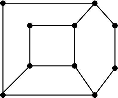
The Seifert graph is a bipartite graph because the projection surface is orientable, hence every circuit in the graph must have an even length. In particular, we can choose a sign for an arbitrary vertex, and extend this labelling to the other vertices in an alternating fashion, when moving along the edges. We also have, for each edge in , its corresponding sign (if the original diagram is homogeneous, this sign is constant in the block). We define as the set of edges in with the sign arrangement shown in Figure 9.
at 195 0 \pinlabel at 118 38 \pinlabel at 65 56 \pinlabel at 195 71 \pinlabel at 333 56 \pinlabel at 195 125 \endlabellist

It turns out that
and
In particular, if the block is homogeneous, let say with sign , then
where is the number of edges in , and
In other words, is the number (with sign ) of the edges in the frontier of the regions and , such that one leaves the signed vertex on the left when going from to through the edge (see Figure 9).
As an example, we display the Seifert matrix associated to the above graph, assuming that the top left vertex is labelled with sign (see Figure 10):
at 30 140 \pinlabel at 108 108 \pinlabel at 200 105 \pinlabel at 105 35 \pinlabel at -50 150 \pinlabel at 4 211 \pinlabel at 188 211 \pinlabel at 58 162 \pinlabel at 149 162 \pinlabel at 250 148 \pinlabel at 45 78 \pinlabel at 180 65 \pinlabel at 255 60 \pinlabel at 0 -10 \pinlabel at 190 -10 \endlabellist
The sets ’s satisfy two properties, which will play later a central role, specially in Theorem 5:
- 1.
If , then , and in particular is the cardinal of the edges in .
- 2.
Consider two consecutive edges and in the boundary of a certain region , that separate from and respectively, with possibly . Suppose that both edges have the same sign, which is the case if we have a homogeneous graph. Then .
\labellist\pinlabelat 112 75 \pinlabel at 259 75 \pinlabel at 112 22 \pinlabel at 259 22 \pinlabel at 184 -10 \endlabellist

Figure 11: Consecutive edges in the boundary of a region
Remark 3.
Note that, for a homogeneous block with sign , the sum of two transposed elements in the corresponding Seifert matrix gives
3.1 The directed dual graph
A description of the Seifert matrix corresponding to a homogeneous block can be better understood as a certain matrix of degrees for the oriented dual graph. To construct the directed dual graph we draw a vertex in the region , including a vertex for the unbounded region , and for each edge in we draw an edge joining and , the edge intersecting the original graph only in . Moreover, the edge is oriented from to if (and only if) . An example is exhibited in Figure 12, assuming the sign for all the edges and for the top left vertex.
at 63 217 \pinlabel at 164 289 \endlabellist

Note that the edges incident at any vertex have alternative orientations, which is equivalent to the second property of the sets ’s. In particular the degrees of the vertices are even numbers.
We now define and where is the number of edges leaving (or going to) and is the number of edges from to . It turns out that the matrix has determinant zero, and we obtain the Seifert matrix of the block by just deleting its last row and column. In the above example, for , we would have
One should note that this is essentially what Proposition 13.21 in [2] states, where the adjective special is applied to a diagram if the union of the black regions (assumed a chessboard colouring in which the unbounded region is white) is the image of a Seifert surface under the projection that defines the diagram.
3.2 Properties of the matrix for a homogeneous block
Let be a sign, or . A square matrix is said to be -signed if its diagonal elements have sign (in particular they do not vanish) and the elements out of the diagonal are zero or have sign . The matrix is said to be row-dominant if for any row we have . The matrix is said to be strictly ascending row-dominant (abbreviated, sard) if is row-dominant and, in addition, there is an order of its rows such that and for any we have that .
The following matrix can be seen to be -signed and sard choosing the order for its rows (note that the condition is for sure if is -signed):
Theorem 5.
Let be a homogeneous block with sign . Then there exists a basis of such that the associated Seifert matrix is -signed and sard.
Proof. Consider the basis of given by the counterclockwise oriented cycles , boundaries of the bounded regions of . Then the Seifert matrix is obviously -signed since where is half the number of edges in the boundary of , and if . To see that is row-dominant note that , and on the other hand , the inequality by the second property of the sets ’s.
We finally check that the matrix is sard, by finding an order for its rows such that for any . By the second property of the sets ’s there is always a bounded region such that . The corresponding row is chosen to be the first one in this order, that is, . Note that, since and , it follows that . Now, when we delete the -th row and column, the remaining matrix corresponds to the graph that remains after deleting the region (precisely, deleting the intersection between and ). The region can be also taken in such a way that the remaining graph is still a homogeneous block, hence the repetition of this process provides the wanted order for the rows of .
3.3 The determinant for a homogeneous block
In this section we will prove that, given a block with sign and rank , the determinant of the corresponding submatrix is non-zero, and its sign is equal to . To see this we just need a final result, purely algebraic, due to Murasugi (see [15], section 2). For the convenience of the reader, we reproduce here its proof in a slightly different way:
Theorem 6.
(Murasugi) Let be a square matrix of order , -signed and sard. Then if and is odd, and otherwise. In other words, does not vanish and has sign .
Proof. By induction on . The case (odd) is trivial; for we have , and the result follows from the fact that is -signed.
Assume now the statement for cases to , and consider the case . Since is sard, there is an order of the rows such that for any we have . In particular, we have that
with and sign . We now develop the determinant by the -row, obtaining
where
and is the determinant of the square matrix of order , obtained by deleting the -th row and column. Since this matrix is also -signed and sard, by induction . Moreover, if each for then obviously; otherwise it is a square matrix of order , -signed and row-dominant, and by Lemma 7 we have that or has sign . Then
and the result follows since and .
Lemma 7.
Let be a square matrix of order , -signed and row-dominant. Then if and is odd, and otherwise.
Proof. For technical reasons in the induction argument, we will prove this result for a slightly wider category of matrices, the weak -signed and row-dominant matrices. For this matrices the condition of being -signed is relaxed for allowing zeros in the diagonal.
We proceed by induction on . The case is trivial. Assume now the statement for cases to , and consider the case . Since is weak -signed and row-dominant, each diagonal element of can be written as with or with sign .
Let be the same matrix as except for possibly the first elements of its diagonal, where we consider instead of just . Let . It turns out that
where the notation is used to denote the matrix obtained from by deleting its -th row and -th column. This follows from the equalities , .
Note that the determinant of is equal to zero, since the sum of all the elements of each row is zero. Moreover, each matrix is also weak -signed and row-dominant, and has order . By induction, its determinant is zero or has sign . Since each is zero or has sign , the result follows.
As an application of the argument developed in this section, we prove the following result:
Claim. Let be an oriented link which has a special alternating diagram. Then the leading coefficient of is if and only if is the connected sum of -torus links.
Proof. Assume that is the connected sum of -torus links. Since , it is enough to show that the leading coefficient of is if is a -torus link. The diagram shown in Figure 13 (left), or its mirror image, is then a diagram of . It has crossings, all with the same sign . The corresponding Seifert graph, shown on the right in Figure 13, is a homogeneous block with two vertices and edges, all of them with sign .

Following the process explained at the beginning of this section, we obtain the Seifert matrix where for , for , and otherwise. Then the leading coefficient of is since .
Suppose now that the leading coefficient of is , and has a special alternating diagram . Then is the connected sum of diagrams where each is a diagram (of a link ) such that its Seifert graph has only one (homogeneous) block (see Figure 14).

Clearly, . Since and , the leading coefficient of each is . Hence it is enough to prove that is a -torus link assuming that the leading coefficient of is , and has a diagram whose associated Seifert graph is a homogeneous block , let say with sign .
We will prove that has the form of the graph shown on the right in Figure 13, by induction on the number of edges of . With this aim, we order the bounded regions of as in the proof of Theorem 5. The corresponding Seifert matrix is then -signed and sard, and by the proof of Theorem 6, we have
where . Since the leading coefficient of is , we have ; since and are nonzero integers, we have .
Now, according to the proof of Theorem 5, is the Seifert matrix associated to the diagram whose Seifert graph is , where is the unbounded region of . Since is still a homogeneous block, by induction we have that has the form of the graph shown on the right in Figure 14, and adds a path connecting the two vertices of in the unbounded region of , as shown in Figure 15.
at 260 115 \pinlabel at 560 115 \endlabellist

Let be the number of edges bounding in . Then the original Seifert matrix is
or its transpose, in any case with determinant . Hence and the result follows.
Corollary 8.
Let be an oriented homogeneous link. Then the leading coefficient of is if and only if is the Murasugi sum of connected sums of -torus links.
4 Homogeneous knots of genus one
We finish the paper with a complete classification of the family of homogeneous knots of genus one. Let be a homogeneous diagram of a homogeneous knot of genus one. Let and be respectively the projection surface and the Seifert graph associated to the diagram . We already know that the genus of is exactly the genus of the knot. Since and is a link with one component, we deduce that has rank two. Figure 16 exhibits the two types of such graphs; they can be denoted by and respectively, where the absolute values of the integers are the numbers of corresponding edges, and their signs are the signs of these edges.
at 25 115 \pinlabel at 115 115 \pinlabel at 205 115 \pinlabel at 330 115 \pinlabel at 510 115 \endlabellist
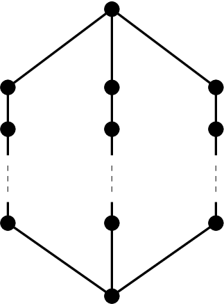
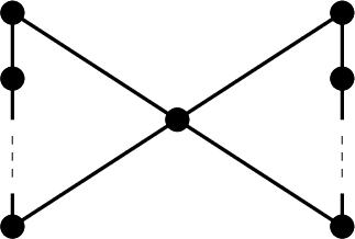
Note that these graphs could have some tails, but this would not affect to the knot type. Since is homogeneous and has only one block, must have all the same sign; since is orientable, they have also the same parity. On the contrary, has two blocks, hence and can have different signs, but both must be even because of the orientability. Note also that the second graph can be considered a degenerated form of the first one, with .
In general, the Seifert graph does not determine the link where it comes from, although in the first case it does. In there are exactly two trivalent vertices; the corresponding Seifert circles can be one inside the other, or separated. When viewed this in the sphere there is no difference, and the corresponding knot is the pretzel knot with diagram . Moreover, since must be a knot, the numbers should be all odd, or exactly one of them should be even. It follows that all of them are odd.
Consider now the graph with two blocks . There is only one vertex with valence four, given the two possible configurations for the Seifert circles shown in Figure 17.
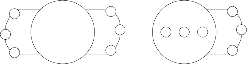
The first configuration corresponds to a link with three components, and the second one corresponds to a knot (Figure 18). Moreover, the obtained knot is also a pretzel knot, given by the pretzel diagram , where and are even integers and is the sign of . For example, is the example in Figure 18, right.


What we have done is to prove the following result:
Theorem 9.
A genus one knot is homogeneous if and only if it belongs to one of the two following classes of knots:
- 1.
Pretzel knots with diagram , where are odd integers with the same sign.
- 2.
Pretzel knots with diagram , where and are non-zero even integers and is the sign of .
The given classification and some partial information of the Jones polynomial allow us to give another proof of the following result, due to Cromwell [4]:
Corollary 10.
Pretzel knots with , all of them odd, are not homogeneous.
In the original proof, Cromwell calculated the Homfly polynomial and checked that contains terms of both signs ([4], Theorem 10). But, for homogeneous links, these coefficients are all non-negative or all non-positive, according to a result by Traczyk ([4], Corollary 4.3).
Proof. We want to prove that the knot defined by a pretzel diagram is not homogeneous. First note that has genus one, since the projection surface defined by the diagram has Euler characteristic , hence genus one, and is not the trivial knot; for example, according to Theorem 2, case (iv) (a) in [11], the span of its Jones polynomial (with normalization ) is , which is different from one since .
Now, the lowest degree and the coefficient of the highest degree term of the Jones polynomial tell us that does not belong to any of the two classes of homogeneous knots of genus one given by Theorem 9, as the following table shows:
Note that the Conway polynomial together with the span of the Jones polynomial are not enough in order to prove Corollary 10. According to the values displayed in the following table, we have for example that the knots defined by the diagrams and share Conway polynomial and the span of their Jones polynomials, and the same happens to the pair of knots defined by the diagrams and .
We also have the following result (as above, the Jones polynomial of the pretzel links and their spans have been calculated following [11]):
Corollary 11.
At least one of the extreme coefficients of the Jones polynomial of a homogeneous knot of genus one is .
Acknowledgments
I am grateful to Prof. Hugh R. Morton for several helpful comments on a previous version of this paper. I am also grateful to the referee for a number of helpful suggestions for the article’s improvement. An overview of this work was presented at Knots in Poland III Conference; I am grateful to its organizers for their hospitality.
The author is partially supported by Spanish Project MTM2010-19355 and FEDER.
References
- [1] Abe, T.: The Rasmussen invariant of a homogeneous knot. Proc. Amer. Math. Soc. 139 (2011), 2647–2656.
- [2] Burde, G. and Zieschang, H.: Knots. De Gruyter Studies in Mathematics, 5. Walter de Gruyter, Berlin-New York, 2003.
- [3] Cromwell, P. R.: Knots and Links. Cambridge University Press., 2004.
- [4] Cromwell, P. R.: Homogeneous links, J. London Math. Soc. 39, 535–552 (1989).
- [5] Crowell, R. H.: Genus of alternating link types, Ann. of Math. 69, No. 2, 258–275 (1959).
- [6] Diestel, R.: Graph theory, Springer-Verlag, Graduate Texts in Mathematics, Vol. 173, 3rd ed., (2006).
- [7] Gabai, D.: Genera of the alternating links, Duke Math. J. 53, 677–681 (1986).
- [8] Gabai, D.: The Murasugi sum is a natural geometric operation, Low-dimensional topology (San Francisco, Calif., 1981), 131–143, Contemp. Math., 20, Amer. Math. Soc., Providence, RI, 1983.
- [9] Jong, I. D. and Kishimoto, K.: On positive knots of genus two. Preprint, 2009.
- [10] Kobayashi, K. and Kodama, K.: On the for plumbing diagrams and oriented arborescent links. Kobe J. Math. 5, no. 2, 221–231 (1988).
- [11]
Manchón, P. M. G.: Kauffman bracket of pretzel links.
Marie Curie Fellowships Annals, Second Volume, 118-122 (2003).
http://www.mariecurie.org/annals/index.html?frame3=/annals/volume2/contents.htm - [12] Mayland, E. J., Jr. and Murasugi, K.: On a structural property of the groups of alternating links. Canad. J. Math. 28, no. 3, 568–588 (1976).
- [13] Melvin, P. M. and Morton, H. R.: Fibred knots of genus two formed by plumbing Hopf bands, J. London Math. Soc. (2) 34, 159–168 (1986).
- [14] Murasugi, K.: On the genus of the alternating knot. I, II. J. Math. Soc. Japan 10, 94–105, 235–248 (1958).
- [15] Murasugi, K.: On alternating knots, Osaka Math. J. 12, 277–303 (1960).
- [16] Murasugi, K. and Przytycki, J. H.: The skein polynomial of a planar star product of two links. Math. Proc. Cambridge Philos. Soc. 106, no. 2, 273–276 (1989).
- [17] Ozawa, M.: Essential state surfaces for knots and links. To appear in J. Austral. Math. Soc.
- [18] Stallings, J. R.: Constructions of fibred knots and links. Proc. Sympos. Pure Math. Stanford Univ. 1976, Part 2, 55–60, (1978).
- [19] Stoimenow, A.: Knots of (canonical) genus two. Fund. Math. 200 (1), 1–67 (2008).
Pedro M. González Manchón
Department of Applied Mathematics
Ronda de Valencia 3
EUITI-UPM
28012 Madrid (Spain)
pedro.gmanchon@upm.es
http://gestion.euiti.upm.es/index/departamentos/matematicas/manchon/index.htm