Constraining the dark energy equation of state using LISA observations of spinning Massive Black Hole binaries.
Abstract
Gravitational wave signals from coalescing Massive Black Hole (MBH) binaries could be used as standard sirens to measure cosmological parameters. The future space based gravitational wave observatory Laser Interferometer Space Antenna (LISA) will detect up to a hundred of those events, providing very accurate measurements of their luminosity distances. To constrain the cosmological parameters we also need to measure the redshift of the galaxy (or cluster of galaxies) hosting the merger. This requires the identification of a distinctive electromagnetic event associated to the binary coalescence. However, putative electromagnetic signatures may be too weak to be observed. Instead, we study here the possibility of constraining the cosmological parameters by enforcing statistical consistency between all the possible hosts detected within the measurement error box of a few dozen of low redshift () events. We construct MBH populations using merger tree realizations of the dark matter hierarchy in a CDM Universe, and we use data from the Millennium simulation to model the galaxy distribution in the LISA error box. We show that, assuming that all the other cosmological parameters are known, the parameter describing the dark energy equation of state can be constrained to a 4-8% level (2 error), competitive with current uncertainties obtained by type Ia supernovae measurements, providing an independent test of our cosmological model.
Subject headings
black hole physics – gravitational waves – cosmology: cosmological parameters – galaxies: distances and redshifts – methods: statisticalI. Introduction
The Laser Interferometer Space Antenna [10, LISA,] is a space based gravitational wave (GW) observatory which is expected to be launched in 2022+. One of its central scientific goals is to provide information about the cosmic evolution of massive black holes (MBHs). It is, infact, now widely recognized that MBHs are fundamental building blocks in the process of galaxy formation and evolution; they are ubiquitous in nearby galaxy nuclei [28, see, e.g., ], and their masses tightly correlate with the properties of their host [15, and references therein]. In popular CDM cosmologies, structure formation proceeds in a hierarchical fashion [48], through a sequence of merging events. If MBHs are common in galaxy centers at all epochs, as implied by the notion that galaxies harbor active nuclei for a short period of their lifetime [16], then a large number of MBH binaries are expected to form during cosmic history. LISA is expected to observe the GW driven inspiral and final coalescence of such MBH binaries out to very high redshift with high signal-to-noise ratio (SNR), allowing very accurate measurements of the binary parameters. The collective properties of the set of the observed coalescing binaries will carry invaluable information for astrophysics, making possible to constrain models of MBH formation and growth [33, 14, 39].
Besides astrophysical applications, coalescing MBHs could be used as standard sirens [38, 18, 20, 2, 3, 21, 44]. The high strength of the GW signals allows us to measure the luminosity distance with a precision of less than a percent at redshift (neglecting weak lensing). However, we need an electromagnetic identification of the host in order to measure the source redshift and be able to do cosmography. If the event is nearby (), then we have a very good localization of the source on the sky and we can identify a single cluster of galaxies hosting the merger. As we go to higher redshifts, LISA sky localization abilities become quite poor: a typical sky resolution for an equal mass inspiralling MBH binary at is 20-30 arcminutes a side at [42, 21, 1], which is in general not sufficient to uniquely identify the host of the GW event. There is, therefore, a growing interest in identifying putative electromagnetic signatures associated to the MBH binary before and/or after the final GW driven coalescence [for a review, see 37, and references therein]. Electromagnetic anomalies observed before or after the coalescence within the LISA measurements error box may allow us to identify the host and to make a redshift measurement. However, most of the proposed electromagnetic counterparts are rather weak (below the Eddington limit), and in case of dry mergers (no cold gas efficiently funneled into the remnant nucleus) we do not expect any distinctive electromagnetic transient. This brings us back to the original idea by [38] to consider each galaxy within the LISA measurement error box as a potential host candidate. The idea is that, by cross-correlating several GW events, only one galaxy (cluster of galaxies) in each error box will give us a consistent set of parameters describing the Universe. The effectiveness of this method has been demonstrated by [26] in the context of the Hubble constant determination by means of low redshift () extreme mass ratio inspirals.
We use the hierarchical MBH formation model suggested by [45] to generate catalogs of coalescing MBH binaries along the cosmic history. This model predicts MBHs mergers observable by LISA in three years, in the redshift range . We do not use sources beyond redshift due to difficulties of measuring galaxy redshifts beyond that threshold11 1 There are other reasons for not going beyond which we will discuss later.. We model the galaxy distribution in the Universe using the Millennium simulation [41]. For each coalescing MBH in our catalog, we select a host galaxy in the Millennium run snapshot closest in redshift to the actual redshift of the event. For each galaxy in the snapshot, we compute the apparent magnitude in some observable band, and we create a catalog of redshift measurements of all the observable potential host candidates. Note that typical observed mergers involve MBHs, which implies [15, using the black hole mass–bulge relations, see, e.g., ] relatively light galaxies. However, observed galaxies are heavy due to selection effects: roughly speaking, mass reflects luminosity, so that at high redshifts we can observe only very massive (luminous) galaxies. Therefore, the actual host might not be (and often is not) among the observed galaxies. The important fact is the self-similarity of the density distribution: the local density distribution for all galaxies and the density distribution for heavy galaxies are quite similar, which allow us to infer the likelihood of the host redshift on the basis of redshift measurements of the luminous galaxies only.
We assume that the GW source parameter measurements (GW likelihoods) are represented by multivariate Gaussian distributions around the true values, with the variance-covariance matrix defined by the inverse of the Fisher matrix. This is a good approximation in the case of Gaussian instrumental noise and large SNR. At the uncertainty in the luminosity distance () is dominated by weak lensing due to the extended distribution of dark matter halos between us and the GW source. In this paper we combine the luminosity distance errors given by GW measurements and weak lensing, referring to them as GW+WL errors. We use two estimations of the weak lensing error (i) from [40] and (ii) from [47].
In order to evaluate the error box we need to assume some prior on the cosmological parameters. In this exploratory study, we assume that we know all the cosmological parameters but the effective equation of state for the dark energy, described by the parameter (which could be the case by the time LISA will fly). In a follow up paper we will relax this assumption by including also the Hubble constant and the matter and dark energy content of the Universe as free parameters. We take the prior range for from the seven-year WMAP analysis [19]. We show that using statistical methods can be constrained to a 4-8% level (2 error ), providing an effective method for estimating the dark energy equation of state. We also show that this result depends weakly on the prior range and could serve as an independent way of measuring the dark energy equation of state, with respect to canonical methods employing observations of type Ia supernovae [34].
The paper is structured as follows. In Section II we spell out explicitly all the details of the adopted cosmological model and of the Bayesian analytical framework. In Section III we give more insights on the MBH population model and on the galaxy distributions extracted from the Millennium database. In Section IV we describe our simulated GW and electromagnetic observations. We give results of our simulations under different assumptions about weak lensing, depth of the follow up electromagnetic surveys, etc. in Section V. We summarize our findings in Section VI.
II. Analytical framework
II.1. Cosmological description of the Universe
We assume the standard model, which describes our Universe as the sum of two non-interacting components: (i) a pressureless component corresponding to all visible and dark matter, (ii) a dark energy component with current effective equation of state corresponding to the term . Current estimates based on SN1a observations and anisotropy measurements in the cosmic microwave background [34, 19] tell us that about 70% of the Universe energy content is in the form of the dark energy. The evolution of the Universe is therefore described by the expansion equation
| (1) |
where ( being the lengthscale of the Universe) is the Hubble expansion parameter and is its current value (), and are the ratios of the matter density and the dark energy density to the critical density, and describes the effective dark energy equation of state as a function of . We assume that the Universe is spatially flat, the luminosity distance is therefore computed as
| (2) |
In our simulations we fix all parameters (assuming that they are known exactly) to the currently estimated mean values: , . We also simplify the form of for which we will assume , where is a constant 22 2 Here we use notations for the dark energy equation of state adopted in the WMAP data analysis [19].. We choose the value to simulate our Universe which is what has been used in the Millennium simulation (see below).
II.2. Methodology and working plan
Our aim is to show that we can constrain via GW observations of spinning MBH binaries, using a Bayesian framework. Let us consider GW observations. For each event we can infer the probability of a parameter , given the collected data , using Bayes theorem:
| (3) |
Here is the posterior probability of the parameter , is the likelihood of the observation given the parameter , in the prior knowledge of and is defined as
| (4) |
The likelihood must be appropriately specialized to our problem. We want to exploit GW observations to constrain through the distance - redshift () relation as given by (2).
- •
The distance is provided by the GW observations: the GW signal carries information about the parameters of the binary, including its location on the sky and its luminosity distance. All those parameters can be extracted using latest data analysis methods [32, 9]. The measurements errors are encoded in the GW likelihood 33 3 Through the paper, with GW likelihood we mean the likelihood of the LISA data to contain the GW signal with a given parameters, not to be confused with the likelihood defined in the Bayes theorem. function , where are the ecliptic coordinates of the source and represents all the other parameters characterizing MBH binary (spins and their orientation, masses, orientation of the orbit and MBHs position at the beginning of observations). When estimating weak lensing can not be neglected. In fact the error coming from the weak lensing (causing fluctuations in the brightness of the GW source which gives an uncertainty in the luminosity distance) dominates over the GW error starting from redshift (see figure 2).
- •
The redshift measurement does not rely on any distinctive electromagnetic signature related to the GW event. We extract a redshift probability distribution of the host from the clustering properties of the galaxies falling withing the GW+WL error box. This defines an astrophysical prior for a given galaxy in the measurement error box to be the host of coalescing binary. To translate the measured and uncertainty of the GW event into a corresponding and for the candidate host galaxies in the sky we use the prior knowledge of obtained from WMAP.
The likelihood in equation (3) can therefore be written as
| (5) |
where we have introduced the priors on the parameters (which we assume in this paper to be uniform). It is convenient to change the variable of integration from to . Since we have assumed uniform priors on , we can marginalize the likelihood over those parameters 44 4 Here this corresponds to the projection of the Fisher matrix to three dimensional parameter space of sky location and luminosity distance . to obtain:
| (6) |
where we denoted the marginalized GW likelihood as . Practically, we limit the integration to the size of the error box (in principle the integration should be taken over the whole range of parameters but we found that considering the error box is sufficient).
We assume that the error in luminosity distance from the weak lensing is not correlated with the GW measurements, hence the integral in equation (6) can be performed over the sky () first, and then over the redshift. We also found that the correlation between and the sky position coming from the GW observations is not important for events at . Plugging equation (6) into equation (3) defines the posterior distribution of for a single GW event (as indicated by the index ). Assuming that all GW events are independent, the combined posterior probability is
| (7) |
To evaluate through equation (7) we therefore need:
- •
a MBH binary population model defining the properties of the coalescing systems;
- •
the spatial distribution of galaxies within a volume comparable with the combined GW+WL measurement error box;
- •
the measurement errors associated to GW observations of coalescing MBH binaries (defining );
- •
an estimation of spectroscopic survey capabilities to construct the galaxy redshift distribution within the GW+WL measurement error box (defining ).
We will consider these points individually in the next two sections.
III. Astrophysical background
III.1. Massive black hole binary population
To generate populations of MBH binaries in the Universe, we use the results of merger tree simulations described in details in [46]. MBHs grow hierarchically, starting from a distribution of seed black holes at high redshift, through a sequence of merger and accretion episodes. Two distinctive type of seeds have been proposed in the literature. Light () seed are thought to be the remnant of Population III (POPIII) stars [27], whereas heavy seeds form following instabilities occurring in massive protogalactic disks. In the model proposed by Begelman Volonteri & Rees [5, hereafter BVR model], a ‘quasistar’ forms at the center of the protogalaxy, eventually collapsing into a seed BH that efficiently accretes from the quasistar envelope, resulting in a final mass few . Here we use the model recently suggested by Volonteri & Begelman [45, hereafter VB model], which combines the two above prescriptions by mixing light and heavy initial seeds. This model predicts events per year in the redshift range , relevant to this study.

The dashed blue lines in figure 1 show the redshifted total mass (, being the restframe masses of the two MBHs, upper–left panel), mass ratio (, upper–right panel) and redshift (lower panel) distribution of the MBH binaries coalescing in three years, as seen from the Earth. The model predicts coalescences in the redshifted mass range , almost uniformly distributed in the mass ratio range , with a long tail extending to . For comparison we also show the population expected by a model featuring heavy seed only (BVR model, green dotted–dashed lines), and by an alternative VB type model (labeled VB-opt for optimistic, red long–dashed lines) with a boosted efficiency of heavy seed formation [see 45, for details]. It is worth mentioning that these models successfully reproduce several properties of the observed Universe, such as the present day mass density of nuclear MBHs and the optical and X-ray luminosity functions of quasars [29, 35]. The BVR and the VB-opt models predict MBH population observables bracketing the current range of allowed values. The VB-opt model, in particular, is borderline with current observational constraints on the unresolved X-ray background, and it is shown here only for comparison. In the following, we considered the VB model only, which fits all the relevant observables by standing on the conservative side.
We performed 100 Monte Carlo realizations of the population of MBH binaries coalescing in three years. Each realization takes into account the distribution of the number of events and MBH masses with the redshift as predicted by the VB model. Other parameters (like time of coalescence, spins, initial orbital configuration) are chosen randomly using uniform priors over the appropriate allowed ranges.
III.2. Galaxy distribution
To simulate the galaxy distribution in the Universe we use the data produced by the Virgo Consortium publicly available at http://www.g-vo.org/Millennium. These data are the result of the implementation of semi-analytic models for galaxy formation and evolution into the dark matter (DM) halo merger hierarchy generated by the Millennium simulation [41]. The Millennium run is a N-body simulation of the growth of DM structures in the expanding Universe starting from a Gaussian spectrum of initial perturbations in the DM field at high redshift, which successfully reproduced the net-like structure currently observed in the local Universe. The simulation has a side-length of Mpc (co-moving distance), and its outcome is stored in 63 snapshots evenly separated in log(), enclosing all the properties of the DM structure at that particular time. Semi-analytical models for galaxy formation are implemented a posteriori within the DM structures predicted by the simulation. Such models have been successful in reproducing several observed properties of the local and the high redshift Universe [8, 12, see , e.g.,]. Here we use the implementation performed by Bertone and collaborators [6], which is a refinement of the original implementation by [12].
For each coalescing MBH binary, we choose the snapshot closest in redshift. Within the snapshot we choose the host of the GW signal according to a probability proportional to the number density of neighbor galaxies . Such assumption comes from the fact that two galaxies are needed in order to form a MBH binary, and we consider that the probability that a certain galaxy was involved in a galaxy merger is proportional to the number of neighbor galaxies. We consider to be neighbors of a specific galaxy all the galaxies falling within a distance
| (8) |
where km s-1 is the typical velocity dispersion of galaxies with respect to the expanding Hubble flow, and is the Hubble time at the event redshift. The number density of neighbor galaxies is then simply written as . When we choose the merger host, we compute considering all the neighbor galaxies, without imposing any kind of mass or luminosity selection. In this case . However, when we will construct the probability of a given observable galaxy to be the host of the merger (i.e. the astrophysical prior ), we will have to compute according to the number of observed neighbors, because this is the only thing we can do in practice when we deal with an observed sample of galaxies (see Section IV.2).
IV. Simulating the observations
IV.1. Gravitational wave observations: shaping the error box
As we mentioned in Section III.1, we drawn hundred realizations of the MBH binary population from the VB model. Each realization contains 30 to 50 events in the redshift range . The total mass, mass ratio and redshift distributions of the events are shown in the figure 1. In order to simulate GW observations, the binary sky location is randomly chosen according to a uniform distribution on the celestial sphere, the coalescence time is chosen randomly within the three years of LISA operation (we assume 3 years as default mission lifetime). the spin magnitudes are uniformly chosen in the interval in units of mass square, and the initial orientations of the spins and of the orbital angular momentum are chosen to be uniform on the sphere. More detailed description of the model for GW signal used in this paper is given in [32].
The GW likelihood needed in equation (5) is approximated as a multivariate Gaussian distribution with inverse correlation matrix given by the Fisher information matrix (FIM) :
| (9) |
Here is the vector of the parameters characterizing the spinning MBH binary, are the maximum likelihood estimators for those parameters which are assumed to correspond to the true values (no bias), and is the FIM, where the commas correspond to derivatives with respect to the parameters. This is a reasonable approximation due to the large SNR [43, for more details on the FIM and its applicability see]. Our uncertainties on estimated parameters are consistent with [21], [4] and [32]. We did not include higher harmonics (only the dominant, twice the orbital frequency) as they only slightly improve parameter estimation for precessing binaries. However including higher harmonics in the GW signal model is important in case of the small spins and low precession (when spins are almost (anti)aligned with the orbital momentum, [22]). We use truncated waveforms corresponding to the inspiral only. However the addition of merger and ring-down will further reduce the localization error due to the higher SNR [30]. This error is usually an ellipse on the sky but we simplify it by choosing the circle with the same area.
For the luminosity distance measurement we need to take into account the weak lensing. We assume the weak lensing error to be Gaussian with a given by (i) [40]. Such assumption is rather pessimistic; we also tried the prescription given by (ii) [47], which gives smaller errors, but still larger than the level that may be achieved after mitigation through shear and flexion maps [17]. Both of those estimations are represented in figure 2 as (i) dark (red online) circles and (ii) light (orange online) squares correspondingly. The median error in due to GW measurements only is given by the solid black line. The combined error for model (i) is given by the upper (blue) circle-line curve, and for model (ii) by the lower (green) square-line curve.

We consider our setup to be conservative in the estimation of the weak lensing effects. The main aim of this work is to build a reasonable setup for what could be observed by the time LISA will fly, and make a first order estimation of LISA capabilities to constrain the dark energy equation of state. We will address non-Gaussianity of the weak lensing as well as other corrections to the model to make it more realistic in a follow up paper.
We consider an error box size corresponding to of the measurement errors in the sky location () and in the source distance as evaluated by the FIM plus weak lensing uncertainties. For observational purposes, the dimensions of this error box are and . For the latter we also include the uncertainty given in the conversion due to the error (prior) on , .
Let us summarize how we construct an error box in practice, as, for example, the one illustrated in figure 3 :
- •
We select the closest Millennium snapshot to the event in redshift.
- •
We pick a galaxy (red dot) in the snapshot with a probability given by the local galaxy number density .
- •
We construct around the galaxy an error box given by and , and the galaxy can lie anywhere with respect to this error box (blue cylinder).
- •
We expand the error box along the direction of the observer both sides by given by the uncertainty in (green cylinder).
- •
According to some prescription,which we will describe in the next section, we select observable galaxies in the error box (brown dots).

As shown in figure 3, we interpret one of the directions in the Millennium snapshot as distance from the observer, and convert the comoving distance in redshift. We assume a periodic expansion of the Millennium data in order to fit large error boxes. Note that the original Millennium simulation also assumes the same periodicity in the distribution of the matter. The size of the error box at high redshift covers a significant fraction of the simulation box so we do not go beyond the redshift (as we will show later, spectroscopic observations at such high redshifts will be impractical anyway). Together with larger error boxes, we have a nonlinear increase in the number of events at high redshift. To reduce the overlap between error boxes corresponding to different GW events we choose cylinders with random orientations.
Figure 4 shows an example of the resulting weighted distribution of galaxy redshifts (with weight proportional to the local density ). It is a projection of the clumpiness along the line of sight which is also proportional to the probability distribution of for the event. The probability distribution of for the event will be directly related to this result. We noticed that there is a very large number of underdense regions and several very dense superclusters. The probability of a galaxy with a low local density to host a merger is very low but there is a huge number of such galaxies, and we found that the probability of the host to be in (super)clusters is similar to that of being in a low density region. As we will see later in the result section, this may cause a very wrong estimation of for some individual GW event.

IV.2. Redshift measurements through spectroscopic surveys
To get a statistical measurement of we need to exploit the clustering of the galaxies falling within the error box (which defines the astrophysical prior in equation (5)). It is therefore necessary to get efficient redshift measurements of thousands of galaxies within a small field of view (FOV): the information we seek is enclosed in the redshift distribution of such galaxies. We stress here that we are not looking for a distinctive electromagnetic counterpart to the GW event. In fact, the actual host of the coalescing binary may not even be observable. Typical masses of our binaries are . Using MBH-bulge scaling relations [15], such MBHs are expected to be hosted in galaxies with stellar mass , i.e., in dark matter halos with total mass . The Millennium run mass resolution is , meaning that typical host structures are formed by less than 100 particles. Unfortunately, the Millennium run is severely incomplete in the expected mass range of LISA MBH binary hosts. Here we do not attempt to exploit any MBH-host relation to select the host of our GW event; the probability of being a host is only related to the local number density of neighbor galaxies . Such assumption relies on the concept of self-similarity of the galaxy clustering at different mass scales: typical LISA MBH binary hosts cluster in the same way as more massive galaxies. We checked this assumption by comparing the spatial distribution of galaxies in different mass ranges (, , ), within simulation snapshots at different redshift, and we postulate that this self-similarity extends to lower masses, below the Millennium run resolution. This point is crucial for two reasons: (i) especially at , we will be able to get only spectra of luminous (massive) galaxies, and we need to be confident that their spatial distribution mimics that of lighter galaxies that may host the GW event but are observable in the spectroscopic survey; (ii) the number of observable galaxies in the error box may be too large anyway () to efficiently complete a spectroscopic survey on the full sample: self-similarity allows us to get the clustering information we need by getting spectra of the brightest objects only.
At , the typical number of galaxies enclosed in the 2 error box described above is in the range . However, not all of them are bright enough to get useful spectra. The semianalytic galaxy evolution model [6] implemented on top of the Millennium run returns the stellar mass of each galaxy, and the absolute bolometric magnitude . By knowing the redshift, and by using standard galactic templates one can therefore compute the apparent magnitude in a given band, by assuming the appropriate correction [31]. Here we use the band apparent magnitude for illustrative purposes, and we adopt the relation [49]
| (10) |
where 0.6 is the correction. For each galaxy we compute and we simulate spectroscopic surveys at different thresholds . We stress here that the GW host was chosen among all the galaxies falling in the error box, and therefore may not (and usually does not) belong to the observed sample. We then assume that for each galaxy satisfying the survey threshold we get an exact spectroscopic redshift, and we combine the redshift distribution of several error boxes to get a statistical estimation of . In practice, each redshift estimation will come with a measurement error, and an intrinsic error due to the proper motion of the source with respect to the Hubble flow. Both errors are however of the order of , well below the typical redshift scale corresponding to spatial clustering of structures (, see figure 4) we need to resolve.
Our method does not rely on the observation of a prompt transient associated to the MBH binary coalescence to identify the host galaxy. Nevertheless, getting thousands (or tens of thousands) of spectra in a small field of view requires a dedicated observational program. Thanks to multi-slit spectrographs such as VIMOS at VLT [23] and DEIMOS at Keck [13], fast deep spectroscopic surveys of relatively large FOV are now possible. For example, the ongoing VIMOS VLT deep survey [24], took spectra of galaxies, mostly in the redshift range , within a FOV of 0.61deg2 at an apparent magnitude limit . Comparable figures are achieved by other observational campaigns such as zCOSMOS [25] and DEEP2 [11], being able of surveying selected galaxies in various photometric bands () to an apparent magnitude limit of about 24. Going deeper in redshift, Lyman break galaxy redshift surveys are being successful in efficiently getting high quality spectra of hundreds of galaxies in the redshift range within a FOV deg2 [7]. To get an idea, the VIMOS spectrograph can take high quality spectra per pointing with an integration time of about h, within a 78 arcmin2 FOV, which is coincidentally of the same order of the typical error box for a GW event. The typical redshift accuracy of the spectra is ( in the zCOSMOS survey, in the Lyman break galaxy survey), well below the typical redshift scale we are interested in ().
Such figures witness the feasibility of efficient spectroscopic redshift determination of a large sample of galaxies at faint apparent magnitude (), as required by our problem. Future spectroscopic survey as BigBOSS [36] are expected to further improve such figures of merit; a new spectrograph will be able to simultaneously get up to 4000 spectra within a single pointing of a 7deg2 FOV. Getting few thousand spectra of objects falling within the GW error box in the redshift range of interest may be possible in a single observing night. At a cut-off magnitude we generally have few hundred to few thousands galaxies in the GW error box, but we go deeper (i.e., , feasible with future surveys), the number of spectra may increase drastically. For some of the error boxes, we count up to galaxies with . However, the requirement of a factor of ten more spectra, does not correspond to a significant improvement of the results. This is a consequence of the self similarity of the galaxy distribution: as long as there are enough galaxies in the error box to recover the clustering information, the results are basically independent on the assumed cut-off magnitude. A survey with a cut-off magnitude of may indeed be a good compromise between reliability of the results and time optimization in terms of follow-up spectroscopy.
The magnitude cut-off defines the number of neighbor observable galaxies. This is the only practical way to weight each galaxy with a local density, (the subscript refers to the adopted magnitude limit) along the lines discussed in Section . Once we have a spectroscopic galaxy sample, each galaxy in the error box comes with the prior probability to be the host proportional to , so the astrophysical prior in equation (6) could be written as
| (11) |
where the sum is over all observable galaxies in the error box and is the geodesic distance on the celestial sphere from the center of the box. At redshifts the prior probability becomes almost a continuous function (as the example in figure 4).
IV.3. Approximations and caveats
Before jumping to the results, we want to mention some corrections we made to accommodate the limitations of our simulations. Firstly, we interpreted one of the directions in the snapshot (along the side of the cylinder) as distance from the observer. This is a good approximation only if the error box size is small. For large error boxes, a uniform distribution in the comoving distances does not translate into a uniform distribution in redshifts: there is an artificial slope with a bias toward low values of . We have corrected for this slope. Secondly, the clumpiness evolves with redshift, which is not the case if we use a single snapshot and interpret one of the directions as a redshift. To properly account for this, we should glue snapshots together and perform an interpolation between them. However we wanted to simplify the setup for this very first attempt. The main idea was to check whether the density contrast within the error boxes is sufficient to constrain further the error on . If the distribution of density within the error box is uniform then we do not gain any useful information. However there is a natural bias: for a given measurement of , the galaxy further away (larger ) constrains better than galaxy at lower redshift. One can see it from the fact that deviation between the curves in plane corresponding to the small deviation in is bigger for large . This could be counterbalanced by the decreasing density contrast at large redshift. Here, we corrected the slope of the posterior by demanding that a uniform distribution returns a posterior on equal to the prior, i.e., .
V. Constraints on the dark energy equation of state
In this section we present the results of our simulations. We tried several setup of the experiment by using different thresholds on the observable apparent magnitude of galaxies, different prescriptions for the measurement errors, and different cosmological priors. For each setup, we performed either 100 or 20 realizations of the MBH binary population as observed by LISA, together with the follow up spectroscopic survey of the galaxies in all the error boxes.
V.1. Fiducial case
We consider in this subsection 100 realizations which we refer to as our fiducial case. For this setup, we limit spectroscopic identification of galaxies in the error box to an apparent magnitude of , the errors in sky localization and in the luminosity distance are estimated according to the inspiral part of GW signal only, and the weak lensing uncertainty is taken from [40]. The prior was assumed to be uniform with an exponential decay at the boundaries. Such interval is consistent with current (95% confidence level) constraints on [19, ,], obtained by cross correlating seven-year WMAP data with priors coming from independent measurements of and barionic acoustic oscillations [see 19, and references therein for full details], under our same assumption for the dark energy equation of state, , where is a constant. Such range is reduced by a factor of almost three () when type Ia supernovae data [34] are included. Here we show that GW measurements offer a competitive alternative to type Ia supernovae, placing an independent constraint on the dark energy equation of state.
We find that in almost all cases we improve the constraints on , in other words, the posterior distribution is narrower than the prior. Few events at low redshift usually play a major role in the final result. One typical realization is plotted in the top panel figure 5. We split the contribution to the posterior distribution in redshift bands: (second plot from the left), (third plot), (fourth plot). Their relative contribution and the resulting posterior (black) is given in the leftmost plot. In this example the final posterior probability is almost completely determined by few events at low redshift. The second realization, shown in the lower panels of figure 5, demonstrates how low redshift contributions could give inconclusive results. In this particular case, there are two maxima with preference given to the wrong one. The contribution from high redshift events could change this ratio as it is shown in this example. In many cases the mergers above redshift can constrain only to a 0.1-0.15 accuracy, but they almost always add up coherently giving a maximum at the right value (). This usually helps in case the low redshift events return a multimodal , and is, in turn, the power of our statistical method.
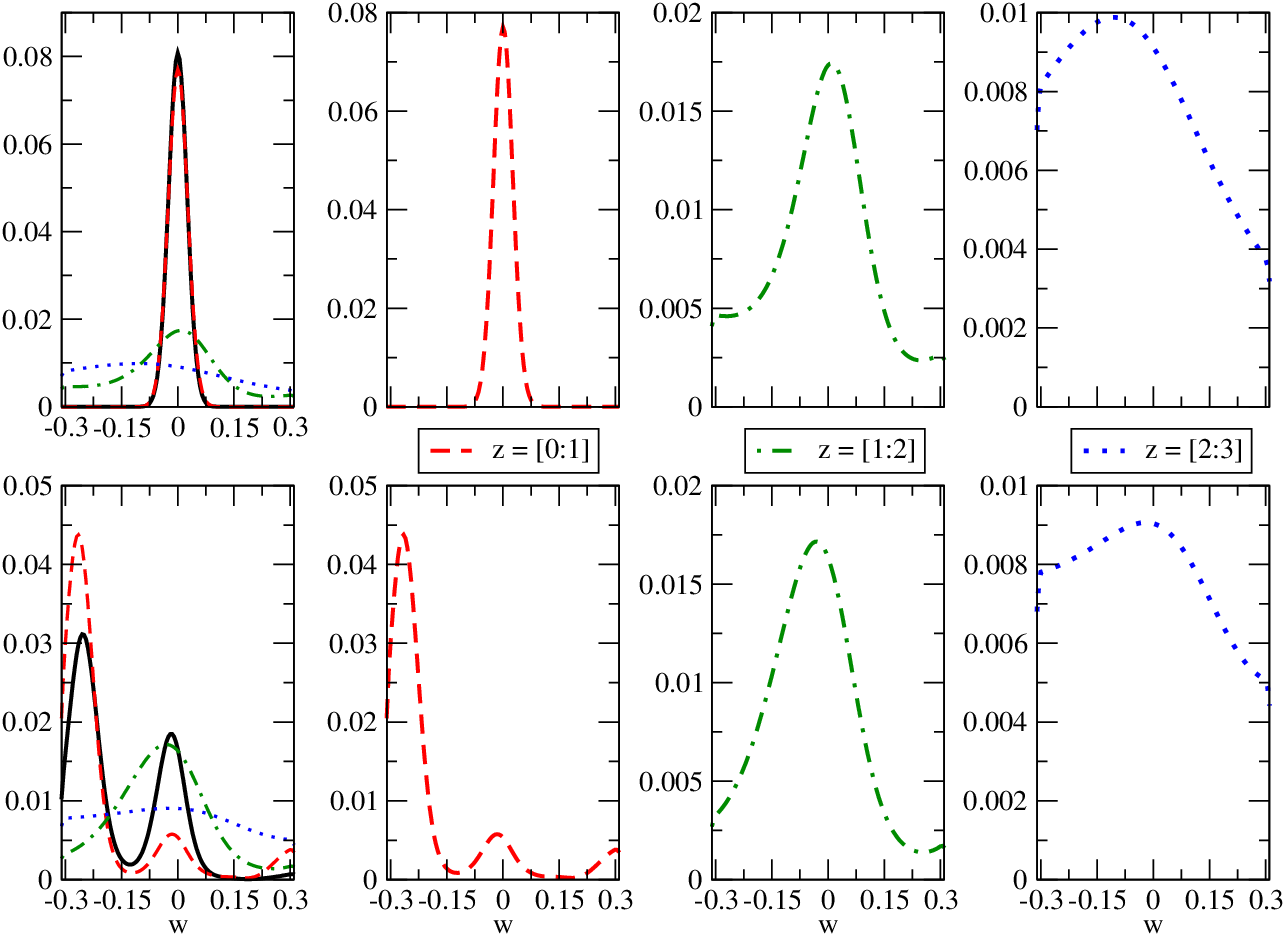
We characterize the results of each setup (100 or 20 realizations) using the figures of merit shown in figures 6 and 7. The first one (figure 6) is obtained by adding the posterior distributions of all the realizations. We fit the resulting curve with a Gaussian, characterizing the result using its mean and standard deviation . The second figure of merit (figure 7) shows the result of Gaussian fits performed on each individual realization (vertical index ): the mean is shown as a circle and the standard deviation is the error bar. The first figure of merit gives collective information, showing how well, on average, an individual realization can be approximated by a Gaussian fit, while the second figure of merit shows the dispersion of the posterior distribution across the individual realizations.
The fiducial case, featuring 100 realizations, is shown in panel (a) of both figures 6 and 7. The parameters of the global fitting Gaussian mean are and , corresponding to a factor of four improvement in the estimation of with respect to our standard prior. However the distribution has clearly some outliers, recognizable as non-Gaussian tails in figure 6 and pinned down in figure 7.
 |
 |
 |
 |
 |
 |
For the fiducial case, 84% of the realizations have a mean value close to the true one, i.e. with an appreciable reduction of the prior range, i.e. ( is the realization index). Moreover, most of the outliers can be corrected as we will explain in Section V.6.

V.2. Removing “electromagnetic counterparts”
Our goal is to demonstrate that we are able to constrain the dark energy equation of state without directly observing electromagnetic counterparts. However, for some of the low redshift events, the error box is so small that only one or two galaxies fall within it. Having one or two galaxies in the error box essentially implies an electromagnetic identification of the host, so we decided to re-analyze the fiducial case removing all such fortunate events (usually 0-2 in each realization). The fiducial case without clearly identifiable hosts is presented in the panel (b) of figure 6. Clearly, our results remain almost unchanged, the posterior distribution is slightly wider (larger sigma) and non-Gaussianity is more pronounced.
V.3. Choice of the prior for
Here and in the next subsections we make use of 20 selected realizations, which we found to be sufficient to depict the relevant trends of the analysis. We took 15 “good” (mean values close to the true and small rms errors) and 5 “bad” cases from the fiducial setup.
In this subsection we study the effect of the prior on the posterior distribution. We considered an extreme case: a Gaussian . As shown in panel (c) of figure 6, the global posterior distribution is still centered at the true value . This demonstrates that the final conclusion is basically unaffected by the choice of the prior (as long as the prior covers the true value) and GW observations, in principle, could be used as an independent mean of estimating .
V.4. Using deeper surveys
Here we study the dependence of our results on the depth of the follow up spectroscopic survey: i.e. on the observability threshold. We considered the same 20 realizations as in the previous section, but now with different limits on the apparent magnitude of observable galaxies: . The case is given in panel (d) of figures 6 and 7. The results are comparable to the fiducial case. They show a small improvement in sigma and slightly larger bias for the combined distribution. We also notice that 4 out of 5 “bad” cases remain bad.
We should say few words about the number of galaxies used here. As mentioned above, the typical number of galaxies for the fiducial case () is less than few thousand for events at and less than few tens of thousands for the high redshift event. For the improved observational limit (), these numbers are 2 to 10 times larger. The fact that our results are not sensitive to the depth of the survey reflects the self-similarity of the spatial distribution of galaxies in different mass ranges.
V.5. Improving the sky localization and the luminosity distance estimation
In our fiducial setup, the assumed source sky localization and luminosity distance error are rather conservative. In this subsection we consider the effect of improving such measurements. So far, we considered only the inspiral part of the GW signal; the inclusion of merger and ringdown will improve the localization of the source by at least a factor of two [30], due to the large gain in SNR. We artificially reduced the sky localization error coming from the inspiral by a factor of two (factor of four in the area), assuming that this will be the case if we take the full GW signal. We reanalyzed the same 20 realizations with this new error on the sky. Because the size of the error box is smaller, the number of potential counterparts is reduced by a factor of compared to the fiducial case. The results are presented in panel (e) of figure 6. We see that the main effect of a better GW source localization is to reduce the number of outliers and to remove the non-Gaussian tails in the combined probability. As it is clear form panel (e) of figure 7, the main gain comes from improvement of the “bad” cases.
We now consider another estimation of the mean weak lensing contribution to the luminosity distance error, given in [47] (green square-line curve on figure 2). We take this in combination with improved source localization on the sky coming from taking into account the merger (as discussed above). We consider the same 20 realizations. Results are shown in panel (f) of both figures 6 and 7. The improvement with respect to all the other cases is obvious. Because the marginalized likelihood coming with each galaxy is narrower due to the smaller error in the luminosity distance, the final posterior on is also narrower. The standard deviation is improved by more than 40% as compared to the fiducial case. The non-Gaussian tails have almost completely disappeared, due to the removal of the outliers (further improvement of the “bad” cases, the remaining bad case will be treated in the subsection V.6, see also the top panel of figure 8). With this model of the mean weak lensing contribution and assuming the full GW signal, the estimation of is improved by a factor of as compared to the initial uniform prior.
V.6. Consistency check.
As we mentioned above, some nearby GW event could seriously bias the final posterior. We also mentioned that the odds for the host to be in a low density region of the Universe are not small. The posterior probability reflects the distribution of the mass defined by the astrophysical prior . A nearby GW event hosted in the low density environment could seriously damage the final result. An example is given in the top left panel of figure 8.

In order to eliminate or at least test such unfortunate cases we performed a self-consistency test on our results. Basically we remove one GW event from the analysis and see if the resulting posterior distributions are consistent. We defined the posterior of all the events minus one as:
| (12) |
If give similar results for all , then we can be confident that the result is not biased by one particular unfortunate event, and this increases our trust in the final posterior distribution. If, conversely, all but one are consistent, then we say that this one event is not in line with the remaining events and should be abandoned. In the top panels of figure 8 we see that removing one event at low redshift changes the final probability completely; the solid (red) line in the right panel is the new posterior distribution, consistent with the true value . However, there are still few cases where the self-consistency test is not conclusive, and one of them is shown in the lower panels of figure 8. In this case, removing one “bad” nearby event produces the red curve centered at , but removing another (“good”) event results in the green curve, which are mutually not consistent at all. Since in real life we will not know which event is “good” and which one is “bad”, we will not be able to make a clear definite statement, and our answer will be bi-modal with a probability attached to each mode.
V.7. Comparison with the optimal case: detection of electromagnetic counterparts.
For comparison, we have also considered the best possible case, in which the redshifts of the GW source hosts are determined unambiguously through the identification of a distinctive electromagnetic counterpart. In this case, the redshift of each GW event is known exactly (within negligible measurement errors). Therefore, the error on comes only from the error on luminosity distance (GW error measurement plus weak lensing). Considering 20 realizations with a configuration equivalent to the fiducial case (Section V.1), the global posterior distribution is a Gaussian centered at with (for comparison, see panel (a) of figure 6). With a configuration equivalent to our improved case, i.e. better weak lensing (Section V.5), we obtain (for comparison, see to panel (f) of figure 6). In both case the difference between our statistical method and the best possible case (all electromagnetic counterparts detected) is only about a factor 2.
VI. Summary
In this paper, we presented a statistical method for constraining cosmological parameters using LISA observations of spinning massive black hole binaries and redshift surveys of galaxies. Our approach does not require any direct electromagnetic counterpart; instead, the consistency between few dozen of GW events imposes constraints on the redshift-luminosity distance relationship. This, in turn, allows us to estimate cosmological parameters. This method strongly relies on the non-uniformity (i.e., clustering) of the galaxy distribution within the uncertainty error box set by LISA observations, weak lensing and priors on the cosmological parameters.
For this first exploratory study, we fixed all the cosmological parameters but one, , describing the effective equation of state for the dark energy. We used the Millennium simulation to model the Universe at different redshifts. We used a particular (VB) hierarchical MBH formation model to mimic the MBH binary population observed by LISA. Using this setup, we considered between 20 and 100 realizations of the observed LISA binary population. We tried two different models for estimating the error in luminosity distance due to weak lensing, we also looked at the effect of including merger and ringdown via improvement of the sky localization. We checked the robustness of our final result against different depth of future spectroscopic galaxy surveys.
Our fiducial case, based on conservative assumptions, shows that we are able to constrain to a 8% level (), i.e., we improve its estimate by a factor of as compared to the current 95% confidence interval obtained by cross correlating the seven-year WMAP data analysis with priors coming from measurements and barionic acoustic oscillations [19]. Such new measurement would be at the same level (25% better on average) than current constraints based on seven-year WMAP data plus type Ia supernovae observations. The optimistic case (smaller weak lensing disturbance and full GW waveform) allows us a further improvement by another factor of two, providing a factor of tighter constraint than current estimates including supernovae data. Our results are most sensitive to the weak lensing error (witnessing once more how critical is the issue of weak lensing mitigation for cosmological parameter estimation through GW observations) and are almost independent on the depth of the redshift survey (provided we have a reasonable number of redshift measurements per error box).
In the majority of the realizations the most information comes from few events at low redshift, and high redshift events do help in case of multimodal structures in the posterior distribution. We suggested a self-consistency check based on the similarity of the posterior distribution from each GW event. This increases our confidence in the final result and allows to reduce the risk of incurring in unfortunate outlier realizations for which we can not place useful constraints on . We also compared our statistical method to the optimal situation in which electromagnetic counterparts to the GW sources are identified, finding an improvement of a factor of two in the latter case. In absence of distinctive electromagnetic counterparts, statistical methods like the one presented here can still efficiently constrain cosmological parameters.
Although the main result of the present paper is encouraging, it was obtained assuming a fixed cosmological model with one free parameter only: the parameter describing the dark energy equation of state. Even though we will likely have a good knowledge of most of the other cosmological parameters by the time LISA will fly, it is worth considering models with more degrees of freedom. In following studies, we intend to consider a more realistic situation by releasing other cosmological parameters, testing LISA capabilities of setting constraints on a multi parameter model.
References
- [1] Arun, K. G., et al. 2009a, Classical and Quantum Gravity, 26, 094027
- [2] Arun, K. G., Iyer, B. R., Sathyaprakash, B. S., Sinha, S., & Broeck, C. V. D. 2007, Phys. Rev., D76, 104016
- [3] Arun, K. G., Mishra, C. K., Van Den Broeck, C., Iyer, B. R., Sathyaprakash, B. S., & Sinha, S. 2009b, Classical and Quantum Gravity, 26, 094021
- [4] Babak, S., et al. 2010, Classical and Quantum Gravity, 27, 084009
- [5] Begelman, M. C., Volonteri, M., & Rees, M. J. 2006, Mon. Not. Roy. Astron. Soc., 370, 289
- [6] Bertone, S., De Lucia, G., & Thomas, P. A. 2007, Mon. Not. Roy. Astron. Soc., 379, 1143
- [7] Bielby, R., et al. 2010, ArXiv:1005.3028
- [8] Bower, R. G., Benson, A. J., Malbon, R., Helly, J. C., Frenk, C. S., Baugh, C. M., Cole, S., & Lacey, C. G. 2006, Mon. Not. Roy. Astron. Soc., 370, 645
- [9] Cornish, N. J., & Porter, E. K. 2007, Class. Quant. Grav., 24, 5729
- [10] Danzmann, K., & the LISA Study Team. 1997, Classical and Quantum Gravity, 14, 1399
- [11] Davis, M., et al. 2003, in Society of Photo-Optical Instrumentation Engineers (SPIE) Conference Series, Vol. 4834, Society of Photo-Optical Instrumentation Engineers (SPIE) Conference Series, ed. P. Guhathakurta, 161
- [12] De Lucia, G., & Blaizot, J. 2007, Mon. Not. Roy. Astron. Soc., 375, 2
- [13] Faber, S. M., et al. 2003, in Society of Photo-Optical Instrumentation Engineers (SPIE) Conference Series, Vol. 4841, Society of Photo-Optical Instrumentation Engineers (SPIE) Conference Series, ed. M. Iye & A. F. M. Moorwood, 1657
- [14] Gair, J. R., Sesana, A., Berti, E., & Volonteri, M. 2010, ArXiv:1009.6172
- [15] Gültekin, K., et al. 2009, Astrophys. J., 698, 198
- [16] Haehnelt, M. G., & Rees, M. J. 1993, MNRAS, 263, 168
- [17] Hilbert, S., Gair, J. R., & King, L. J. 2010, ArXiv:1007.2468
- [18] Holz, D. E., & Hughes, S. A. 2005, Astrophys. J., 629, 15
- [19] Komatsu, E., et al. 2010, ArXiv:1001.4538
- [20] Lang, R. N., & Hughes, S. A. 2006, Phys. Rev. D, 74, 122001
- [21] Lang, R. N., & Hughes, S. A. 2009, Class. Quant. Grav., 26, 094035
- [22] Lang, R. N., Hughes, S. A., & Cornish, N. J. 2011, ArXiv e-prints
- [23] Le Fèvre, O., et al. 2003, in Society of Photo-Optical Instrumentation Engineers (SPIE) Conference Series, Vol. 4841, Society of Photo-Optical Instrumentation Engineers (SPIE) Conference Series, ed. M. Iye & A. F. M. Moorwood, 1670
- [24] Le Fèvre, O., et al. 2005, Astronomy & Astrophysics, 439, 845
- [25] Lilly, S. J., et al. 2009, Astrophys. J. Supp., 184, 218
- [26] MacLeod, C. L., & Hogan, C. J. 2008, Phys. Rev. D, 77, 043512
- [27] Madau, P., & Rees, M. J. 2001, Astrophys. J., 551, L27
- [28] Magorrian, J., et al. 1998, AJ, 115, 2285
- [29] Malbon, R. K., Baugh, C. M., Frenk, C. S., & Lacey, C. G. 2007, MNRAS, 382, 1394
- [30] McWilliams, S. T., Thorpe, J. I., Baker, J. G., & Kelly, B. J. 2010, Phys. Rev. D, 81, 064014
- [31] Oke, J. B., & Sandage, A. 1968, Astrophys. J., 154, 21
- [32] Petiteau, A., Shang, Y., Babak, S., & Feroz, F. 2010, Phys. Rev. D, 81, 104016
- [33] Plowman, J. E., Hellings, R. W., & Tsuruta, S. 2010, ArXiv:1009.0765
- [34] Riess, A. G., et al. 1998, AJ, 116, 1009
- [35] Salvaterra, R., Haardt, F., & Volonteri, M. 2007, MNRAS, 374, 761
- [36] Schlegel, D. J., et al. 2009, ArXiv:0904.0468
- [37] Schnittman, J. D. 2010, ArXiv:1010.3250
- [38] Schutz, B. F. 1986, Nature, 323, 310
- [39] Sesana, A., Gair, J. R., Berti, E., & Volonteri, M. 2010, ArXiv:1011.5893
- [40] Shapiro, C., Bacon, D. J., Hendry, M., & Hoyle, B. 2010, MNRAS, 404, 858
- [41] Springel, V., et al. 2005, Nature, 435, 629
- [42] Trias, M., & Sintes, A. M. 2008, Phys. Rev., D77, 024030
- [43] Vallisneri, M. 2008, Phys. Rev. D, 77, 042001
- [44] Van Den Broeck, C., Trias, M., Sathyaprakash, B. S., & Sintes, A. M. 2010, Phys. Rev., D81, 124031
- [45] Volonteri, M., & Begelman, M. C. 2010, MNRAS, 1398
- [46] Volonteri, M., Haardt, F., & Madau, P. 2003, Astrophys. J., 582, 559
- [47] Wang, Y., Holz, D. E., & Munshi, D. 2002, Astrophys. J., 572, L15
- [48] White, S. D. M., & Rees, M. J. 1978, MNRAS, 183, 341
- [49] Zombeck, M. V. 1990, Science, 249, 1314