Dust in the early Universe: Evidence for non-stellar dust production or observational errors?
Abstract
Observations have revealed unexpectedly large amounts of dust in high-redshift galaxies and its origin is still much debated. Valiante et al. (2009, MNRAS, 397, 1661) suggested the net stellar dust production of the quasar host galaxy SDSS J1148+5251 may be sufficient to explain the large dust mass detected in this galaxy, albeit under some very special assumptions (e.g., ’closed box’ evolution and a rather high gas mass). Here it is shown that since accretion of essentially pristine material may lower the efficiency of dust formation significantly, and the observationally derived dust-to-gas ratios for these high-redshift galaxies are remarkably high, stellar dust production is likely insufficient. A model including metallicity-dependent, non-stellar dust formation (’secondary dust’) is presented. The required contribution from this non-stellar dust component appears too large, however. If all observational constraints are to be met, the resultant dust-to-metals ratio is close to unity, which means that almost all interstellar metals exist in the form dust. This is a very unlikely situation and suggests the large dust-to-gas ratios at high-redshifts may be due to observational uncertainties and/or or incorrect calibration of conversion factors for gas and dust tracers.
Keywords:
Galaxies: evolution, high-redshift, starburst; Quasars: general, individual: SDSS J1148+5251; Stars: AGB and post-AGB, supernovae: general; ISM: dust1 Introduction
Observations of damped Lya systems (DLAs), quasars and gamma-ray bursts (GRBs) have shown that relatively large amounts of dust are present in high- galaxies (Ledoux et al., 2002; Bertoldi et al., 2003; Robson et al., 2004; Beelen et al., 2006; Michalowski et al., 2008; Michalowski et al., 2010a; Michalowski et al., 2010b, see, e.g.). This raises questions about the origins of cosmic dust and its effect on cosmological observations. Most of the dust present in the Milky Way today is probably produced in the envelopes of evolved (age Gyr), low-mass stars. Observations of large amounts of dust present in high- galaxies with ages of less than 1 Gyr, on the other hand, suggest that even though low-mass stars seem to be the dominant dust producers in the present universe, this might not always have been the case (Bertoldi et al., 2003; Maiolino et al., 2004).
Core-collapse supernovae (SNe) arising from early generations of stars have been suggested as the main sources of dust in the early Universe (Todini & Ferrara, 2001; Nozawa et al., 2003; Dwek et al., 2007; Bianchi & Schneider, 2007). Models of dust formation in core-collapse SNe (Todini & Ferrara, 2001; Nozawa et al., 2008) predict large enough amounts of dust to account for the dust seen at high . Direct observational evidence for core-collapse SNe as a major dust producers is however still inconclusive, even for the local Universe (Meikle et al., 2007). Observational results seem to suggest the onset of dust condensation in SN ejecta, although the SN contribution to total mass of cosmic dust appears to be minor in most cases (Kotak et al., 2006; Kotak et al., 2009; Gall, 2010, see, e.g.,). However, a few intersting cases where significant amounts of dust are detected do exist, such as Keplers supernova (Gomez et al., 2009; Morgan et al., 2003) and Cassiopeia A (Barlow et al., 2010; Dunne et al., 2009). There is also evidence for a significant amount dust () surrounding Eta Carina (Gomez et al., 2010). Whether the dust present in the Kepler and Cas A SN remnants is produced by the SNe themselves or the dust is formed from metals in the surrounding ISM is unclear. It is also uncertain if the dust which can be formed in the winds of massive stars (such as Eta Carina) survive the shock wave of the subsequent SN explosion. However, it is not possible to rule out SNe as significant dust producers, although a recent analysis of the existing observational constraints on dust productivity in SNe has shown that, on average, SNe seem to be converting a much smaller fraction of their metals into dust (corresponding to a few times – of dust) compared to AGB stars (Gall, 2010).
Assuming SNe as the only source of dust in the early Universe, Dwek et al. (2007) suggest a dust yield of of dust per SN to account for dust masses in high- quasars. Valiante et al. (2009) used the SN dust yields including dust destruction by the revese shock computed by Bianchi & Schneider (2007) and the currently only existing sets of dust yields for low and intermediate mass (LIM) stars by Ferrarotti & Gail (2006) and Zhukovska, Gail & Trieloff (2008) in combination with the star-formation history obtained by simulation of a hierarchical assembly in a canonical CDM cosmology (Li et al., 2007) for the host galaxy of the second most distant () quasar ever detected: SDSS J1148+5251. This galaxy appears to contain an unexpectedly high dust mass (given its redshift) which has raised doubts about whether stars alone can produce so much dust in such a short time. Valiante et al. (2009) argued that stellar sources can account for the dust detected by observations and show also that the contribution of AGB stars to dust production in the early Universe may be far from negligible.
Recently, Pipino et al. (2011) reached a conclusion similar to that of Valiante et al. (2009), although their model includes also nonstellar sources of dust. However, the model by Valiante et al. (2009) as well as that of Pipino et al. (2011) assumes a gas mass that is much larger (about an order of magnitude) than the observed mass of molecular gas of (Walter et al., 2004). A more gas rich galaxy will obviously be able to hold a greater mass of dust, which led Gall (2010) to suggest that the gas content of many dust rich galaxies at high redshifts may be greatly underestimated (their preferred models has a few times of gas after 1 Gyr).
An intriguing discovery which has complicated the picture is that not all quasar host galaxies at high redshifts show significant dust components. In fact, some of them may be essentially dust free (Jiang et al., 2006, see, e.g.,). Quasars at high redshifts are powered by supermassive black holes with masses (Vestergaard, 2004; Jiang et al., 2006, see, e.g.,), which may be part of the explanation to why some quasar hosts are very dust rich while others are not. Jiang et al. (2010) have shown that there is a correlation between the estimated size of the central black hole and the derived dust masses. This finding may lend some support to a hypothesis presented by Elvis et al. (2002), that dust may form in significant quantities in the outflows of quasars.
In this paper it will be shown that the stellar dust production required to explain the observed dust mass in SDSS J1148+5251 and in other high- galaxies is higher than what appears reasonable taking both theoretical and observational constraints into account. Is some kind of ’secondary’ dust production, possibly associated with a quasar outflow, required to explain the detections of large dust masses? Or are the high dust-to-gas ratios at high redshifts simply an artefact due to incorrect calibration of conversion factors for gas and dust tracers?
2 Theory and Model
2.1 Cosmology and time of galaxy formation
Adopting a canonical CDM cosmology, a closed form expression for the expansion scale factor can be obtained (Grøn, 2002),
| (1) |
where is Hubble’s constant, is the fractional matter energy density today, and is the fractional dark energy density today. Combining this expression with gives the time-redshift relation
| (2) |
Here, a standard scenario with km s-1 Mpc-1, and is assumed. Galaxy formation is assumed to start at , which corresponds to Myr. This choice of redshift is somewhat arbitrary, but the first galaxies are believed to have formed during the reionisation epoch, i.e., between and . Galaxy formation at may thus be representative for when the vast majority of galaxies formed in the early Universe.
According to the current cosmological paradigm (see Sect. 2.1), galaxies are formed by mergers with other galaxies and/or infall of baryons at a certain rate . The time scale of infall (mass assembly) may be defined as . It is reasonable to assume the star-formation rate somehow reflects the rate of infall. In particular, it is especially convenient (mathematically) to assume , which is equivalent to assuming that the gas mass is constant with respect to time (Larson, 1972). This simplistic model of the rate of infall will be used throughout this paper.

2.2 Dust destruction
Dust in the ISM is expected to be destroyed by kinetic-energy injection to the ISM by SNe, but dust grains may also grow in the ISM, in particular, the outer parts of SN remnants. Further dust growth may also take place in molecular clouds. However, dust destruction in the ISM is probably dominating over nucleation (which rarely happens in the ISM), and it is thus fair to assume that introducing an effective rate of dust destruction in the ISM is sufficient in order to model the dust cycle. Following Dwek et al. (2007) the dust destruction time-scale is
| (3) |
where is the gas mass, is the effective gas mass cleared of dust by each SN event, and is the SN rate, which may be approximated as
| (4) |
where is the mass of the most massive SN-progenitors. The integral in Eq. (4) is a constant with repspect to time, hence the time scale may be expressed as
| (5) |
where will be referred to as the efficiency of dust destruction in the ISM for each generation of stars. For a normal IMF and (the preferred value for the Milky Way, see Dwek et al., 2007, and references therein), this parameter is .
When considering the contribution from AGB stars there is a time-lag due to the lifetimes of these stars and therfore the destruction of dust depends on how the SN rate evolves. If the rate of star formation has decreased sufficienly when the release of new dust from AGB stars happens, the dust destruction by SNe will be much less due to the lower SN rate. Effectively the parameter may have to be smaller than the number estimated above. Dwek et al. (2007) considered a free parameter, and found that with and a top-heavy IMF (shallower than the Salpeter, 1955, IMF) the estimated dust mass of SDSS J1148+5251 could be explained in terms of dust production in SNe/high-mass stars. If is adopted as the effective gas mass cleared of dust by a SN-event, then .
Depletion of dust in the ISM need not be due to any actual destruction of dust. If a galactic wind is present it may have essentially the same effect, although gas and atomic metals will be lost too. Since a galactic wind is beleived to be mainly driven by the kinetic-energy injection by SNe, it is fair to assume that is proportional to the star-formation rate (see Eq. 4). Hence, the outflow time-scale of the wind is
| (6) |
where, by analogy with Eq. (5), is the galactic-wind mass loss, and is the galactic ’wind efficiency’. However, for simplicity, only actual destruction of dust will be considered in the following, but the reader should bear in mind that a galactic wind may have a similar effect on the dust-to-gas ratio .
2.3 Equations of dust evolution
In order to obtain analytical solutions of adequate simplicity, the instantaneous recycling approximation (Pagel, 1997, IRA, which essentially means all stars are assumed to have negligible lifetimes, see) is employed throughout the rest of this paper. No delayed element production due to stellar life-times is considered. This may, or may not, be a good assumption, but since the purpose of this paper is to provide ’proof of concept’ and to study the dust component primarely during earliest phase of galaxy evolution, the IRA is a justified simplification.
A high- galaxy is assumed to be adequately modelled by a one-zone model and the production of metals have a negligible effect on the evolution of the gas mass. Including infall of pristine gas and dust destruction in the ISM the eqautions for the evolution of stars, gas and dust then becomes
| (7) |
| (8) |
| (9) |
where is the star-formation rate is the stellar lock-up fraction, i.e., the fraction (typically about 60-80%) of the gas mass converted into stars that will remain locked up in stellar remnants and very long-lived stars, is the dust yield for a single generation of stars and is the infall rate. Combining the equations above and the prescriptions for infall and dust destruction one arrives at
| (10) |
where is the dust-to-gas mass ratio and for the closed-box and extreme infall cases, respectively.
2.4 Lock-up fraction and stellar dust yields
The primary11 1 Dust is here assumed to form from newly synthesised elements. dust yield for a single generation of stars is defined as
| (11) |
In Eq. (11) above, is the fraction of the initial mass of a star ejected in the form of newly produced dust and is the mass-normalised IMF. A convenient functional form of the IMF which includes the turn-down at low stellar masses is the form suggested by Larson (1998),
| (12) |
where is the characteristic mass around which the turn-down begins and is a normalisation constant obtained from the condition
| (13) |
The upper and lower mass-cuts, and , respectively, represents the high-mass trunction and the brown-dwarf limit.
| Normal | 1.35 | 0.35 | 0.1 | 100.0 | 3.0 | 0.63 |
| Top-heavy | 1.35 | 10.0 | 0.1 | 100.0 | 3.0 | 0.10 |
In the IRA the gas-return fraction of a generation of stars is obtained from the convolution of the IMF and the stellar remnant mass , i.e.,
| (14) |
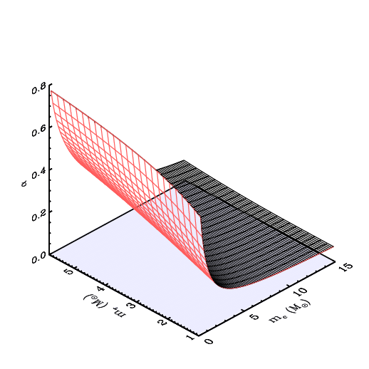
The remnant mass is a function of the initial stellar mass , which may be approximated by a simple power-law, , where is a constant. Using the remnant masses obtained by van den Hoek & Groenewegen (1997) and Woosley & Weaver (1995) for LIM and high mass (HM) stars, respectively, one obtains and for stellar masses less than (see Fig. 1).
The lock-up fraction , used in the model equations discussed in Sect. 2.3, is obtained as . Adopting an IMF of the form shown above in Eq. (22) and defining , where is the incomplete gamma-function, one arrives at the expression (which holds for , )
| (15) |
where , and is the minimum stellar mass effectively contributing to the matter cycle at the considered redshift. With the parameter values given in Table 1 and (the initial mass for which the stellar lifetime corresponds to the typical age of galaxies at ) the lock-up fraction for a normal Larson (1998) IMF () becomes , and in the top-heavy () case . As shown in the right panel of Fig. 1, is a steep function of the turn-over mass , but only weakly dependent on . Hence, the choice of is not critical for either , nor the effective primary yield .
Gall (2010) computed the total dust productivity of a generation of stars considering different IMFs and stellar dust-production efficiencies, . Accordig to Gall (2010) the dust production efficiency derived from observations of SN remnants is well-approximated by a power law, which connects nicely with theoretically expected efficiencies for AGB stars (Ferrarotti & Gail, 2006). If this is a general law for stellar dust production, SNe are insignificant dust producers when weighted by an IMF. Theoretical work, as well as a handfull of observational studies, allows for a much higher efficiency in SNe. Using the results of Todini & Ferrara (2001), Gall (2010) find that AGB stars would be insignificant relative to SNe as dust producers if no dust destruction of SN-formed dust occur due to the reverse shock.
The integrated (IMF-weighted) yields calculated by Gall (2010) is used in this paper, i.e., three cases are considered (see Table 2): ’observed’ SN dust yields, theoretical SN yields with dust destruction due to reverse shocks (Bianchi & Schneider, 2007, ’high’ yield,), and the theoretical ’upper limit’ according to Todini & Ferrara (2001, referred to as ’maximal’ yield) – all three in combination with the theoretical results for AGB stars (Ferrarotti & Gail, 2006; Zhukovska, Gail & Trieloff, 2008).
| IMF | |||
|---|---|---|---|
| Normal | |||
| Top-heavy |
2.5 Evolution of the dust-to-gas ratio
2.5.1 Closed-box evolution
A ’closed-box’ evolution is obviously incompatible with the scenario described above in Sect. 2.1. But for completenes, and since it corresponds to the scenario studied by Valiante et al. (2009) as well as Gall et al. (2010b), it is included also here. If there is no infall, the rate of change of stellar mass is
| (16) |
Assuming no dust destruction, combination of Eq. (16) and Eq. (10) gives the classical closed-box solution,
| (17) |
Replacing with the metal yield , this is also the solution for the metallicity in a closed-box scenario. If the dust-destruction term is included, the solution reads (Edmunds, 2001; Dwek et al., 2007),
| (18) |
This solution differs from the classical closed-box soultion in that as . Assuming that dust grains may form and grow out of metals produced by previous generations of stars, i.e., a kind of ’secondary’ dust, one may redefine the dust yield as
| (19) |
where is the fraction of the metals present in the ISM that will form dust grains. There is a natural upper limit to the value of since , i.e., the dust mass cannot exceed the total mass of metals available.
With the modification above, the solution for becomes (Edmunds, 2001, see also)
| (20) |
where . For the special case (no dust destruction) the solution is
| (21) |
2.5.2 Galaxy formation by infall
Assume the rate of gas consumption is exactly balanced by the rate of infall. With this assumption made, and no dust destruction term, the solution to Eq. (10) is the ’extreme infall model’ by Larson (1972), i.e.,
| (22) |
Adding dust destruction, the solution for has the same mathematical form as the Larson (1972) solution, but with an extra parameter ,
| (23) |
which reduces to Eq. (22) if (). Using the modified yield introduced in Eq. (19) the solution for becomes
| (24) |
where is defined as before, for the closed-box case. For the special case (no dust destruction) the solution is
| (25) |
2.5.3 Evolved systems
Even high- galaxies may have quite evolved stellar populations, e.g., they may be in (or approaching) a ’post-starburst state’ after an intense initial episode of star formation. One should note that the dust-to-gas ratio in the solutions above can never decrease (although can) since is always positive. Hence, it is of interest to know whether is approaching a constant value and thus has an upper limit or not.
For a closed-box scenario without dust destruction by SNe (), as . Including dust destruction (), there is an upper limit since then as , given that is treated as constant. Including ’secondary’ dust production, since the second terms of Eqs. (20) and (21) are simple functions the closed-box solution without dust destruction, which are monotonically increasing.
Any infall model where the rate of infall is proportional to the star-formation rate - not only the Larson (1972) model - has always an upper limit to . In Larson’s extreme infall model the metallicity can never exceed the yield. A similar upper limit exists also for a dust evolution model with infall, although the limit may be lower due to dust destruction. The dust-to-gas ratio will rapidly reach a constant value, i.e., as if no dust destruction by SNe is present, and if it is. With the ’secondary’ dust included, again approaches a constant value, this time given by
| (26) |
To sum up, has (within the present framework) an upper limit with only two exceptions:
- 1.
a closed box without any dust destruction,
- 2.
a closed box with ’seconday’ dust production.
Since a real galaxy cannot strictly be a ’closed box’, it is fair to assume that there is an upper limit to the gas-to-dust ratio in most cases.
2.6 Evolution of the dust-to-metals ratio
A constant dust-to-metals ratio , is commonly adopted in models of galactic evolution (Edmunds & Eales, 1998; Pei et al., 1999, e.g.). From observations, the dust-to-metals ratio is known to be essentially constant in the local Universe (Issa et al., 1990), while a lower (but similar) ratio is found at somewhat higher redshift (Vladilo, 1998, see, e.g.). Edmunds & Eales (1998) considered a simplistic model where was fixed, but it was later shown by Edmunds (2001) that could, at least in principle, vary significantly over time. However, the -evolution approaches a constant value in many cases, so for evolved galaxies of similar type one may expect an approximately universal .
From Eqs. (18-25) it is evident that the dust-to-gas ratio for the different models can be expressed as functions of the metallicity . Hence, for a closed-box
| (27) |
and for the extreme infall case,
| (28) |
From the equations above it is obvious that the evolution of leads to different ’end-states’ depending on the assumptions made for each model. may thus reach a constant value, but can also grow without bound or approach zero as a galaxy evolves.
Since very high dust-to-metals ratios are not observed at any redshift (but see, e.g. Galliano et al., 2003; Vladilo, 2004, for examples of variations), it seems the closed-box case with and ’secondary’ non-stellar dust production is less likely, or star formation has to essentially cease at some point. It also appears that either the dust yield must be a significan fraction of the metal yield, or non-stellar ’secondary’ dust production must play an important role in the local as well as the high- Universe. For the Milky Way , which is roughly the ratio found in most local galaxies of similar type (Issa et al., 1990, see, e.g.), and DLAs at also show similar ratios (Vladilo, 1998).


3 Results and Discussion
Valiante et al. (2009) have suggested that stellar production of dust (in SNe and AGB stars) is high enough to explain the dust-mass estimates of quasar host galaxies at high , in particular the host galaxy of SDSS J1148+525. But is this true under all circumstances? Michalowski et al. (2010b) have shown that the minimal yield needed to explain the observationally inferred dust masses in sub-millimeter galaxies at is per SN if the observational constraints on the stellar and gas mass are assumed to be correct. Their result is marginally consistent with the theoretical maximum obtained by Todini & Ferrara (2001), but does not account for any type of dust destruction.
The main result of the present paper is that only the most extreme, but also less likely, scenarios for cosmic dust production can reproduce the dust masses inferred from observations of high- galaxies. That is a scenario which requires essentially no dust destruction - neither due to the reverse shock in SN-explosions nor in the ISM due to kinetic energy injection by SNe - and extensive non-stellar dust production seems necessary.
Another important result is that galaxy formation by merger events (and accretion of pristine gas), i.e., a cosmologically motivated rate of infall, slows down the build-up of the interstellar dust component quite significantly. This is partly due to the trivial fact that the ISM is diluted from the unenriched gas falling into the galaxy, but also the fact that an infall scenario typically leads to significantly shorter dust destruction time scales (see Fig. 5).
3.1 Comparison with observed properties of high- galaxies
It is reasonable to restrict a general comparison with observations to constraints derived for the infall scenario, since in the current paradaign for galaxy formation galaxies are formed through mass assembly. Furthermore, it can be assumed that dust rich high- galaxies are, despite their redshifts, in a relatively evolved state where a large fraction of the baryonic mass is stars, i.e., the time scale for their assembly short. A good starting point is therefore Eq. (26) in Sect. 2.5.2.
Using Eq. (26) with one can obtain upper limits to the dust masses possible in an evolved system for a given dust yield and efficiency of ’secondary’ dust production. With as the allowed range, Eq. (26) constrains the possible regions in the dust/gas-plane for given yields. In Fig. 2 evolved infall models with ’secondary’ dust production (but without dust destruction) are compared to observationally inferred dust masses of high- galaxies (Michalowski et al., 2010a; Michalowski et al., 2010b) and local galaxies (Devereux & Young, 1990).
The light-blue region (grey in printed version) is only accessible using the ’observed’ yield and the darker blue/grey region can only be reached using the theoretical ’maximum’ yield according to Todini & Ferrara (2001). The overlapping (hatched) region is accessible using either one of the ’high’ and ’maximum’ yield depending on the amount of ’secondary’ dust production. The dust content of the galaxies with the highest dust-to-gas ratios can only be explained with the theoretical ’maximum’ yield in combination with a relatively large . This will be discussed in more detail below. Note that the gas mass for the high- galaxies are taken to be twice the observed H2-mass to account for a neutral gas component, which cannot be detected in these objects (McGreer et al., 2011, the fraction of neutral gas has been estimated to be , see).

As can be seen in Fig. 2, the dust-to-gas ratios of high- galaxies are quite remarkable. Half of the sample considered here have , i.e., larger than the total metallicity of the solar neighbourhood. One may argue that this fact implies gas masses which are about one order of magnitude larger than those obtained through observational estimates of the molecular gas (Gall et al., 2010b, see also models by). However, the uncertainties associated with the gas mass are certainly not on an order of magnitude scale. In fact, the total gas mass is not likely to be more than roughly a factor 2 larger if atomic hydrogen and helium is added, and the uncertainty in the conversion factor between CO and H2 () can at most be a few times larger than the value commonly used for high- objects. A value around is normally used for high- quasars (Downes & Solomon, 1998, see, e.g.), while for local spiral galaxies , is typically taken to be (Solomon & Barrett, 1991, see, e.g.). For local starburst galaxies , however.
It seems non-stellar dust production/growth may be required to reproduce the high dust-to-gas ratios. Dust may grow in dense molecular clouds in the ISM through accretion onto seed particles (most likely originating from stars) given enough time (Draine, 1990). This component may be significant, possibly a more important contribution than dust grown in stellar atmospheres and SN remnamts (Zhukovska, Gail & Trieloff, 2008; Asano et al., 2010). Furthermore, Elvis et al. (2002) have suggested dust may be nucleated (and grow) in broad emission line clouds in outflowing quasar winds. Both processes (growth in the ISM and formation in quasar winds) can be indirectly associated with star formation. Stars form primarely in dense molecular clouds which is also where dust grains in the ISM may grow through accretion. Quasar-wind outflow rates can be considered roughly proportional to the mass of the supermassive black hole (see Pipino et al., 2011, references therein) and are thus linked to the star formation rate (or growth of the stellar mass) assuming that the black hole is growing due to the galactic mass assembly (DeBuhr et al., 2010; Sarria et al., 2010). Hence, the non-stellar dust production/growth may effectively be modelled by introducing a modified (metallicity-dependent) yield as in Eq. (19). The possibility of grains forming in quasar ourflows and grains growing in the ISM should be investigated further by more detailed modelling before one concludes that this is the solution to the dust formation problem in the early Universe, however.
Although significant non-stellar dust production is an attractive idea, much of the dust production problem at high can be resolved by assuming the true gas mass may be a few times higher due to a significant atomic component and uncertainties in the derivation of the molecular component (see above), combined with the fact that dust masses are hard to quantify with high precision. It may very well be that the dust masses derived for, e.g., high- quasars are too large due to the fact that the model for the dust emission is quite rudimentary. Dust mass estimates are generally uncertain up to a factor of a few (Silva et al., 1998). Hence, the true dust-to-gas ratio could, at least in principle, be an order of magnitude lower, which could then be explained by stellar dust production alone. If is only a few times , the required dust yield is reasonable from a theoretical point of view (c.f. the effect of reverse shocks) and consistent with results for local galaxies (see Fig. 2).
3.2 SDSS J1148+525
The host galaxy of the SDSS J1148+5251 quasar has received considerable attention in the literature since it appears to have an unexpectedly large dust mass for its high redshift (), which seems to require a rather dramatic early star formation history if dust is mainly produced in stars (Dwek et al., 2007; Valiante et al., 2009; Gall et al., 2010b; Pipino et al., 2011, see, e.g., the models by). This quasar host galaxy is used as a test bench also in the present paper. SDSS J1148+525 provides insight on the evolutionary states of dust-rich quasar hosts at high redshifts.
Massive high- galaxies seem to have reached a relatively evolvled state, despite their high redshifts, indicating that they form in a rapid series of mergers/infall events as in the model by Li et al. (2007). The time scale of the build-up of the stellar mass is clearly not more than a few Myr. As a consequence, they have typically reached solar, or even supersolar, metallicities and the subsequent evolution (from the observed state until present time) will neither change the metallicity, nor the dust-to-gas ratio dramatically.
The age of the Universe at in the standard CDM model is Myr and galaxy formation is here assumed to start at corresponding to Myr. The host galaxy of SDSS J1148+5251 has in such case evolved for 550 Myr prior to its observed state. Li et al. (2007) constructed a merger tree, extracted from a cosmological simulation, to follow the hierarchical mass assembly of a galaxy thought to be similar to the host galaxy of SDSS J1148+5251. Here, just as in the work by Valiante et al. (2009), their resultant star-formation history (SFH) is used as input (see Fig. 3). In practice, however, the quantity used is the time-integrated star-formation rate, i.e., the stellar mass,
| (29) |
which was computed numerically from the data shown in Fig. 3 using a simple Romberg routine. In contrast to Valiante et al. (2009), a scaled-down version of this SFH is considered to meet observational constraints on the total mass.
Using the analytic model described in Sect. 2.3, 150 parameter configurations are considered (see Appendix A) in order to find the most likely models given some observational constraints to the dust mass in SDSS J1148+5251 (see Valiante et al., 2009, and references therein) and the dust-to-metals ratios found in damped Ly absorbers at lower redshifts (Vladilo, 1998, ). Although inconsistent with a merger scenario, the closed-box case is here considered because (1) previous studies (Valiante et al., 2009; Gall et al., 2010b) have considered the SDSS J1148+5251 quasar host galaxy to be a ’closed box’, (2) it is important to analyse the net differeces between an infall and closed-box scenario, since the evolution of the gas mass affects net dust-destruction efficiency (see Eq. 5) and (3) infall always lowers the efficiency of metal production (Edmunds, 1990).


| Models | [] | [] | [] | IMF |
|---|---|---|---|---|
| 1-30 | 0, 100, 200, 1000 | Normal | ||
| 31-60 | 0, 20, 100, 200 | Top-heavy | ||
| 61-90 | 0, 100, 200, 1000 | Normal | ||
| 91-120 | 0, 100, 200, 1000 | Normal | ||
| 121-150 | 0, 20, 100, 200 | Top-heavy |
Only a few of the 150 models seem to reproduce both the expected dust mass and a reasonable dust-to-metals ratio (the models presented in Fig. 4). A plausible dust-mass range for the SDSS J1148+525 host is that adopted by Valiante et al. (2009), i.e., . Given the spread and uncertainty of the dust masses obtained by different authors (see Valiante et al., 2009, and references therein), a dust mass in the range is here considered to be consistent with the observations. A ’reasonable’ range for the dust-to-metals ratio is here taken to be the same as for the sample of DLAs at medium high redshift studied by Vladilo (1998), as is not changing much after the intial phase of galaxy evolution unless the grain-growth rate is particularly low (see, e.g. Edmunds, 2001, Fig. 4). Assuming dust of Galactic type, the DLAs considered by Vladilo (1998) places this quantity between 42% and 89% (typically 60%) of the Galactic value, where the latter is (Meyer et al., 1998; Whittet, 1991).
The grid of models can be divided into five sub-sets of models based on the assumptions made regarding total mass, stellar mass, gas mass (at ), dust destruction and the IMF (see Tables 1 and 3). The first sub-set (models 1-30) represents an attempt to reprouce the metals and dust assuming the star formation builds up to roughly the same stellar mass as in the simulation by Li et al. (2007), while still maintaining the lower-limit gas mass suggested by observations. With model 11 as the only exception, non-stellar dust production appears necessary to reach above of dust at . A few models (6, 12 and 26) do reach above and may be considered marginally consistent with observations in that regard. Model 26 is the only infall model without non-stellar dust production (among models 1-30) which is consistent with the dust mass derived from observations (see Fig. 4). It is also consistent with the range of dust-to-metals ratios one would expect for a galaxy like SDSS J1148+525 (see Fig. 6).
Changing the IMF from a normal Larson (1998) IMF () to at top-heavy ditto () increases both the amount of dust production as well as the dust destruction by SN shocks, as can be seen from models 31-60. Models 36, 42, 51 and 57 are all reproducing the expected range for the dust mass, while all models with higher dust destruction efficiency () predict too much dust destruction due to the significantly increased SN-rate. The resultant dust masses are in those cases at most a few times . Models 31-60 are essentially ruled out because the resultant metallicities are too high to be realistic ( at ) and inconsistent with the expected range of dust-to-metals ratios (see Fig. 6).
Models 61-90 (see Fig. 6, and Table 6) are analogous to the numerical model by Valiante et al. (2009) in that they have similar stellar and gas masses (a total baryon mass of ) and represent a closed-box scenario. The stellar dust yield referred to as the ’high’ yield (see Table 2) and corresponds to the model preffered by Valiante et al. (2009). The resultant gas mass () is significantly higher than the mass inferred from observations (Walter et al., 2004, see, e.g.). With this high gas mass, even the low (’observed’) dust yield (Gall et al., 2010b, see) is sufficient to reproduce the observed dust mass, and the ’maximal’ yield leads to an over-production of dust in several cases (models 71-73 and 86-88). This is the main reason why the model by Valiante et al. (2009) is marginally consistent with the high dust mass derived from observations without invoking dust growth in the ISM or any other seconday dust source. More gas simply means more dust without resulting in unrealistic dust-to-gas ratios. But as one can see in Fig. 6, the total amount of metals is generally too high to have dust-to-metals ratios in the expected range.
Applying observational constraints on both the gas mass and the stellar mass (models 91-120) results in two plausible models. Both are models without dust destruction in the ISM and the ’maximal’ stellar yield (see Table 2). Adding non-stellar dust production (as it is implemeted here) means no actual improvement for the models with lower yields. It essentially requires that all metals in the ISM are turned into dust.
Adding a top-heavy IMF (models 121-150, see Fig. 11) leads to a result very similar to that of models 31-60 (also with a top-heavy IMF), i.e., the over-all metal production is not sufficient to reproduce the expected range of dust to metals.
3.3 Infall vs. closed box
Among the seven models of SDSS J1148+525 that reproduce the expected dust mass and dust-to-metals ratio (see previous section), only two are infall models. One may note as well that all the closed-box models presented here (Valiante et al., 2009, and the model by) are conceptually inconsistent, since Li et al. (2007) consider a galaxy being formed by a sequence of merger events, where the smaller progenitor galaxies are very metal poor and have had very little star formation (). The infall models (16-30, 46-60, 76-90, 106-120 and 136-150) are therefore more appropriate. This fact was indeed acknowledged by Valiante et al. (2009), although the exact consequences were not discussed.
From the present study it is clear, however, that infall models are not preferred over closed-box models in that they do not reproduce the dust mass and/or overall metallicity better than closed-box models. Infact, a merger/infall scenario requires a higher stellar dust yield in order to produce the same dust mass, which is due to the effects of the dilution by pristine infall (Edmunds, 1990, see, e.g.) and the fact that the dust destruction time scale is proportional to gas mass. The latter is important during the early phase of evolution, since in a closed-box scenario the initial gas mass is always equal to the total mass of baryons. The gas mass is never as high as during the initial phase of the gas mass evolution, which means that the dust destruction time scale is significantly longer at early times (when the rate of dust production is at its highest) compared to the infall scenario (see Eq. 5 and the example in Fig. 5).
In the model of SDSS J1148+525, the intense star formation expected during the first 400 Myr would produce a lot of stellar dust, while would still be relatively long on average in the closed-box case. As a consequence, the effective dust production have to be higher. If an infall scenario is adopted, the gas mass during the early evolution is lower even if the final total mass of baryons is the same. For example, in models 1-30 the dust destruction time scale is about 15 times shorter for infall models compared to closed-box models and therefore infall models have a lower dust-formation efficiency.
Infall models always require a larger metal yield than the closed-box models in order to contain the same amount metals. As discussed above, the dust-to-metals ratio should be roughly that of DLAs (Vladilo, 1998). The lower net-production of dust for a given stellar mass of infall models tends to result in higher -values (see Fig. 6). The infall models presented here are perhaps unrealistic in that they assume all gas ejected by evolved stars and all infalling gas is converted into new stars (keeping ). But the dust yield required to produce the estimated dust mass is at the high end and the star-formation efficiency will under all circumstances be high in quasar host galaxies at high redshifts.
3.4 Quasar outflows
As argued in Sect. 2.2, the presence of a galactic wind driven by SNe will have roughly the same effect on the dust mass as dust destruction by SNe has, thus making it even harder to obtain the high dust masses in some high- galaxies. However, the outflows associated with quasars may also have a totally different effect. Elvis et al. (2002) suggested that dust may be created in broad emission line clouds associated with quasar outflows. As opposed to the gas in the ISM, these gas clouds could in principle (remains to be proven) have both nucleation and growth of dust grains. This fact makes quasar outflows a possible source for the ’missing dust’ in models of dust formation in high- quasar host galaxies. The models presented here suggest the efficiency of dust production must be quite high, i.e., a large fraction of the atomic metals in the gas must be converted into dust (essentially all the metals in the galaxy need to be in dust in many cases, see tables in Appendix A). This might be a problem, since one can only have as much metals as can be produced by the stars and the total gas mass in a quasar outflow is not likely to be very large. Thus quasar outflows may contribute, but the contribution can be considered negligible (Pipino et al., 2011, see also modelling results by).

3.5 A top-heavy IMF?
There is a variety of evidence for top-heavy IMFs in starburst environments (Dabringhausen et al., 2009, see, e.g.,). Valiante et al. (2009) showed that in their model LIM stars contributed about 80% of the dust, using a Larson (1998) IMF, which is similiar to that of Salpeter (1955) except at low masses where the Larson (1998) IMF has a smooth turn-over. But with a top-heavy IMF the situation is quite different.
From observations it seems LIM stars are producing significantly more dust per stellar mass than HM stars (cf. the ’observed’ yield in Table 2). Hence, a top-heavy IMF would under these circumstances result in a lower total stellar dust yield . If the dust production is dominated by HM stars, on the other hand, a top-heavy IMF leads to a significantly increased dust production (Gall et al., 2010b). However, a larger fraction of HM stars also increases the SN-rate, which in turn leads to more interstellar dust destruction due to SN-shocks (see Sect. 3.2, Fig. 6, Models 31-60 and 121-150 in Appendix A). But if this type of dust destruction is negligible, an initially top-heavy IMF may help to boost dust production in the early Universe. In general, though, a top-heavy IMF means no particular improvment since (1) dust destruction due SN-shocks is expected and (2) the dust-to-metals ratio changes in an unfavourable direction (again, see Fig. 6, where it is clear that the ratios are too low).


4 Summary and Conclusions
Stars can only produce a limited amount of dust and the time-scale of survival of dust in the ISM may not be long enough. Thus, there are three fundamental reasons why stellar sources probably cannot explain the dust masses observed at several high- objects:
- 1.
Stellar yields must under most circumstances be close to the theoretical maximum for simple dust evolution models to be consistent with dust masses derived from observations.
- 2.
A top-heavy IMF means no paricular improvement since the SN-rate increases and therefore the rate of dust destruction increases as well. Consequently the dust-to-metals ratio changes in an unfarvourable fashion.
- 3.
Infall of gas (which is more likely than a closed-box scenario) may shorten the dust-destruction time scale and therby lower the effective stellar dust production.
The simple analytical models presented in this paper suggest the dust-mass problem in high- galaxies cannot be solved by only adding the contribution from AGB stars. The inclusion of AGB stars by made Valiante et al. (2009) adds new and important information, but it does not provide a complete and viable solution to the dust production problem at high redshifts.
Elvis et al. (2002) have suggested dust may be created in broad emission line clouds in an outflowing quasar wind. One may also assume dust grains can form, or at least grow, in the interstellar gas of quasar host galaxies. However, neither hypotheses can properly solve the dust production problem, because the amount of metals needed as raw-material for dust formation cannot be produced by stars alone in many cases.
There is essentially only two ways out of the dilemma described above, is either significant non-stellar dust production (e.g., growth of dust grains in the ISM or dust formation associated with quasar outflows) or signifiant systematic errors in the dust and (molecular) gas masses derived from observations. In a few cases it may be sufficient to assume no dust destruction, but this cannot solve the problem in general.
Acknowledgments
The reviewer, Mike Edmunds, is thanked for his valuable comments which helped to improve the paper. Anja C. Andersen and Christa Gall are thanked for interesting discussions on dust in the early Universe and comments on the contents of this paper. Rosa Valiante is thanked for providing the input data of her model of SDSS J1148+525. The author acknowledges support from Vetenskapsrådet (the Swedish Research Council). The Dark Cosmology Centre is funded by the Danish National Research Foundation.
References
- Asano et al. (2010) Asano R.S, Takeuchi T.T., Hirashita H. & Inoue A.K., 2010, A&A, submitted
- Barlow et al. (2010) Barlow, M. J., Krause, O., Swinyard, B. M., et al. 2010, A&A, 519, L138
- Beelen et al. (2006) Beelen, A., Cox, P., Benford, D. J., et al. 2006, ApJ, 642, 694
- Bertoldi et al. (2003) Bertoldi F. et al., 2003, A&A 406, L55
- Bianchi & Schneider (2007) Bianchi S. & Schneider R., 2007, MNRAS 378, 973
- Dabringhausen et al. (2009) Dabringhausen J., Kroupa P. & Baumgardt H., 2009, MNRAS, 395, 1529
- DeBuhr et al. (2010) Debuhr J., Quataert E., Ma C.-P. & Hopkins P., 2010, MNRAS, 406, L55
- Devereux & Young (1990) Devereux N.A. & Young J.S., 1990, Apj, 359, 42
- Draine (1990) Draine B., 1990, ASPC, 12, 193
- Downes & Solomon (1998) Downes D. & Solomon P.M., 1998, ApJ, 507, 615
- Dunne et al. (2009) Dunne L., Maddox S. J., Ivison R. J., et al. 2009, MNRAS, 394, 1307
- Dwek et al. (2007) Dwek E., Galliano F. & Jones A.P., 2007, ApJ, 662, 927
- Edmunds (1990) Edmunds M.G., 1990, MNRAS, 246, 678
- Edmunds & Eales (1998) Edmunds M.G. & Eales S.A., 1998, MNRAS, 299, L29
- Edmunds (2001) Edmunds M.G., 2001, MNRAS, 328, 223
- Elvis et al. (2002) Elvis M., Marengo M., Karovska M., 2002, ApJ, 567, L107
- Ferrarotti & Gail (2006) Ferrarotti A.S. & Gail H.-P., 2006, A&A, 447, 553
- Gall (2010) Gall C., 2010, Phd Thesis, Univ. of Copenhagen
- Gall et al. (2010b) Gall C. Andersen A.C. & Hjort J., 2010b, A&A, accepted
- Galliano et al. (2003) Galliano F., Madden S.C., Jones A.P., Wilson C.D., Bernard J.-P. & Le Peintre F., 2003, A&A, 407, 159
- Genzel et al. (2003) Genzel R., Baker A.J., Tacconi L.J., Lutz D., Cox P., Guilloteau S. & Omont A., Apj, 458, 633
- Gomez et al. (2009) Gomez, H. L., Dunne, L., Ivison, R. J., et al. 2009, MNRAS, 397, 1621
- Gomez et al. (2010) Gomez, H. L., Vlahakis, C., Stretch, C. M., et al. 2010, MNRAS, 401, L48
- Grøn (2002) Grøn, Ø., 2002, Eur. J. Phys., 23, 135
- van den Hoek & Groenewegen (1997) van den Hoek L.B. & Groenewegen M.A.T., 1997, A&As, 123, 305
- Issa et al. (1990) Issa M.R., MacLaren I. & Wolfendale A.W., 1990, A&A, 236, 237
- Jiang et al. (2006) Jiang, L., Fan, X., Hines, D. C., et al. 2006, AJ, 132, 2127
- Jiang et al. (2010) Jiang L., Fan X., Brandt W.N., et al., 2010, Nature, 464, 380
- Kotak et al. (2006) Kotak R., Meikle P., Pozzo M., et al., 2006, ApJ, 651, L117
- Kotak et al. (2009) Kotak R., Meikle W.P.S., Farrah D., et al., 2009, ApJ, 704, 306
- Larson (1972) Larson R., 1972, Nature Phys. Sci., 236, 7
- Larson (1998) Larson R., 1998, MNRAS, 301, 569
- Ledoux et al. (2002) Ledoux C., Bergeron J. & Petitjean P., 2002, A&A, 385, 802
- Li et al. (2007) Li Y. et al., 2007, ApJ, 665, 187
- Matsuoka et al. (2009) Matsuoka K., Nagao T., Maiolino R., Marconi A. & Taniguchi Y., 2009, A&A, submitted (arXiv:0905.1581)
- Maiolino et al. (2004) Maiolino R. et al., 2004, Nature, 431, 533
- McGreer et al. (2011) McGreer I.D., Mesinger A., & Fan X., 2011, MNRAS, accepted (arXiv:1101.3314)
- Meikle et al. (2007) Meikle W.P.S. et al., 2007, ApJ, 665, 608
- Meyer et al. (1998) Meyer D.M., Jura M. & Cardelli J.A., 1998, ApJ, 493, 222
- Michalowski et al. (2008) Michalowski M. et al., 2008, ApJ, 672, 817
- Michalowski et al. (2010a) Michalowski M., Watson D. & Hjorth J., 2010, ApJ, 712, 942
- Michalowski et al. (2010b) Michalowski M., Murphy E.J., Hjorth J., Watson D., Gall C. & Dunlop J.S., 2010, A&A, 522, 15
- Morgan & Edmunds (2003) Morgan, H.L. & Edmunds, M.G. 2003, MNRAS, 343, 427
- Morgan et al. (2003) Morgan H.L., Dunne L., Eales S.A., Ivison R.J., Edmunds M.G., 2003, ApJ, 597, L33
- Nozawa et al. (2003) Nozawa T., Kozasa T., Umeda H., Maeda K., & Nomoto K., 2003, ApJ, 598, 78
- Nozawa et al. (2008) Nozawa T., Kozasa T., Tominaga N., et al. 2008, ApJ, 684, 1343
- Pagel (1997) Pagel B.E.J., 1997, ”Nucleosynthesis and Chemical Evolution of Galaxies”, Cambridge Univ. Press
- Pei et al. (1999) Pei Y.C., Fall M. & Hauser M., 1999, ApJ, 522, 604
- Pipino et al. (2011) Pipino A., Fan X.L., Matteucci F., et al., 2011, A&A, 525, 61
- Robson et al. (2004) Robson, I., Priddey, R. S., Isaak, K. G., & McMahon, R. G. 2004, MNRAS, 351, L29
- Salpeter (1955) Salpeter E.E., 1955, ApJ, 121, 161
- Sarria et al. (2010) Sarria J.E., Maiolino R., La Franca F., et al., 2010, A&A, 522,L3
- Silva et al. (1998) Silva L., Granato G. L., Bressan A., & Danese L., 1998, ApJ, 509, 103
- Solomon & Barrett (1991) Solomon P.M. & Barrett J.W., IAUS, 146, 235
- Stanway et al. (2011) Stanway, E.R., Bremer, M.N., Tanvir, N.R., Levan, A.J., Davies & Luke J.M., 2011, to appear in MNRAS.
- Todini & Ferrara (2001) Todini P. & Ferrara A., 2001, MNRAS 325, 726
- Valiante et al. (2009) Valiante R., Schneider R., Bianchi S. & Andersen A.C., 2009, MNRAS, 397, 1661
- Vestergaard (2004) Vestergaard M., ApJ, 601, 676
- Vladilo (1998) Vladilo G., 1998, ApJ, 493, 583
- Vladilo (2004) Vladilo G., 2004, A&A, 421, 479
- Walter et al. (2004) Walter F., Carilli C., Bertoldi F., Menten K., Cox P., Lo K.Y., Fan X. & Strauss M.A., 2004, ApJ, 615, L17
- Whittet (1991) Whittet D.C.B., 1991, Dust in the Galactic Environment, IOP Publishing, Bristol
- Woosley & Weaver (1995) Woosley S.E., Weaver T.A., 1995, ApJS, 101, 181
- Zhukovska, Gail & Trieloff (2008) Zhukovska S., Gail H.-P. & Trieloff M., 2008, A&A, 479, 453
Appendix A Models of SDSS J1148+525
| Model | [] | [] | [] | Description | ||||||
|---|---|---|---|---|---|---|---|---|---|---|
| 1 | 0.63 | - | 0 | 0.00 | - | Closed box, no dust destruction. | ||||
| 2 | 0.63 | - | 100 | 1.00 | 1.59 | Closed box. | ||||
| 3 | 0.63 | - | 200 | 2.00 | 3.17 | Closed box. | ||||
| 4 | 0.63 | - | 1000 | 10.0 | 15.9 | Closed box. | ||||
| 5 | 0.63 | 0.35 | 0 | 0.00 | - | Closed box, ’secondary dust’. | ||||
| 6 | 0.63 | - | 0 | 0.00 | - | Closed box, no dust destruction. | ||||
| 7 | 0.63 | - | 100 | 1.00 | 1.59 | Closed box. | ||||
| 8 | 0.63 | - | 200 | 2.00 | 3.17 | Closed box. | ||||
| 9 | 0.63 | - | 1000 | 10.0 | 15.9 | Closed box. | ||||
| 10 | 0.63 | 0.30 | 0 | 0.00 | - | Closed box, ’secondary dust’. | ||||
| 11 | 0.63 | - | 0 | 0.00 | - | Closed box, no dust destruction. | ||||
| 12 | 0.63 | - | 100 | 1.00 | 1.59 | Closed box. | ||||
| 13 | 0.63 | - | 200 | 2.00 | 3.17 | Closed box. | ||||
| 14 | 0.63 | - | 1000 | 10.0 | 15.9 | Closed box. | ||||
| 15 | 0.63 | 0.30 | 100 | 1.00 | 1.59 | Closed box, ’secondary dust’. | ||||
| 16 | 0.63 | - | 0 | 0.00 | - | Infall, no dust destruction. | ||||
| 17 | 0.63 | - | 100 | 1.00 | 1.59 | Infall | ||||
| 18 | 0.63 | - | 200 | 2.00 | 3.17 | Infall | ||||
| 19 | 0.63 | - | 1000 | 10.0 | 15.9 | Infall | ||||
| 20 | 0.63 | 0.85 | 0 | 0.00 | - | Infall, ’secondary dust’. | ||||
| 21 | 0.63 | - | 0 | 0.00 | - | Infall, no dust destruction. | ||||
| 22 | 0.63 | - | 100 | 1.00 | 1.59 | Infall | ||||
| 23 | 0.63 | - | 200 | 2.00 | 3.17 | Infall | ||||
| 24 | 0.63 | - | 1000 | 10.0 | 15.9 | Infall | ||||
| 25 | 0.63 | 0.80 | 0 | 0.00 | - | Infall, ’secondary dust’. | ||||
| 26 | 0.63 | - | 0 | 0.00 | - | Infall, no dust destruction. | ||||
| 27 | 0.63 | - | 100 | 1.00 | 1.59 | Infall | ||||
| 28 | 0.63 | - | 200 | 2.00 | 3.17 | Infall | ||||
| 29 | 0.63 | - | 1000 | 10.0 | 15.9 | Infall | ||||
| 30 | 0.63 | 0.50 | 0 | 0.00 | - | Infall, ’secondary dust’. |


| Model | [] | [] | [] | Description | ||||||
|---|---|---|---|---|---|---|---|---|---|---|
| 31 | 0.10 | - | 0 | 0.00 | - | Closed box, no dust destruction. | ||||
| 32 | 0.10 | - | 20 | 1.32 | 1.59 | Closed box. | ||||
| 33 | 0.10 | - | 100 | 6.60 | 3.17 | Closed box. | ||||
| 34 | 0.10 | - | 200 | 13.2 | 15.9 | Closed box. | ||||
| 35 | 0.10 | 0.25 | 20 | 1.32 | - | Closed box, ’secondary dust’. | ||||
| 36 | 0.10 | - | 0 | 0.00 | - | Closed box, no dust destruction. | ||||
| 37 | 0.10 | - | 20 | 1.32 | 1.59 | Closed box. | ||||
| 38 | 0.10 | - | 100 | 6.60 | 3.17 | Closed box. | ||||
| 39 | 0.10 | - | 200 | 13.2 | 15.9 | Closed box. | ||||
| 40 | 0.10 | 0.25 | 20 | 1.32 | - | Closed box, ’secondary dust’. | ||||
| 41 | 0.10 | - | 0 | 0.00 | - | Closed box, no dust destruction. | ||||
| 42 | 0.10 | - | 20 | 1.32 | 1.59 | Closed box. | ||||
| 43 | 0.10 | - | 100 | 6.60 | 3.17 | Closed box. | ||||
| 44 | 0.10 | - | 200 | 13.2 | 15.9 | Closed box. | ||||
| 45 | 0.10 | 0.12 | 20 | 1.32 | 1.59 | Closed box, ’secondary dust’. | ||||
| 46 | 0.10 | - | 0 | 0.00 | - | Infall, no dust destruction. | ||||
| 47 | 0.10 | - | 20 | 1.32 | 1.59 | Infall | ||||
| 48 | 0.10 | - | 100 | 6.60 | 3.17 | Infall | ||||
| 49 | 0.10 | - | 200 | 13.2 | 15.9 | Infall | ||||
| 50 | 0.10 | 0.55 | 20 | 1.32 | - | Infall, ’secondary dust’. | ||||
| 51 | 0.10 | - | 0 | 0.00 | - | Infall, no dust destruction. | ||||
| 52 | 0.10 | - | 20 | 1.32 | 1.59 | Infall | ||||
| 53 | 0.10 | - | 100 | 6.60 | 3.17 | Infall | ||||
| 54 | 0.10 | - | 200 | 13.2 | 15.9 | Infall | ||||
| 55 | 0.10 | 0.55 | 20 | 1.32 | - | Infall, ’secondary dust’. | ||||
| 56 | 0.10 | - | 0 | 0.00 | - | Infall, no dust destruction. | ||||
| 57 | 0.10 | - | 20 | 1.32 | 1.59 | Infall | ||||
| 58 | 0.10 | - | 100 | 6.60 | 3.17 | Infall | ||||
| 59 | 0.10 | - | 200 | 13.2 | 15.9 | Infall | ||||
| 60 | 0.10 | 0.30 | 20 | 1.32 | - | Infall, ’secondary dust’. |


| Model | [] | [] | [] | Description | ||||||
|---|---|---|---|---|---|---|---|---|---|---|
| 61 | 0.63 | - | 0 | 0.00 | - | Closed box, no dust destruction. | ||||
| 62 | 0.63 | - | 100 | 1.00 | 1.59 | Closed box. | ||||
| 63 | 0.63 | - | 200 | 2.00 | 3.17 | Closed box. | ||||
| 64 | 0.63 | - | 1000 | 10.0 | 15.9 | Closed box. | ||||
| 65 | 0.63 | 0.05 | 100 | 1.00 | 1.59 | Closed box, ’secondary dust’. | ||||
| 66 | 0.63 | - | 0 | 0.00 | - | Closed box, no dust destruction. | ||||
| 67 | 0.63 | - | 100 | 1.00 | 1.59 | Closed box. | ||||
| 68 | 0.63 | - | 200 | 2.00 | 3.17 | Closed box. | ||||
| 69 | 0.63 | - | 1000 | 10.0 | 15.9 | Closed box. | ||||
| 70 | 0.63 | 0.06 | 200 | 2.00 | 3.17 | Closed box, ’secondary dust’. | ||||
| 71 | 0.63 | - | 0 | 0.00 | - | Closed box, no dust destruction. | ||||
| 72 | 0.63 | - | 100 | 1.00 | 1.59 | Closed box. | ||||
| 73 | 0.63 | - | 200 | 2.00 | 3.17 | Closed box. | ||||
| 74 | 0.63 | - | 1000 | 10.0 | 15.9 | Closed box. | ||||
| 75 | 0.63 | 0.12 | 1000 | 10.0 | 15.9 | Closed box, ’secondary dust’. | ||||
| 76 | 0.63 | - | 0 | 0.00 | - | Infall, no dust destruction. | ||||
| 77 | 0.63 | - | 100 | 1.00 | 1.59 | Infall | ||||
| 78 | 0.63 | - | 200 | 2.00 | 3.17 | Infall | ||||
| 79 | 0.63 | - | 1000 | 10.0 | 15.9 | Infall | ||||
| 80 | 0.63 | 0.12 | 200 | 2.00 | 3.17 | Infall, ’secondary dust’. | ||||
| 81 | 0.63 | - | 0 | 0.00 | - | Infall, no dust destruction. | ||||
| 82 | 0.63 | - | 100 | 1.00 | 1.59 | Infall | ||||
| 83 | 0.63 | - | 200 | 2.00 | 3.17 | Infall | ||||
| 84 | 0.63 | - | 1000 | 10.0 | 15.9 | Infall | ||||
| 85 | 0.63 | 0.10 | 200 | 2.00 | 3.17 | Infall, ’secondary dust’. | ||||
| 86 | 0.63 | - | 0 | 0.00 | - | Infall, no dust destruction. | ||||
| 87 | 0.63 | - | 100 | 1.00 | 1.59 | Infall | ||||
| 88 | 0.63 | - | 200 | 2.00 | 3.17 | Infall | ||||
| 89 | 0.63 | - | 1000 | 10.0 | 15.9 | Infall | ||||
| 90 | 0.63 | 0.20 | 1000 | 10.0 | 15.9 | Infall, ’secondary dust’. |


| Model | [] | [] | [] | Description | ||||||
|---|---|---|---|---|---|---|---|---|---|---|
| 91 | 0.63 | - | 0 | 0.00 | - | Closed box, no dust destruction. | ||||
| 92 | 0.63 | - | 100 | 1.00 | 1.59 | Closed box. | ||||
| 93 | 0.63 | - | 200 | 2.00 | 3.17 | Closed box. | ||||
| 94 | 0.63 | - | 1000 | 10.0 | 15.9 | Closed box. | ||||
| 95 | 0.63 | 1.50 | 0 | 0.00 | - | Closed box, ’secondary dust’. | ||||
| 96 | 0.63 | - | 0 | 0.00 | - | Closed box, no dust destruction. | ||||
| 97 | 0.63 | - | 100 | 1.00 | 1.59 | Closed box. | ||||
| 98 | 0.63 | - | 200 | 2.00 | 3.17 | Closed box. | ||||
| 99 | 0.63 | - | 1000 | 10.0 | 15.9 | Closed box. | ||||
| 100 | 0.63 | 1.50 | 0 | 0.00 | - | Closed box, ’secondary dust’. | ||||
| 101 | 0.63 | - | 0 | 0.00 | - | Closed box, no dust destruction. | ||||
| 102 | 0.63 | - | 100 | 1.00 | 1.59 | Closed box. | ||||
| 103 | 0.63 | - | 200 | 2.00 | 3.17 | Closed box. | ||||
| 104 | 0.63 | - | 1000 | 10.0 | 15.9 | Closed box. | ||||
| 105 | 0.63 | 1.00 | 0 | 0.00 | - | Closed box, ’secondary dust’. | ||||
| 106 | 0.63 | - | 0 | 0.00 | - | Infall, no dust destruction. | ||||
| 107 | 0.63 | - | 100 | 1.00 | 1.59 | Infall | ||||
| 108 | 0.63 | - | 200 | 2.00 | 3.17 | Infall | ||||
| 109 | 0.63 | - | 1000 | 10.0 | 15.9 | Infall | ||||
| 110 | 0.63 | 0.97 | 0 | 0.00 | - | Infall, ’sec. dust’, max. . | ||||
| 111 | 0.63 | - | 0 | 0.00 | - | Infall, no dust destruction. | ||||
| 112 | 0.63 | - | 100 | 1.00 | 1.59 | Infall | ||||
| 113 | 0.63 | - | 200 | 2.00 | 3.17 | Infall | ||||
| 114 | 0.63 | - | 1000 | 10.0 | 15.9 | Infall | ||||
| 115 | 0.63 | 0.95 | 0 | 0.00 | - | Infall, ’sec. dust’, max. . | ||||
| 116 | 0.63 | - | 0 | 0.00 | - | Infall, no dust destruction. | ||||
| 117 | 0.63 | - | 100 | 1.00 | 1.59 | Infall | ||||
| 118 | 0.63 | - | 200 | 2.00 | 3.17 | Infall | ||||
| 119 | 0.63 | - | 1000 | 10.0 | 15.9 | Infall | ||||
| 120 | 0.63 | 0.64 | 0 | 0.00 | - | Infall, ’sec. dust’, max. . |


| Model | [] | [] | [] | Description | ||||||
|---|---|---|---|---|---|---|---|---|---|---|
| 121 | 0.10 | - | 0 | 0.00 | - | Closed box, no dust destruction. | ||||
| 122 | 0.10 | - | 20 | 1.32 | 1.59 | Closed box. | ||||
| 123 | 0.10 | - | 100 | 6.60 | 3.17 | Closed box. | ||||
| 124 | 0.10 | - | 200 | 13.2 | 15.9 | Closed box. | ||||
| 125 | 0.10 | 0.55 | 20 | 1.32 | - | Closed box, ’secondary dust’. | ||||
| 126 | 0.10 | - | 0 | 0.00 | - | Closed box, no dust destruction. | ||||
| 127 | 0.10 | - | 20 | 1.32 | 1.59 | Closed box. | ||||
| 128 | 0.10 | - | 100 | 6.60 | 3.17 | Closed box. | ||||
| 129 | 0.10 | - | 200 | 13.2 | 15.9 | Closed box. | ||||
| 130 | 0.10 | 0.50 | 20 | 1.32 | - | Closed box, ’secondary dust’. | ||||
| 131 | 0.10 | - | 0 | 0.00 | - | Closed box, no dust destruction. | ||||
| 132 | 0.10 | - | 20 | 1.32 | 1.59 | Closed box. | ||||
| 133 | 0.10 | - | 100 | 6.60 | 3.17 | Closed box. | ||||
| 134 | 0.10 | - | 200 | 13.2 | 15.9 | Closed box. | ||||
| 135 | 0.10 | 0.25 | 20 | 1.32 | 1.59 | Closed box, ’secondary dust’. | ||||
| 136 | 0.10 | - | 0 | 0.00 | - | Infall, no dust destruction. | ||||
| 137 | 0.10 | - | 20 | 1.32 | 1.59 | Infall | ||||
| 138 | 0.10 | - | 100 | 6.60 | 3.17 | Infall | ||||
| 139 | 0.10 | - | 200 | 13.2 | 15.9 | Infall | ||||
| 140 | 0.10 | 0.70 | 20 | 1.32 | - | Infall, ’secondary dust’. | ||||
| 141 | 0.10 | - | 0 | 0.00 | - | Infall, no dust destruction. | ||||
| 142 | 0.10 | - | 20 | 1.32 | 1.59 | Infall | ||||
| 143 | 0.10 | - | 100 | 6.60 | 3.17 | Infall | ||||
| 144 | 0.10 | - | 200 | 13.2 | 15.9 | Infall | ||||
| 145 | 0.10 | 0.65 | 20 | 1.32 | - | Infall, ’secondary dust’. | ||||
| 146 | 0.10 | - | 0 | 0.00 | - | Infall, no dust destruction. | ||||
| 147 | 0.10 | - | 20 | 1.32 | 1.59 | Infall | ||||
| 148 | 0.10 | - | 100 | 6.60 | 3.17 | Infall | ||||
| 149 | 0.10 | - | 200 | 13.2 | 15.9 | Infall | ||||
| 150 | 0.10 | 0.30 | 20 | 1.32 | - | Infall, ’secondary dust’. |


