Implicit finite difference schemes for the Magnetic Induction equations

In this paper, we study the magnetic induction equation

where the unknown ${\mathbf{B}}={\mathbf{B}}({\mathbf{x}},t)\in\mathbb{R}^{3}$ describes the magnetic field of a plasma in three space dimensions with coordinate ${\mathbf{x}}=(x,y,z)$. The above equation models the evolution of the magnetic field in the plasma which is moving with a prescribed velocity field ${\mathbf{u}}({\mathbf{x}},t)$. These equations arise in a wide variety of applications in plasma physics, astrophysics and electrical engineering. One important application are the equations of magneto-hydro dynamics (MHD). Observe that, by taking divergence on both sides of (1.1) we get

Hence, if $\mathrm{div}({\mathbf{B}}_{0}({\mathbf{x}}))=0$, also $\mathrm{div}({\mathbf{B}}({\mathbf{x}},t))=0$ for $t>0$.

There are many forms of induction equations available in literature (see [5, 4]). Here we are going to work with the following “conservative” symmetric form,

where the $D{\mathbf{u}}$ denotes the gradient of ${\mathbf{u}}$ and the matrix $M(D{\mathbf{u}})$ is given by

We are aware of some other results in the literature related to induction equation [1, 2, 3, 4, 11, 6]. But, boundary conditions were not considered either of the aforementioned papers. In [5], authors have described a high order accurate and stable finite difference schemes for the initial-boundary problem associated with the magnetic induction equations. The approach is based on a “semi-discrete” approximation where one discretizes the spatial variable, thereby reducing the equations to a system of ordinary differential equations. However, we stress that for numerical computations also this set of ordinary differential equations will have to be discretized in order to be solved. Thus in order to have a completely satisfactory numerical method, one seeks a fully discrete scheme that reduces the actual computation to a solution of a finite set of algebraic equations.

Our aim in this paper is to design stable and high-order accurate “fully-discrete” schemes for initial-boundary value problems corresponding to the magnetic induction equations by discretizing the non-conservative symmetric form (1.3). The spatial derivatives are approximated by second and fourth-order SBP (Summation-By-Parts) operators. The boundary conditions are weakly imposed by using a SAT (Simultaneous Approximation Term) and backward Euler method used for temporal discretization. The SBP-SAT framework has been used to obtain stable and accurate high order schemes for a wide variety of hyperbolic problems in recent years. See [10] and the references therein for more details.

The rest of this paper is organized as follows: In Section 2, we state the energy estimate for the initial-boundary value problem corresponding to (1.3. In Section 3, we present the fully-discrete SBP-SAT scheme and show stability. Numerical experiments are presented in Section 4 and conclusions are drawn in Section 5.

For ease of notation, we shall restrict ourselves to two spatial dimensions in the remainder of this paper. Extending the results to three dimensions is straightforward.

In two dimensions, the non-conservative symmetric form (1.3) reads

where

with ${\mathbf{B}}=\left(B^{1},B^{2}\right)^{T}$ and ${\mathbf{u}}=\left(u^{1},u^{2}\right)^{T}$ denoting the magnetic and velocity fields respectively. In component form, (2.1) becomes

To begin with, we shall consider (2.1) in the domain $(x,y)\in\Omega=[0,1]^{2}$.

We augment (2.1) with initial conditions,

and Dirichlet boundary conditions,

where $\mathbf{1}_{A}$ denotes the characteristic function of the set $A$. Note that we only impose boundary conditions on the set where the characteristics are entering the domain. We shall always assume that the initial and boundary data satisfy the compatibility conditions, i.e., specific criteria that guarantee smoothness of the solution, see [7].

To simplify the treatment of the boundary terms we let the computational domain $\Omega$ be the unit square. It is straightforward to generalize our results to other domains by coordinate transformations (see [9]), and to three dimensions.

The SBP finite difference schemes for one-dimensional derivative approximations are as follows. Let $[0,1]$ be the domain discretized with $x_{j}=j\Delta x$, $j=0,\dots,N-1$. A scalar grid function is defined as $w=(w_{0},...w_{N-1})$. To approximate $\partial_{x}w$ we use a summation-by-parts operator $D_{x}=P^{-1}_{x}Q_{x}$, where $P_{x}$ is a diagonal positive $N\times N$ matrix, defining an inner product

such that the associated norm $\left\|w\right\|_{P_{x}}=(w,w)_{P_{x}}^{1/2}$ is equivalent to the norm $\left\|w\right\|=(\Delta x\sum_{k}w_{k}^{2})^{1/2}$. Furthermore, for $D_{x}$ to be a summation-by-parts operator we require that

where $R_{N}$ and $L_{N}$ are the $N\times N$ matrices: $\mathrm{diag}\left(0,\dots,1\right)$ and $\mathrm{diag}\left(1,\dots,0\right)$ respectively. Similarly, we can define a summation-by-parts operator $D_{y}=P_{y}^{-1}Q_{y}$ approximating $\partial_{y}$. Later we will also need the following Lemma, proven in [8].

Next, we move on to the two-dimensional case and discretize the unit square $[0,1]^{2}$ using $NM$ uniformly distributed grid points $(x_{i},y_{j})=(i\Delta x,j\Delta y)$ for $i=0,\dots,N-1$, and $j=0,\dots,M-1$, such that $(N-1)\Delta x=(M-1)\Delta y=1$. We order a scalar grid function $w(x_{i},y_{i})=w_{ij}$ as a column vector

To obtain a compact notation for partial derivatives of a grid function, we use Kronecker products. The Kronecker product of an $N_{1}\times N_{2}$ matrix $A$ and an $M_{1}\times M_{2}$ matrix $B$ is defined as the $N_{1}M_{1}\times N_{2}M_{2}$ matrix

For appropriate matrices $A$, $B$, $C$ and $D$, the Kronecker product obeys the following rules:

Using Kronecker products, we can define 2-D difference operators. Let $I_{n}$ denote the $n\times n$ identity matrix, and define

For a smooth function $w(x,y)$, $(\mathfrak{d}_{x}w)_{i,j}\approx\partial_{x}w(x_{i},y_{j})$ and similarly $(\mathfrak{d}_{y}w)_{i,j}\approx\partial_{y}w(x_{i},y_{j})$.

Set $\mathbf{P}=P_{x}\otimes P_{y}$, define $(w,v)_{\mathbf{P}}=w^{T}\mathbf{P}v$ and the corresponding norm $\left\|w\right\|_{\mathbf{P}}=(w,w)_{\mathbf{P}}^{1/2}$. Also define $\mathcal{R}=R_{N}\otimes I_{M}$, $\mathcal{L}=L_{N}\otimes I_{M}$, $\mathcal{U}=I_{N}\otimes R_{M}$ and $\mathcal{D}=I_{N}\otimes L_{M}$.

For a vector valued grid function $\mathbf{V}=(V^{1},V^{2})$, we use the following notation

and so on. In the same spirit, the $\mathbf{P}$ inner product of vector valued grid functions is defined by $(\mathbf{V},\mathbf{W})_{\mathbf{P}}=(V^{1},W^{1})_{\mathbf{P}}+(V^{2},W^{2})_{\mathbf{P}}$. We also introduce (a small) time step $\Delta t>0$, and use the notation

for any function $p:[0,T]\rightarrow\mathbb{R}$. Write $t^{n}=n\Delta t$ for $n\in{\mathbb{N}}_{0}={\mathbb{N}}\cup\{0\}$. We will use the notation $V^{1}(x_{i},y_{j},t^{n})=V_{ij}^{1,n}$ and so on.

The usefulness of summation by parts operators comes from this lemma.

Observe that this lemma is the discrete version of the equality

Before we define our numerical schemes, we collect some useful results in a lemma.

Now we are in a position to state our scheme(s). For $\ell=1$ or $2$ we will use the notation $u^{\ell}$ for both the grid function defined by the function $u^{\ell}(x,y)$ and for the function itself. Similarly, for the boundary values, we use the notation $h$ and $g$ for both discrete and continuously defined functions. Hopefully, it will be apparent from the context what we refer to.

The differential equation (2.1) will be discretized in an obvious manner. We incorporate the boundary conditions by penalizing boundary values away from the desired ones with a $\mathcal{O}(1/\Delta x)$ term. To this end set

where $\Sigma_{\mathcal{L}}$, $\Sigma_{\mathcal{R}}$, $\Sigma_{\mathcal{D}}$ and $\Sigma_{\mathcal{U}}$ are diagonal matrices, with components $(\sigma_{\mathcal{L}})_{jj}$ ordered in the same way as in ((3.2)) (and similarly for the other penalty matrices), to be specified later.

With this notation the scheme for the differential equation (2.1) reads

while $\mathbf{V}^{0}$ is given. Here $C^{n}$ denotes the matrix

We test the fully-discrete SBP-SAT scheme of the previous section on a suite of numerical experiments in order to demonstrate the effectiveness of these schemes. We will use two different schemes : $SBP2$ and $SBP4$ scheme which are second-order (first-order) and fourth order (second-order) accurate in the interior (boundary) resulting in an overall second and third-order of accuracy.

In this experiment, we consider (2.1) with the divergence-free velocity field ${\mathbf{u}}(x,y)=(-y,x)^{T}$. The exact solution can be easily calculated by the method of characteristics and takes the form

where $R(t)$ is a rotation matrix with angle $t$ and represents rotation of the initial data about the origin.

We consider the same test setup as in [11] and [4] by choosing the divergence free initial data,

and the computational domain $[-1,1]\times[-1,1]$. Since the exact solution is known in this case, one can in principle use this to specify the boundary data $g$. Instead, we decided to mimic a free space boundary (artificial boundary) by taking $g=0$. (which is a good guess at a far-field boundary).

We run this test case with $SBP2$ and $SBP4$ schemes and present different sets of results. In Figure 4.1, we plot $|{\mathbf{B}}|=(|B^{1}|^{2}+|B^{2}|^{2})^{1/2}$ at times $t=\pi$ (half-rotation) and $t=2\pi$ (one full rotation) with the $SBP2$ and $SBP4$ schemes.

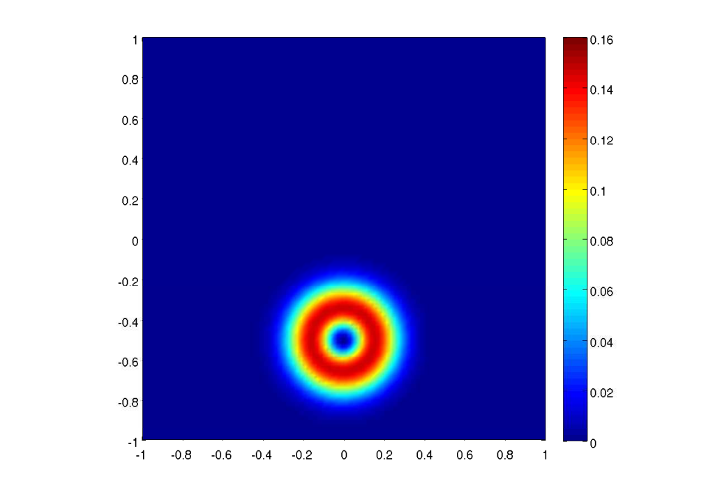
As shown in this figure, $SBP2$ and $SBP4$ schemes resolve the solution quite well. In fact, $SBP4$ is very accurate and keeps the hump intact throughout the rotation.

In Table 4.1, we present percentage relative errors in $l^{2}$. The errors are computed at time $t=2\pi$ (one rotation) on a sequence of meshes for both the $SBP2$ and $SBP4$ schemes. The results show that the errors are quite low, particularly for $SBP4$ and the rate of convergence approaches the expected values of $2$ for $SBP2$ and $3$ for $SBP4$. Furthermore, the order of accuracy is unaffected at these resolutions by using zero Dirichlet boundary data instead of the exact solution at the boundary.

We have considered a fully-discrete scheme for the magnetic induction equations that arise as a submodel in the MHD equations of plasma physics. In future, our plan is to extend the semi-discrete scheme given in [6] to a semi-implicit fully-discrete scheme. We would like to show the stabilty of the aforementioned semi-implicit scheme in case of magnetic induction equations with resistivity.

References

- [1] N. Besse and D. Kröner. Convergence of the locally divergence free discontinuous Galerkin methods for induction equations for the 2D-MHD system. M2AN Math. Model. Num. Anal 39(6):1177-1202, 2005.
- [2] J.U. Brackbill and D.C. Barnes. The effect of nonzero on the numerical solution of the magnetohydrodynamic equations. J. Comp. Phys., 35:426-430, 1980.
- [3] W. Dai and P.R. Woodward. A simple finite difference scheme for multi-dimensional magnetohydrodynamic equations. J. Comp. Phys., 142(2):331-369, 1998.
- [4] F. Fuchs, K.H. Karlsen, S. Mishra and N.H. Risebro. Stable upwind schemes for the Magnetic Induction equation. Preprint, Submitted.
- [5] U. Koley, S. Mishra, N.H. Risebro and M. Svärd. Higher order finite difference schemes for the Magnetic Induction equations. BIT Numer Math., 49: 375-395 (2009).
- [6] U. Koley, S. Mishra, N.H. Risebro and M. Svärd. Higher order finite difference schemes for the Magnetic Induction equations with resistivity. Preprint, Submitted.
- [7] B. Gustafsson, H.-O. Kreiss, and J. Oliger. Time dependent problems and difference methods. John Wiley & Sons, Inc., 1995.
- [8] S. Mishra and M. Svärd. On stability of numerical schemes via frozen coefficients and magnetic induction equations. Preprint, Submitted.
- [9] M. Svärd On coordinate transformations for summation-by-parts operators J. Sci. Comput. 20(2004), 29-42.
- [10] M. Svärd and J. Nordström. On the order of accuracy for difference approximations of initial-boundary value problems. Journal of Computational Physics, 218(2006), 333-352.
- [11] M. Torrilhon and M. Fey. Constraint-preserving upwind methods for multidimensional advection equations. SIAM. J. Num. Anal., 42(4):1694-1728, 2004.