跳到论文正文
W Papers独立论文阅读器 arXiv:1102.0493 论文正文 计算阅读时间 · 0%
引用这篇论文根据当前论文元数据生成,正式投稿前建议核对。


License: arXiv.org perpetual non-exclusive license
arXiv:1102.0493v2 [math.AP] 18 Sep 2012

An error estimate for the finite difference approximation to degenerate convection - diffusion equations

K. H. Karlsen Kenneth Hvistendahl Karlsen
Centre of Mathematics for Applications (CMA)
University of Oslo
P.O. Box 1053, Blindern
N–0316 Oslo, Norway
Email address: kennethk@math.uio.no
, U. Koley Ujjwal Koley
Centre of Mathematics for Applications (CMA)
University of Oslo
P.O. Box 1053, Blindern
N–0316 Oslo, Norway
Email address: ujjwalk@cma.uio.no
and N. H. Risebro Nils Henrik Risebro
Centre of Mathematics for Applications (CMA)
University of Oslo
P.O. Box 1053, Blindern
N–0316 Oslo, Norway
Email address: nilshr@math.uio.no
Date: August 24, 2026
Abstract.

We consider semi-discrete first-order finite difference schemes for a nonlinear degenerate convection-diffusion equations in one space dimension, and prove an L1L^{1} error estimate. Precisely, we show that the Lloc1L^{1}_{\mathrm{loc}} difference between the approximate solution and the unique entropy solution converges at a rate 𝒪⁡(Δ​x1/11)\mathcal{O}(\Delta x^{1/11}), where Δ​x\Delta x is the spatial mesh size. If the diffusion is linear, we get the convergence rate 𝒪⁡(Δ​x1/2)\mathcal{O}(\Delta x^{1/2}), the point being that the 𝒪\mathcal{O} is independent of the size of the diffusion.

Key words and phrases: 
degenerate convection-diffusion equations, entropy conditions, finite difference schemes, rate of convergence

1. Introduction

In this paper, we consider semi-discrete finite difference schemes for the following Cauchy problem

(1.1) {ut+f​(u)x=A​(u)x​x,(x,t)∈ΠT,u⁡(0,x)=u0​(x),x∈ℝ,\begin{cases}u_{t}+f(u)_{x}=A(u)_{xx},&(x,t)\in\Pi_{T},\\ u(0,x)=u_{0}(x),&x\in\mathbb{R},\end{cases}

where ΠT=ℝ×(0,T)\Pi_{T}=\mathbb{R}\times(0,T) with T>0T>0 fixed, u:ΠT→ℝu:\Pi_{T}\to\mathbb{R} is the unknown function, ff the flux function, and AA the nonlinear diffusion. Regarding this, the basic assumption is that A′≥0A^{\prime}\geq 0, and thus (1.1) is a strongly degenerate parabolic problem. The scalar conservation law ut+f​(u)x=0u_{t}+f(u)_{x}=0 is a special example of this type of problems. Other examples occur in several applications, for instance in porous media flow [9] and in sedimentation processes [3].

Since A′A^{\prime} may be zero, solutions are not necessary smooth and one must consider weak solutions. These are not necessarily uniquely determined by the initial data, and in order to get uniqueness, one considers so-called entropy solutions. The framework of entropy solutions makes the initial value problem (1.1) well posed, for a precise statement, see Section 2. For scalar conservation laws, the entropy framework (usually called entropy conditions) was introduced by Kružkov [24] and Vol’pert [30], while for degenerate parabolic equations entropy solution were first considered by Vol’pert and Hudajev [31]. Uniqueness of entropy solutions to (1.1) was first proved by Carrillo [4], see also Karlsen and Risebro [20].

For hyperbolic equations, the convergence analysis of difference schemes has a long tradition, we mention only a few references. Finite difference schemes have been studied by Oleĭnik [28], Harten et al. [17], Kuznetsov [26], Crandall and Majda [8], Osher and Tadmor [29], Cockburn and Gripenberg. [6], Kröner and Rokyta [23], Eymard et al. [14], Noelle [32] as well as many others.

In the last decade, there has been a growing interest in numerical approximation of entropy solutions to degenerate parabolic equations. Finite difference and finite volume schemes for degenerate equations were analysed by Evje and Karlsen [10, 11, 12, 13] (using upwind difference schemes), Holden et al. [18, 19] (using operator splitting methods), Kurganov and Tadmor [25] (central difference schemes), Bouchut et al. [2] (kinetic BGK schemes), Afif and Amaziane [1] and Ohlberger, Gallouët et al. [27, 16, 15] (finite volume methods), Cockburn and Shu [7] (discontinuous Galerkin methods) and Karlsen and Risebro [22, 21] (monotone difference schemes). Many of the above papers show that the approximate solutions converge to the unique entropy solution as the discretization parameter vanishes.

Despite this relatively large body of research, to the best of our knowledge, there does not exist a result giving the convergence rate of the approximate solutions to degenerate problems. For conservation laws (very degenerate problems), the convergence rate for monotone methods has long been known to be Δ​x1/2\Delta x^{1/2} [26], and this is also optimal for discontinuous solutions. For non-degenerate problems, the solution operator (taking initial data to the corresponding solution) has a strong smoothing effect, and truncation analysis applies. Hence difference methods produces approximations converging at the formal order of the scheme. However, all estimates depend on A′A^{\prime}, and are not available if A′A^{\prime} is not bounded below by some positive number η\eta.

Often, the viscous regualarization

(1.2) utη+f​(uη)x=A​(uη)x​x+η​ux​xη,u^{\eta}_{t}+f(u^{\eta})_{x}=A(u^{\eta})_{xx}+\eta u^{\eta}_{xx},

is used to model the behaviour of first order difference schemes. The rationale behind this is that first order schemes for (1.1) are formally second order accurate for an equation resembling (1.2). If one can prove convergence, or find a convergence rate, such that uη→uu^{\eta}\to u, then often analogous arguments will work for appropriate difference schemes. If this convergence has a rate, it is expected that the difference scheme will have the same rate. In [13], Evje and Karlsen showed that

‖uη​(⋅,t)−u⁡(⋅,t)‖L1​(ℝ)=𝒪⁡(η1/2).\left\|u^{\eta}(\cdot,t)-u(\cdot,t)\right\|_{L^{1}(\mathbb{R})}=\mathcal{O}\left(\eta^{1/2}\right).

Also, in [15], Gallouët et al. showed for the boundary value problem corresponding to (1.1) that

‖uη​(⋅,t)−u⁡(⋅,t)‖L1​(ℝ)=𝒪⁡(η1/5).\left\|u^{\eta}(\cdot,t)-u(\cdot,t)\right\|_{L^{1}(\mathbb{R})}=\mathcal{O}\left(\eta^{1/5}\right).

To show the same rate for a difference scheme seems remarkably difficult. The main result of this paper is that we prove a significantly lower convergence rate for a semi-discrete difference approximation uΔ​xu_{\Delta x},

∫−L+M​tL−M​t|u⁡(x,t)−uΔ​x​(x,t)|​𝑑x≤𝒪⁡(Δ​x1/11),\int_{-L+Mt}^{L-Mt}\left|u(x,t)-u_{\Delta x}(x,t)\right|\,dx\leq\mathcal{O}\left(\Delta x^{1/11}\right),

where MM is a constant larger than |f′|\left|f^{\prime}\right|. The 𝒪\mathcal{O} symbol depends on tt, LL and the initial data u0u_{0}, but not on the discretization parameter Δ​x\Delta x.

The rest of this paper is organized as follows. In Section 2 we make precise the definition of a solution of (1.1), and of uΔ​xu_{\Delta x}. Then we list a number of useful properties of the (unique) weak solution and of the approximation uΔ​xu_{\Delta x}. Finally we state our main theorem. Section 3 is devoted to its proof, while we test the practical convergence properties of the scheme on a numerical example in Section 4.

2. Preliminaries

Independently of the smoothness of the initial data, due to the degeneracy of the diffusion, jumps may form in the solution uu. Therefore we consider solutions in the weak sense, i.e.,

Definition 2.1.

Set ΠT=(0,T)×ℝ\Pi_{T}=(0,T)\times\mathbb{R}, a function u⁡(t,x)∈L∞​((0,T),L1​(ℝ))∩L∞​(ΠT)u(t,x)\in L^{\infty}\left((0,T);L^{1}(\mathbb{R})\right)\cap L^{\infty}(\Pi_{T}) is a weak solution of the initial value problem (1.1) if it satisfies

  1. D.1

    A⁡(u)A(u) is continuous and A​(u)x∈L∞​(ΠT)A(u)_{x}\in L^{\infty}(\Pi_{T}).

  2. D.2

    For all test functions φ∈𝒟⁡(ΠT)\varphi\in\mathcal{D}(\Pi_{T})

    (2.1) ∬ΠTu​φt+f⁡(u)​φx+A⁡(u)​φx​x​𝑑x​𝑑t=0.\iint_{\Pi_{T}}u\varphi_{t}+f(u)\varphi_{x}+A(u)\varphi_{xx}\,dxdt=0.
  3. D.3

    The initial condition is satisfied in the L1L^{1}-sense

    limt↓0∫ℝ|u⁡(t,x)−u0​(x)|​𝑑x=0.\lim_{t\downarrow 0}\int_{\mathbb{R}}\left|u(t,x)-u_{0}(x)\right|\,dx=0.

In view of the existence theory, the condition D.1 is natural, and thanks to this we can replace (2.1) by

(2.2) ∬ΠTu​φt+(f⁡(u)−A​(u)x)​φx​𝑑x​𝑑t=0.\iint_{\Pi_{T}}u\varphi_{t}+\left(f(u)-A(u)_{x}\right)\varphi_{x}\,dxdt=0.

If AA is constant on a whole interval, then weak solutions are not uniquely determined by their initial data, and one must impose an additional entropy condition to single out the physically relevant solution. A weak solution satisfies the entropy condition if

(2.3) ϱ​(u)t+q​(u)x+r​(u)x​x≤0​in 𝒟′​(ΠT),\varrho(u)_{t}+q(u)_{x}+r(u)_{xx}\leq 0\ \text{in $\mathcal{D}^{\prime}(\Pi_{T})$,}

for all convex, twice differentiable functions ϱ:ℝ→ℝ\varrho:\mathbb{R}\to\mathbb{R}, where qq and rr are defined by

q′​(u)=ϱ′​(u)​f′​(u),and​r′​(u)=ϱ′​(u)​A′​(u).q^{\prime}(u)=\varrho^{\prime}(u)f^{\prime}(u),\ \text{and}\ r^{\prime}(u)=\varrho^{\prime}(u)A^{\prime}(u).

Via a standard limiting argument this implies that (2.3) holds for the Kružkov entropies ϱ⁡(u)=|u−c|\varrho(u)=\left|u-c\right| for all constants cc. We say that a weak solution satisfying the entropy condition is an entropy solution.

Let the signum function be defined as

sign⁡(σ)={−1σ<0,0σ=0,1σ>0,\mathrm{sign}(\sigma)=\begin{cases}-1&\sigma<0,\\ 0&\sigma=0,\\ 1&\sigma>0,\end{cases}

and its regularized counterpart, signε\mathrm{sign}_{\varepsilon}, defined as

signε​(σ)={sign⁡(σ)|σ|>ε,sin⁡(π​σ2​ε)otherwise,\mathrm{sign}_{\varepsilon}(\sigma)=\begin{cases}\mathrm{sign}(\sigma)&\left|\sigma\right|>\varepsilon,\\ \sin\left(\frac{\pi\sigma}{2\varepsilon}\right)&\text{otherwise,}\end{cases}

where ε>0\varepsilon>0.

We collect some useful information about entropy solutions in the following, for a proof see [13].

Theorem 2.1.

The unique entropy solution uu of (1.1) satisfies

(2.4) ∬ΠT|u−c|​φt+sign⁡(u−c)​(f⁡(u)−f⁡(c))​φx+|A⁡(u)−A⁡(c)|​φx​x​𝑑x​𝑑t≥0,\iint_{\Pi_{T}}\left|u-c\right|\varphi_{t}+\mathrm{sign}(u-c)(f(u)-f(c))\varphi_{x}+\left|A(u)-A(c)\right|\varphi_{xx}\,dxdt\geq 0,

for all constants cc and all non-negative test functions in 𝒟′​(ΠT)\mathcal{D}^{\prime}(\Pi_{T}). Furthermore, the following limits hold, provided AA is strictly increasing,

(2.5) ∬ΠT|u−c|​φt+\displaystyle\iint_{\Pi_{T}}\left|u-c\right|\varphi_{t}+ sign⁡(u−c)​(f⁡(u)−f⁡(c)−A​(u)x)​φx\displaystyle\mathrm{sign}(u-c)\left(f(u)-f(c)-A(u)_{x}\right)\varphi_{x}
=limε↓0∬ΠT|A​(u)x|2​signε′​(A⁡(u)−A⁡(c))​φ​dt​dx,\displaystyle=\lim_{\varepsilon\downarrow 0}\iint_{\Pi_{T}}\left|A(u)_{x}\right|^{2}\mathrm{sign}^{\prime}_{\varepsilon}\left(A(u)-A(c)\right)\,\varphi\,dtdx,
(2.6) limε↓0∬ΠT(f⁡(u)−f⁡(c))​A​(u)x​signε′​(A⁡(u)−A⁡(c))​φ​𝑑t​𝑑x=0,\lim_{\varepsilon\downarrow 0}\iint_{\Pi_{T}}\left(f(u)-f(c)\right)A(u)_{x}\,\mathrm{sign}^{\prime}_{\varepsilon}\left(A(u)-A(c)\right)\varphi\,dtdx=0,

for all non-negative test functions φ\varphi.

A common method to show existence of an entropy solution is to consider the regularized problem

(2.7) utη+f​(uη)x=(A⁡(uη)+η​u)x​x,t>0,uη​(0,x)=u0​(x),u^{\eta}_{t}+f\left(u^{\eta}\right)_{x}=\left(A\left(u^{\eta}\right)+\eta u\right)_{xx},\ t>0,\quad u^{\eta}(0,x)=u_{0}(x),

where η\eta is some (small) positive number. This equation is not degenerate, and has a unique smooth solution for t>0t>0. The sequence {uη}η>0\left\{u^{\eta}\right\}_{\eta>0} is compact in L1​(ΠT)L^{1}(\Pi_{T}), and converges to the entropy solution. In [13], it was established that for t<Tt<T

(2.8) ‖u⁡(t,⋅)−uη​(t,⋅)‖L1​(ℝ)≤C​η,\left\|u(t,\cdot)-u^{\eta}(t,\cdot)\right\|_{L^{1}(\mathbb{R})}\leq C\sqrt{\eta},

where the constant CC only depends on ff, AA and the initial data u0u_{0}. Of course, uηu^{\eta} is also an entropy solution to (2.7), where the diffusion function is given by

Aη​(u)=A⁡(u)+η​u.A^{\eta}(u)=A(u)+\eta u.

Rather than discretizing (1.1), we shall discretize the regularized equation (2.7), and let η\eta tend to zero in a suitable manner. Due to (2.8), it suffices to compare uηu^{\eta} and our approximate solution. To simplify our notation, we therefore, for the moment, assume that AA is strictly increasing, with A′​(u)≥η>0A^{\prime}(u)\geq\eta>0.

We consider a semi-discrete approximation, where space is discrete, but time continuous. Let Δ​x\Delta x be some small parameter, and set xj=j​Δ​xx_{j}=j\Delta x and xj+1/2=(j+1/2)​Δ​xx_{j+1/2}=(j+1/2)\Delta x for j∈ℤj\in{\mathbb{Z}}. Set Ij=(xj−1/2,xj+1/2]I_{j}=(x_{j-1/2},x_{j+1/2}]. The discrete derivatives D±D^{\pm} are defined by

D±​σj=±σj±1−σjΔ​x.D^{\pm}\sigma_{j}=\pm\frac{\sigma_{j\pm 1}-\sigma_{j}}{\Delta x}.

Our scheme is defined by

(2.9) {dd​t​uj​(t)+D−​Fj+1/2=D−​D+​Aj,t>0,uj​(0)=1Δ​x​∫Iju0​(x)​dx,\begin{cases}\frac{d}{dt}u_{j}(t)+D^{-}F_{j+1/2}=D^{-}D^{+}A_{j},&t>0,\\ u_{j}(0)=\frac{1}{\Delta x}\int_{I_{j}}u_{0}(x)\,dx,\end{cases}

for j∈ℤj\in{\mathbb{Z}}. Here Fi+1/2F_{i+1/2} is the Engquist-Osher flux and Aj=A⁡(uj)A_{j}=A\left(u_{j}\right). More precisely, for a monotone flux ff, the generalized upwind scheme of Engquist and Osher is defined by

Fj+12=F⁡(uj,uj+1)=f+​(uj)+f−​(uj+1),\displaystyle F_{j+\frac{1}{2}}=F(u_{j},u_{j+1})=f^{+}(u_{j})+f^{-}(u_{j+1}),

where

f+​(u)=f⁡(0)+∫0umax⁡(f′​(s),0)​𝑑s,f−​(u)=∫0umin⁡(f′​(s),0)​𝑑s.\displaystyle f^{+}(u)=f(0)+\int_{0}^{u}\max\left(f^{\prime}(s),0\right)\,ds,\qquad f^{-}(u)=\int_{0}^{u}\min\left(f^{\prime}(s),0\right)\,ds.

With this, we can rewrite our scheme (2.9) as

(2.10) {dd​t​uj​(t)+(D−​f+​(uj)+D+​f−​(uj))=D−​D+​Aj,t>0,uj​(0)=1Δ​x​∫Iju0​(x)​dx,\begin{cases}\frac{d}{dt}u_{j}(t)+\left(D^{-}f^{+}(u_{j})+D^{+}f^{-}(u_{j})\right)=D^{-}D^{+}A_{j},&t>0,\\ u_{j}(0)=\frac{1}{\Delta x}\int_{I_{j}}u_{0}(x)\,dx,\end{cases}

for j∈ℤj\in{\mathbb{Z}} and Aj=A⁡(uj)A_{j}=A\left(u_{j}\right).

In order to define an approximation on the whole of ΠT\Pi_{T}, we let uΔ​xu_{\Delta x} be the piecewise linear interpolant given by

uΔ​x(x,t)=uj(t)+D+uj(t)(x−xj),for x∈[xj,xj+1],u_{\Delta x}(x,t)=u_{j}(t)+D^{+}u_{j}(t)\left(x-x_{j}\right),\quad\text{for $x\in[x_{j},x_{j+1}]$,}

and with a slight abuse of notation we define uju_{j} to be the piecewise constant (in xx) function

uj​(x,t)=uj​(t)for x∈(xj−1/2,xj+1/2].u_{j}(x,t)=u_{j}(t)\quad\text{for $x\in(x_{j-1/2},x_{j+1/2}]$.}

We collect some useful results regarding uΔ​xu_{\Delta x} and the entropy solution uu in the next lemma.

Lemma 2.1.

If uu is the unique entropy solution of (1.1) and uju_{j} the function defined by the scheme (2.9). Then the following estimates hold:

(2.11) ‖u⁡(⋅,t)‖L∞​(ℝ)\displaystyle\left\|u(\cdot,t)\right\|_{L^{\infty}(\mathbb{R})} ≤‖u0‖L∞​(ℝ)\displaystyle\leq\left\|u_{0}\right\|_{L^{\infty}(\mathbb{R})}
(2.12) |u⁡(⋅,t)|B.V.(ℝ)\displaystyle\left|u(\cdot,t)\right|_{B.V.(\mathbb{R})} ≤|u0|B.V.(ℝ)\displaystyle\leq\left|u_{0}\right|_{B.V.(\mathbb{R})}
(2.13) ‖f⁡(u⁡(⋅,t))−A​(u⁡(⋅,t))x‖L∞​(ℝ)\displaystyle\left\|f(u(\cdot,t))-A(u(\cdot,t))_{x}\right\|_{L^{\infty}(\mathbb{R})} ≤‖f⁡(u0)−A​(u0)x‖L∞​(ℝ)\displaystyle\leq\left\|f(u_{0})-A(u_{0})_{x}\right\|_{L^{\infty}(\mathbb{R})}
(2.14) |f⁡(u⁡(⋅,t))−A​(u⁡(⋅,t))x|B.V.(ℝ)\displaystyle\left|f(u(\cdot,t))-A(u(\cdot,t))_{x}\right|_{B.V.(\mathbb{R})} ≤|f⁡(u0)−A​(u0)x|B.V.(ℝ)\displaystyle\leq\left|f(u_{0})-A(u_{0})_{x}\right|_{B.V.(\mathbb{R})}
(2.15) ‖uj​(t)‖L∞​(ℝ)\displaystyle\left\|u_{j}(t)\right\|_{L^{\infty}(\mathbb{R})} ≤‖uj​(0)‖L∞​(ℝ)\displaystyle\leq\left\|u_{j}(0)\right\|_{L^{\infty}(\mathbb{R})}
(2.16) |uj​(t)|B.V.(ℝ)\displaystyle\left|u_{j}(t)\right|_{B.V.(\mathbb{R})} ≤|uj​(0)|B.V.(ℝ)\displaystyle\leq\left|u_{j}(0)\right|_{B.V.(\mathbb{R})}
(2.17) ‖Fj+1/2​(t)−D+​A​(uj​(t))‖L∞​(ℝ)\displaystyle\left\|F_{j+1/2}(t)-D^{+}A\left(u_{j}(t)\right)\right\|_{L^{\infty}(\mathbb{R})} ≤‖Fj+1/2​(0)−D+​A​(uj​(0))‖L∞​(ℝ)\displaystyle\leq\left\|F_{j+1/2}(0)-D^{+}A\left(u_{j}(0)\right)\right\|_{L^{\infty}(\mathbb{R})}
(2.18) |Fj+1/2​(t)−D+​A​(uj​(t))|B.V.(ℝ)\displaystyle\left|F_{j+1/2}(t)-D^{+}A\left(u_{j}(t)\right)\right|_{B.V.(\mathbb{R})} ≤|Fj+1/2​(0)−D+​A​(uj​(0))|B.V.(ℝ).\displaystyle\leq\left|F_{j+1/2}(0)-D^{+}A\left(u_{j}(0)\right)\right|_{B.V.(\mathbb{R})}.

In addition the initial error is bounded by

(2.19) ‖uΔ​x​(⋅,0)−u0‖L1​(ℝ)≤C​Δ​x,\left\|u_{\Delta x}(\cdot,0)-u_{0}\right\|_{L^{1}(\mathbb{R})}\leq C\Delta x,

for some constant CC which depends only on |u0|B.V.(ℝ)\left|u_{0}\right|_{B.V.(\mathbb{R})}.

For a proof of this, see [13]. Note that if u0u_{0} and A​(u0)xA(u_{0})_{x} (and uj​(0)u_{j}(0) and D+​A​(uj​(0))D^{+}A(u_{j}(0))) are bounded independently of η\eta (and Δ​x\Delta x), then (2.13) and (2.17) imply that

(2.20) ‖D+​A​(uj)‖L∞​(ℝ)≤C​and​‖A​(u)x‖L∞​(ℝ)≤C,\left\|D^{+}A(u_{j})\right\|_{L^{\infty}(\mathbb{R})}\leq C\ \text{and}\ \left\|A(u)_{x}\right\|_{L^{\infty}(\mathbb{R})}\leq C,

for some constant CC which is independent of Δ​x\Delta x and η\eta.

Our main result is the following

Main Theorem.

Let uu be the unique entropy solution to (1.1) and uΔ​xu_{\Delta x} be as defined by (2.10). Choose a constant

M>max|u|<‖u0‖L∞​(ℝ)⁡|f′​(u)|,M>\max_{\left|u\right|<\left\|u_{0}\right\|_{L^{\infty}(\mathbb{R})}}\left|f^{\prime}(u)\right|,

and another constant L>M​TL>MT, where T>0T>0. Then there exists a constant CC, independent of Δ​x\Delta x, but depending on ff, LL, TT and u0u_{0}, such that

∫L+M​tL−M​t|u⁡(t,x)−uΔ​x​(t,x)|​𝑑x≤C​Δ​x1/11for t≤T.\int_{L+Mt}^{L-Mt}\left|u(t,x)-u_{\Delta x}(t,x)\right|\,dx\leq C\Delta x^{1/11}\quad\text{for $t\leq T$.}

As a by-product of our method of proof we get an improved rate if the diffusion is linear. The significance of this rate is that is independent of the size of the diffusion, which in this case is η\eta.

Main Corollary.

Let uu be the unique solution to the viscous regularization

ut+f​(u)x=η​ux​x,t>0,u⁡(x,0)=u0​(x),u_{t}+f(u)_{x}=\eta u_{xx},\ t>0,\quad u(x,0)=u_{0}(x),

and let uΔ​xu_{\Delta x} be defined by (2.10) with A⁡(u)=η​uA(u)=\eta u. Then there exists a constant CC, independent of Δ​x\Delta x and η\eta, but depending on ff, LL, TT and u0u_{0}, such that

∫L+M​tL−M​t|u⁡(t,x)−uΔ​x​(t,x)|​𝑑x≤C​Δ​x1/2for t≤T.\int_{L+Mt}^{L-Mt}\left|u(t,x)-u_{\Delta x}(t,x)\right|\,dx\leq C\Delta x^{1/2}\quad\text{for $t\leq T$.}

In the linear case this is what we expect. In fact, in [5] Chen and Karlsen showed that for a linear flux function ff the expected η\eta independent rate of 1/21/2 holds. However, the methods used in [5] are not easily modified to nonlinear flux functions.

3. Proof of the main theorem

First of all, for simplicity we will prove the main theorem for f′<0f^{\prime}<0. Note that, in that case Fj+1/2=f⁡(uj+1)F_{j+1/2}=f(u_{j+1}). The general case treatment will be similar (see Remark  3.1). The theorem will be proved by a “doubling of the variables” argument, but we start not with the entropy condition (2.5), but in the argument leading up to this condition. Set

ψε​(u,c)=∫cusignε​(A⁡(z)−A⁡(c))​𝑑z.\psi_{\varepsilon}(u,c)=\int_{c}^{u}\mathrm{sign}_{\varepsilon}\left(A(z)-A(c)\right)\,dz.

This is a convex entropy for all constants cc. Set u=u⁡(y,s)u=u(y,s) and rewrite (1.1) as

us+(f⁡(u)−f⁡(c))y=(A⁡(u)−A⁡(c))y​y,u_{s}+\left(f(u)-f(c)\right)_{y}=\left(A(u)-A(c)\right)_{yy},

and multiply this with ψε′​(u,c)​φ\psi^{\prime}_{\varepsilon}(u,c)\varphi where φ\varphi is a test function with compact support in ℝ×(0,T)\mathbb{R}\times(0,T). Remember that A′≥η>0A^{\prime}\geq\eta>0, so uu is smooth, after a partial integration, we arrive at

∬ΠTψε​(u,c)​φs+Qϵ​(u,c)​φy​𝑑y​𝑑s\displaystyle\iint_{\Pi_{T}}\psi_{\varepsilon}(u,c)\varphi_{s}+Q_{\epsilon}(u,c)\varphi_{y}\,dyds
=∬ΠTsignε​(A⁡(u)−A⁡(c))​A​(u)y​φy+signε′​(A⁡(u)−A⁡(c))​(A​(u)y)2​φ​𝑑y​𝑑s.\displaystyle\qquad=\iint_{\Pi_{T}}\mathrm{sign}_{\varepsilon}\left(A(u)-A(c)\right)A(u)_{y}\varphi_{y}+\mathrm{sign}_{\varepsilon}^{\prime}\left(A(u)-A(c)\right)\left(A(u)_{y}\right)^{2}\varphi\,dyds.

Where we have used Qε′​(u,c)=ψε′​(u,c)​f′​(u)Q^{\prime}_{\varepsilon}(u,c)=\psi^{\prime}_{\varepsilon}(u,c)f^{\prime}(u). Although ψε​(u,c)≈|u−c|\psi_{\varepsilon}(u,c)\approx\left|u-c\right|, ψε\psi_{\varepsilon} is not symmetric in uu and cc. This makes it cumbersome to work with when doubling the variables, so we rewrite the above as

(3.1) ∬ΠT\displaystyle\iint_{\Pi_{T}} |u−c|​φs+Qϵ​(u,c)​φy​d​y​d​s\displaystyle\left|u-c\right|\varphi_{s}+Q_{\epsilon}(u,c)\varphi_{y}\,dyds
=∬ΠTsignε′​(A⁡(u)−A⁡(c))​(A​(u)y)2​φ+signε​(A⁡(u)−A⁡(c))​A​(u)y​φy\displaystyle=\iint_{\Pi_{T}}\mathrm{sign}_{\varepsilon}^{\prime}\left(A(u)-A(c)\right)\left(A(u)_{y}\right)^{2}\varphi+\mathrm{sign}_{\varepsilon}\left(A(u)-A(c)\right)A(u)_{y}\varphi_{y}
+(|u−c|−ψε​(u,c))​φs​d​y​d​s.\displaystyle+\left(\left|u-c\right|-\psi_{\varepsilon}(u,c)\right)\varphi_{s}\,dyds.

In the doubling of variables argument we choose c=uΔ​x​(x,t)c=u_{\Delta x}(x,t), and a test function φ⁡(x,y,t,s)\varphi(x,y,t,s). Integrating the above over (x,t)∈ΠT(x,t)\in\Pi_{T} after an integration by parts, we end up with

(3.2) ∫ΠT2|u−uΔ​x|​φs+signε​(A⁡(u)−A⁡(uΔ​x))​(f⁡(u)−f⁡(uΔ​x))​φy​𝑑X=∫ΠT2[sign′ε(A(u)−A(uΔ​x))((A(u)y)2−A(u)yA(uΔ​x)x)φ−|A⁡(u)−A⁡(uΔ​x)|ε​(φy​y+φx​y)+(ψε​(u,uΔ​x)−|u−uΔ​x|)​φs+(∫uΔ​xudd​z(signε(A(z)−A(uΔ​x)))(f(z)−f(uΔ​x))dz)φy]dX,\int_{\Pi_{T}^{2}}\left|u-u_{\Delta x}\right|\varphi_{s}+\mathrm{sign}_{\varepsilon}(A(u)-A(u_{\Delta x}))(f(u)-f(u_{\Delta x}))\varphi_{y}\,dX\\ =\int_{\Pi_{T}^{2}}\Bigl[\mathrm{sign}^{\prime}_{\varepsilon}\left(A(u)-A\left(u_{\Delta x}\right)\right)\left(\left(A(u)_{y}\right)^{2}-A(u)_{y}A\left(u_{\Delta x}\right)_{x}\right)\varphi\\ -\left|A(u)-A\left(u_{\Delta x}\right)\right|_{\varepsilon}\left(\varphi_{yy}+\varphi_{xy}\right)+\left(\psi_{\varepsilon}\left(u,u_{\Delta x}\right)-\left|u-u_{\Delta x}\right|\right)\varphi_{s}\\ +\left(\int_{u_{\Delta x}}^{u}\frac{d}{dz}(\mathrm{sign}_{\varepsilon}(A(z)-A(u_{\Delta x})))(f(z)-f(u_{\Delta x}))\,dz\right)\varphi_{y}\Bigr]\,dX,

where d​X=d​y​d​s​d​x​d​tdX=dydsdxdt and |a|ε=∫0asignε​(z)​𝑑z\left|a\right|_{\varepsilon}=\int^{a}_{0}\mathrm{sign}_{\varepsilon}(z)dz. Here we have used that

0\displaystyle 0 =∫ΠT2(signε​(A⁡(u)−A⁡(uΔ​x))​A​(u)y​φ)x​𝑑X\displaystyle=\int_{\Pi_{T}^{2}}\left(\mathrm{sign}_{\varepsilon}\left(A(u)-A(u_{\Delta x})\right)A(u)_{y}\varphi\right)_{x}\,dX
=∫ΠT2signε′​(A⁡(u)−A⁡(uΔ​x))​A​(u)y​A​(uΔ​x)x​φ−|A⁡(u)−A⁡(uΔ​x)|ε​φx​y​𝑑X,\displaystyle=\int_{\Pi_{T}^{2}}\mathrm{sign}_{\varepsilon}^{\prime}\left(A(u)-A(u_{\Delta x})\right)A(u)_{y}A(u_{\Delta x})_{x}\varphi-\left|A(u)-A\left(u_{\Delta x}\right)\right|_{\varepsilon}\varphi_{xy}\,dX,

and that

∫ΠT2signε​(A⁡(u)−A⁡(uΔ​x))​A​(u)y​φy​𝑑X\displaystyle\int_{\Pi_{T}^{2}}\mathrm{sign}_{\varepsilon}\left(A(u)-A(u_{\Delta x})\right)A(u)_{y}\varphi_{y}\,dX =∫ΠT2(|A⁡(u)−A⁡(uΔ​x)|ε)y​φy​𝑑X\displaystyle=\int_{\Pi_{T}^{2}}\left(\left|A(u)-A\left(u_{\Delta x}\right)\right|_{\varepsilon}\right)_{y}\varphi_{y}\,dX
=−∫ΠT2|A(u)−A(uΔ​x)|εφy​ydX.\displaystyle=-\int_{\Pi_{T}^{2}}\left|A(u)-A\left(u_{\Delta x}\right)\right|_{\varepsilon}\varphi_{yy}\,dX.

Also

Qε​(u,uΔ​x)\displaystyle Q_{\varepsilon}(u,u_{\Delta x}) =∫uΔ​xusignε​(A⁡(z)−A⁡(uΔ​x))​dd​z​(f⁡(z)−f⁡(uΔ​x))​𝑑z\displaystyle=\int_{u_{\Delta x}}^{u}\mathrm{sign}_{\varepsilon}(A(z)-A(u_{\Delta x}))\frac{d}{dz}(f(z)-f(u_{\Delta x}))\,dz
=−∫uΔ​xudd​z(signε(A(z)−A(uΔ​x)))(f(z)−f(uΔ​x))dz\displaystyle=-\int_{u_{\Delta x}}^{u}\frac{d}{dz}(\mathrm{sign}_{\varepsilon}(A(z)-A(u_{\Delta x})))(f(z)-f(u_{\Delta x}))\,dz
+signε​(A⁡(u)−A⁡(uΔ​x))​(f⁡(u)−f⁡(uΔ​x)).\displaystyle\qquad\qquad+\mathrm{sign}_{\varepsilon}(A(u)-A(u_{\Delta x}))(f(u)-f(u_{\Delta x})).

The next goal is to obtain an analogous estimate for the difference approximation uΔ​xu_{\Delta x}. Set φj​(t)=φ⁡(xj,t)\varphi_{j}(t)=\varphi(x_{j},t) and multiply the scheme (2.9) with ψε′​(uj,c)​φj\psi_{\varepsilon}^{\prime}(u_{j},c)\varphi_{j} and do a summation by parts to get

∑j[ψ​(uj,c)t​φj+φj​D+​Qϵ​(uj,c)]\displaystyle\sum_{j}\Bigl[\psi\left(u_{j},c\right)_{t}\varphi_{j}+\varphi_{j}D^{+}Q_{\epsilon}(u_{j},c)\Bigr]
=−∑jψε′(uj,c)D+A(uj)D+φj+D+ψε′(uj,c)D+A(uj)φj+1\displaystyle=-\sum_{j}\psi_{\varepsilon}^{\prime}\left(u_{j},c\right)D^{+}A\left(u_{j}\right)D^{+}\varphi_{j}+D^{+}\psi_{\varepsilon}^{\prime}\left(u_{j},c\right)D^{+}A\left(u_{j}\right)\varphi_{j+1}
+∑jφjΔ​x∫ujuj+1ψε(s,c)′′(f(uj+1)−f(s))ds.\displaystyle\qquad\qquad+\sum_{j}\frac{\varphi_{j}}{\Delta x}\int_{u_{j}}^{u_{j+1}}\psi_{\varepsilon}{{}^{\prime\prime}}\left(s,c\right)(f(u_{j+1})-f(s))\,ds.

Where we have used the following result:

0≥∫ujuj+1ψε′′(s,c)[f(uj+1)−f(s)]ds=∫ujuj+1ψε′(s,c)\displaystyle 0\geq\int_{u_{j}}^{u_{j+1}}\psi_{\varepsilon}^{{}^{\prime\prime}}(s,c)[f(u_{j+1})-f(s)]\,ds=\int_{u_{j}}^{u_{j+1}}\psi_{\varepsilon}^{{}^{\prime}}(s,c) f′​(s)​d​s\displaystyle f^{\prime}(s)\,ds
−ψε′​(uj)​[f⁡(uj+1)−f⁡(uj)].\displaystyle-\psi_{\varepsilon}^{\prime}(u_{j})[f(u_{j+1})-f(u_{j})].

Set φΔ​x=φj\varphi^{\Delta x}=\varphi_{j} for x∈(xj−1/2,xj+1/2]x\in(x_{j-1/2},x_{j+1/2}], integrating the above for t∈[0,T]t\in[0,T] and multiplying with Δ​x\Delta x, we obtain

∬ΠT\displaystyle\iint_{\Pi_{T}} |uΔ​x−c|​φtΔ​x+signε​(A⁡(uj)−A⁡(c))​(f⁡(uj)−f⁡(c))​D−​φΔ​x​d​x​d​t\displaystyle\left|u_{\Delta x}-c\right|\varphi^{\Delta x}_{t}+\mathrm{sign}_{\varepsilon}\left(A\left(u_{j}\right)-A(c)\right)\left(f(u_{j})-f(c)\right)D^{-}\varphi^{\Delta x}\,dxdt
+∬ΠT(ψε(uj,c)−|uΔ​x−c|)φtΔ​xdxdt\displaystyle\qquad+\iint_{\Pi_{T}}\left(\psi_{\varepsilon}\left(u_{j},c\right)-\left|u_{\Delta x}-c\right|\right)\varphi^{\Delta x}_{t}\,dxdt
−∬ΠTsignε(A(uj)−A(c))D+A(uj)D+φΔ​xdxdt\displaystyle\qquad-\iint_{\Pi_{T}}\mathrm{sign}_{\varepsilon}\left(A\left(u_{j}\right)-A(c)\right)D^{+}A\left(u_{j}\right)D^{+}\varphi^{\Delta x}\,dxdt
≥∬ΠTsignε′​(A⁡(θj+1/2)−A⁡(c))​[D+​A​(uj)]2​φj+1​𝑑x​𝑑t\displaystyle\geq\iint_{\Pi_{T}}\mathrm{sign}_{\varepsilon}^{\prime}\left(A\left(\theta_{j+1/2}\right)-A(c)\right)\left[D^{+}A\left(u_{j}\right)\right]^{2}\varphi_{j+1}\,dxdt
∬_Π_T+∬ΠT(∫cujdd​z​(signε​(A⁡(z)−A⁡(c)))​(f⁡(z)−f⁡(c))​𝑑z)​D−​φΔ​x​𝑑x​𝑑t.\displaystyle\hphantom{\iint_{\Pi_T}}+\iint_{\Pi_{T}}\left(\int_{c}^{u_{j}}\frac{d}{dz}(\mathrm{sign}_{\varepsilon}(A(z)-A(c)))(f(z)-f(c))\,dz\right)D^{-}\varphi^{\Delta x}\,dxdt.

This can be rewritten

∬ΠT\displaystyle\iint_{\Pi_{T}} |uΔ​x−c|​φt+signε​(A⁡(uj)−A⁡(c))​(f⁡(uj)−f⁡(c))​φx​d​x​d​t\displaystyle\left|u_{\Delta x}-c\right|\varphi_{t}+\mathrm{sign}_{\varepsilon}\left(A(u_{j})-A(c)\right)\left(f\left(u_{j}\right)-f(c)\right)\varphi_{x}\,dxdt
≥∬ΠTsignε​(A⁡(uj)−A⁡(c))​D+​A​(uj)​φx​𝑑x​𝑑t\displaystyle\geq\iint_{\Pi_{T}}\mathrm{sign}_{\varepsilon}\left(A\left(u_{j}\right)-A(c)\right)D^{+}A\left(u_{j}\right)\varphi_{x}\,dxdt
+∬ΠTsignε′(A(θj+1/2)−A(c))[D+A(uj)]2φdxdt\displaystyle\quad+\iint_{\Pi_{T}}\mathrm{sign}_{\varepsilon}^{\prime}\left(A\left(\theta_{j+1/2}\right)-A(c)\right)\left[D^{+}A\left(u_{j}\right)\right]^{2}\varphi\,dxdt
+∬ΠTsignε′(A(θj+1/2)−A(c))[D+A(uj)]2(φj+1−φ)dxdt\displaystyle\quad+\iint_{\Pi_{T}}\mathrm{sign}_{\varepsilon}^{\prime}\left(A\left(\theta_{j+1/2}\right)-A(c)\right)\left[D^{+}A\left(u_{j}\right)\right]^{2}\left(\varphi_{j+1}-\varphi\right)\,dxdt
+∬ΠTsignε(A(uj)−A(c))D+A(uj)(D+φΔ​x−φx)dxdt\displaystyle\quad+\iint_{\Pi_{T}}\mathrm{sign}_{\varepsilon}\left(A\left(u_{j}\right)-A(c)\right)D^{+}A\left(u_{j}\right)\left(D^{+}\varphi^{\Delta x}-\varphi_{x}\right)\,dxdt
+∬ΠT(|uΔ​x−c|−ψε(uj,c))φtΔ​x+|uΔ​x−c|(φt−φtΔ​x)dxdt\displaystyle\quad+\iint_{\Pi_{T}}\left(\left|u_{\Delta x}-c\right|-\psi_{\varepsilon}\left(u_{j},c\right)\right)\varphi^{\Delta x}_{t}+\left|u_{\Delta x}-c\right|\left(\varphi_{t}-\varphi^{\Delta x}_{t}\right)\,dxdt
+∬ΠTsignε(A(uj)−A(c))(f(uj)−f(c))(φx−D−φjΔ​x)dxdt\displaystyle\quad+\iint_{\Pi_{T}}\mathrm{sign}_{\varepsilon}\left(A(u_{j})-A(c)\right)\left(f(u_{j})-f(c)\right)\left(\varphi_{x}-D^{-}\varphi^{\Delta x}_{j}\right)\,dxdt
+∬ΠT(∫cujdd​z(signε(A(z)−A(c)))(f(z)−f(c))dz)D−φΔ​xdxdt.\displaystyle\quad+\iint_{\Pi_{T}}\left(\int_{c}^{u_{j}}\frac{d}{dz}(\mathrm{sign}_{\varepsilon}(A(z)-A(c)))(f(z)-f(c))\,dz\right)D^{-}\varphi^{\Delta x}\,dxdt.

In order to make this more compatible with the corresponding equality for the exact solution (3.1), we rewrite again to get (recall that uju_{j} denotes the piecewise constant function taking the value uj​(t)u_{j}(t) in the cell (xj−1/2,xj+1/2](x_{j-1/2},x_{j+1/2}]),

(3.3) ∬ΠT\displaystyle\iint_{\Pi_{T}} |uΔ​x−c|​φt+signε​(A⁡(uΔ​x)−A⁡(c))​(f⁡(uΔ​x)−f⁡(c))​φx​d​x​d​t\displaystyle\left|u_{\Delta x}-c\right|\varphi_{t}+\mathrm{sign}_{\varepsilon}\left(A(u_{\Delta x})-A(c)\right)\left(f\left(u_{\Delta x}\right)-f(c)\right)\varphi_{x}\,dxdt
(3.4) ≥∬ΠTsignε​(A⁡(uΔ​x)−A⁡(c))​A​(uΔ​x)x​φx​𝑑x​𝑑t\displaystyle\geq\iint_{\Pi_{T}}\mathrm{sign}_{\varepsilon}\left(A\left(u_{\Delta x}\right)-A(c)\right)A\left(u_{\Delta x}\right)_{x}\varphi_{x}\,dxdt
(3.5) +∬ΠTsignε′(A(uΔ​x)−A(c))[A(uΔ​x)x]2φdxdt\displaystyle\quad+\iint_{\Pi_{T}}\mathrm{sign}_{\varepsilon}^{\prime}\left(A\left(u_{\Delta x}\right)-A(c)\right)\left[A\left(u_{\Delta x}\right)_{x}\right]^{2}\varphi\,dxdt
+∬ΠT[signε(A(uΔ​x)−A(c))−signε(A(uj)−A(c))]\displaystyle\quad+\iint_{\Pi_{T}}\left[\mathrm{sign}_{\varepsilon}\left(A\left(u_{\Delta x}\right)-A(c)\right)-\mathrm{sign}_{\varepsilon}\left(A(u_{j})-A(c)\right)\right]
(3.6)  + ∬_Π_T ×(f(uΔ​x)−f(c))φxdxdt\displaystyle\hphantom{\quad+ \iint_{\Pi_T} }\qquad\times\left(f\left(u_{\Delta x}\right)-f(c)\right)\varphi_{x}\,dxdt
(3.7) +∬ΠTsignε(A(uj)−A(c)))(f(uΔ​x)−f(uj))φxdxdt\displaystyle\quad+\iint_{\Pi_{T}}\mathrm{sign}_{\varepsilon}\left(A\left(u_{j})-A(c)\right)\right)\left(f\left(u_{\Delta x}\right)-f\left(u_{j}\right)\right)\varphi_{x}\,dxdt
+∬ΠT[signε′(A(θj+1/2)−A(c))−signε′(A(uΔ​x)−A(c))]\displaystyle\quad+\iint_{\Pi_{T}}\left[\mathrm{sign}_{\varepsilon}^{\prime}\left(A\left(\theta_{j+1/2}\right)-A(c)\right)-\mathrm{sign}_{\varepsilon}^{\prime}\left(A\left(u_{\Delta x}\right)-A(c)\right)\right]
(3.8)  + ∬_Π_T ×[D+A(uj)]2φdxdt\displaystyle\hphantom{\quad+ \iint_{\Pi_T} }\qquad\times\left[D^{+}A\left(u_{j}\right)\right]^{2}\varphi\,dxdt
(3.9) +∬ΠTsignε′(A(uΔ​x)−A(c))[(D+A(uj))2−(A(uΔ​x)x)2]φdxdt\displaystyle\quad+\iint_{\Pi_{T}}\mathrm{sign}^{\prime}_{\varepsilon}\left(A\left(u_{\Delta x}\right)-A(c)\right)\left[\left(D^{+}A\left(u_{j}\right)\right)^{2}-\left(A\left(u_{\Delta x}\right)_{x}\right)^{2}\right]\varphi\,dxdt
(3.10) +∬ΠTsignε′(A(θj+1/2)−A(c))[D+A(uj)]2(φj+1−φ)dxdt\displaystyle\quad+\iint_{\Pi_{T}}\mathrm{sign}_{\varepsilon}^{\prime}\left(A\left(\theta_{j+1/2}\right)-A(c)\right)\left[D^{+}A\left(u_{j}\right)\right]^{2}\left(\varphi_{j+1}-\varphi\right)\,dxdt
+∬ΠT[signε(A(uΔ​x)−A(c))−signε(A(uj)−A(c))]\displaystyle\quad+\iint_{\Pi_{T}}\left[\mathrm{sign}_{\varepsilon}\left(A\left(u_{\Delta x}\right)-A(c)\right)-\mathrm{sign}_{\varepsilon}\left(A(u_{j})-A(c)\right)\right]
(3.11)  + ∬_Π_T ×D+A(uj)φxdxdt\displaystyle\hphantom{\quad+ \iint_{\Pi_T} }\qquad\times D^{+}A\left(u_{j}\right)\varphi_{x}\,dxdt
(3.12) +∬ΠTsignε(A(uΔ​x)−A(c))[D+A(uj)−A(uΔ​x)x]φxdxdt\displaystyle\quad+\iint_{\Pi_{T}}\mathrm{sign}_{\varepsilon}\left(A\left(u_{\Delta x}\right)-A(c)\right)\left[D^{+}A\left(u_{j}\right)-A\left(u_{\Delta x}\right)_{x}\right]\varphi_{x}\,dxdt
(3.13) +∬ΠTsignε(A(uj)−A(c))D+A(uj)(D+φΔ​x−φx)dxdt\displaystyle\quad+\iint_{\Pi_{T}}\mathrm{sign}_{\varepsilon}\left(A\left(u_{j}\right)-A(c)\right)D^{+}A\left(u_{j}\right)\left(D^{+}\varphi^{\Delta x}-\varphi_{x}\right)\,dxdt
(3.14) +∬ΠT(|uΔ​x−c|−ψε(uj,c))φtΔ​x+|uΔ​x−c|(φt−φtΔ​x)dxdt\displaystyle\quad+\iint_{\Pi_{T}}\left(\left|u_{\Delta x}-c\right|-\psi_{\varepsilon}\left(u_{j},c\right)\right)\varphi^{\Delta x}_{t}+\left|u_{\Delta x}-c\right|\left(\varphi_{t}-\varphi^{\Delta x}_{t}\right)\,dxdt
(3.15) +∬ΠTsignε(A(uj)−A(c))(f(uj)−f(c))(φx−D−φjΔ​x)dxdt\displaystyle\quad+\iint_{\Pi_{T}}\mathrm{sign}_{\varepsilon}\left(A(u_{j})-A(c)\right)\left(f(u_{j})-f(c)\right)\left(\varphi_{x}-D^{-}\varphi^{\Delta x}_{j}\right)\,dxdt
(3.16) +∬ΠT(∫cujdd​z(signε(A(z)−A(c)))(f(z)−f(c))dz)D−φΔ​xdxdt.\displaystyle\quad+\iint_{\Pi_{T}}\left(\int_{c}^{u_{j}}\frac{d}{dz}(\mathrm{sign}_{\varepsilon}(A(z)-A(c)))(f(z)-f(c))\,dz\right)D^{-}\varphi^{\Delta x}\,dxdt.
Remark 3.1.

In the general case, we can write Fj+12=f+​(uj)+f−​(uj+1)F_{j+\frac{1}{2}}=f^{+}(u_{j})+f^{-}(u_{j+1}). Note that (f+)′≥0(f^{+})^{\prime}\geq 0, (f−)′≤0(f^{-})^{\prime}\leq 0, and both are Lipschitz continuous. Then if we multiply (2.10) by ψε′​(uj,c)\psi_{\varepsilon}^{\prime}(u_{j},c), numerical flux part can be written as D−​Qϵ++D+​Qϵ−+“terms having the right sign”D^{-}Q_{\epsilon}^{+}+D^{+}Q_{\epsilon}^{-}+\text{``terms having the right sign''}. Here (Qε±)′​(u,c)=ψε′​(u,c)​(f±)′​(u)(Q^{\pm}_{\varepsilon})^{\prime}(u,c)=\psi^{\prime}_{\varepsilon}(u,c)(f^{\pm})^{\prime}(u), and Qε++Qε−=QεQ_{\varepsilon}^{+}+Q_{\varepsilon}^{-}=Q_{\varepsilon}.

Let now

ℛ1​(c)\displaystyle\mathcal{R}_{1}(c) =(3.6)+(3.7)+(3.8)+(3.9),\displaystyle=\text{\eqref{eq:udx-ent-r3}}+\text{\eqref{eq:udx-ent-r4}}+\text{\eqref{eq:udx-ent-r5}}+\text{\eqref{eq:udx-ent-r6}},
ℛ2​(c)\displaystyle\mathcal{R}_{2}(c) =(3.10)+(3.11)+(3.12)+⋯+(3.16).\displaystyle=\text{\eqref{eq:udx-ent-r7}}+\eqref{eq:udx-ent-r71}+\eqref{eq:udx-ent-r72}+\cdots+\eqref{eq:udx-ent-r11}.

Now we choose c=u⁡(y,s)c=u(y,s) and the same test function as before, and integrate the result over (y,s)∈ΠT(y,s)\in\Pi_{T}. The result reads

(3.17) ∫ΠT2|uΔ​x−u|​φt+signε​(A⁡(uΔ​x)−A⁡(u))​(f⁡(uΔ​x)−f⁡(u))​φx​𝑑X≥∫ΠT2signε′​(A⁡(uΔ​x)−A⁡(u))​((A​(uΔ​x)x)2−A​(uΔ​x)x​A​(u)y)​φ​𝑑X−∫ΠT2|A(uΔ​x)−A(u)|ε(φx​x+φx​y)dX+∬ΠTℛ1(u)+ℛ2(u)dyds.\int_{\Pi_{T}^{2}}\left|u_{\Delta x}-u\right|\varphi_{t}+\mathrm{sign}_{\varepsilon}\left(A\left(u_{\Delta x}\right)-A(u)\right)\left(f\left(u_{\Delta x}\right)-f\left(u\right)\right)\varphi_{x}\,dX\\ \geq\int_{\Pi_{T}^{2}}\mathrm{sign}^{\prime}_{\varepsilon}\left(A\left(u_{\Delta x}\right)-A(u)\right)\left(\left(A\left(u_{\Delta x}\right)_{x}\right)^{2}-A\left(u_{\Delta x}\right)_{x}A(u)_{y}\right)\varphi\,dX\\ -\int_{\Pi_{T}^{2}}\left|A\left(u_{\Delta x}\right)-A(u)\right|_{\varepsilon}\left(\varphi_{xx}+\varphi_{xy}\right)\,dX\\ +\iint_{\Pi_{T}}\mathcal{R}_{1}(u)+\mathcal{R}_{2}(u)\,dyds.

Adding this and (3.2), we get

(3.18) ∫ΠT2\displaystyle\int_{\Pi_{T}^{2}} [|uΔ​x−u|(φt+φs))\displaystyle\Bigl[\left|u_{\Delta x}-u\right|\left(\varphi_{t}+\varphi_{s}\right))
∫_Π_T^2 [+signε​(A⁡(uΔ​x)−A⁡(u))​(f⁡(uΔ​x)−f⁡(u))​(φx+φy)\displaystyle\hphantom{ \int_{\Pi_T^2} \Bigl[}\quad+\mathrm{sign}_{\varepsilon}\left(A\left(u_{\Delta x}\right)-A(u)\right)\left(f\left(u_{\Delta x}\right)-f(u)\right)\left(\varphi_{x}+\varphi_{y}\right)
∫_Π_T^2 [ +|A(uΔ​x)−A(u)|ε(φx​x+2φx​y+φy​y)]dX\displaystyle\hphantom{\int_{\Pi_T^2} \Bigl[ }\qquad+\left|A(u_{\Delta x})-A(u)\right|_{\varepsilon}\left(\varphi_{xx}+2\varphi_{xy}+\varphi_{yy}\right)\Bigr]\,dX
≥∫ΠT2signε′​(A⁡(uΔ​x)−A⁡(u))​(A​(uΔ​x)x−A​(u)y)2​φ​𝑑X\displaystyle\geq\int_{\Pi_{T}^{2}}\mathrm{sign}^{\prime}_{\varepsilon}\left(A\left(u_{\Delta x}\right)-A(u)\right)\left(A\left(u_{\Delta x}\right)_{x}-A(u)_{y}\right)^{2}\varphi\,dX
+∫ΠT2(ψε(u,uΔ​x)−|u−uΔ​x|)φsdX\displaystyle\quad+\int_{\Pi_{T}^{2}}\left(\psi_{\varepsilon}\left(u,u_{\Delta x}\right)-\left|u-u_{\Delta x}\right|\right)\varphi_{s}\,dX
+∫ΠT2(∫uΔ​xudd​z(signε(A(z)−A(uΔ​x)))(f(z)−f(uΔ​x))dz)φydX\displaystyle\quad+\int_{\Pi_{T}^{2}}\left(\int_{u_{\Delta x}}^{u}\frac{d}{dz}(\mathrm{sign}_{\varepsilon}(A(z)-A(u_{\Delta x})))(f(z)-f(u_{\Delta x}))\,dz\right)\varphi_{y}\,dX
+∬ΠTℛ1(u)+ℛ2(u)dyds\displaystyle\qquad+\iint_{\Pi_{T}}\mathcal{R}_{1}(u)+\mathcal{R}_{2}(u)\,dyds
≥∫ΠT2(∫uΔ​xudd​z​(signε​(A⁡(z)−A⁡(uΔ​x)))​(f⁡(z)−f⁡(uΔ​x))​𝑑z)​φy​𝑑X\displaystyle\geq\int_{\Pi_{T}^{2}}\left(\int_{u_{\Delta x}}^{u}\frac{d}{dz}(\mathrm{sign}_{\varepsilon}(A(z)-A(u_{\Delta x})))(f(z)-f(u_{\Delta x}))\,dz\right)\varphi_{y}\,dX
+∫ΠT2(ψε(u,uΔ​x)−|u−uΔ​x|)φsdX\displaystyle\quad+\int_{\Pi_{T}^{2}}\left(\psi_{\varepsilon}\left(u,u_{\Delta x}\right)-\left|u-u_{\Delta x}\right|\right)\varphi_{s}\,dX
+∬ΠTℛ1(u)+ℛ2(u)dyds.\displaystyle+\iint_{\Pi_{T}}\mathcal{R}_{1}(u)+\mathcal{R}_{2}(u)\,dyds.
=:∫ΠT2𝒬1+𝒬2​𝑑X+∬ΠTℛ1​(u)+ℛ2​(u)​𝑑y​𝑑s\displaystyle=:\int_{\Pi_{T}^{2}}\mathcal{Q}_{1}+\mathcal{Q}_{2}\,dX+\iint_{\Pi_{T}}\mathcal{R}_{1}(u)+\mathcal{R}_{2}(u)\,dyds

Now we are going to specify a nonnegative test function φ=φ⁡(t,x,s,y)\varphi=\varphi(t,x,s,y) defined in ΠT×ΠT\Pi_{T}\times\Pi_{T}. Let ω∈C0∞​(ℝ)\omega\in C_{0}^{\infty}(\mathbb{R}) be a function satisfying

supp⁡(ω)⊂[−1,1],ω⁡(σ)≥0,∫ℝω⁡(σ)​𝑑σ=1,\mathrm{supp}(\omega)\subset[-1,1],\qquad\omega(\sigma)\geq 0,\qquad\int_{\mathbb{R}}\omega(\sigma)\,d\sigma=1,

and define ωr​(x)=ω⁡(x/r)/r\omega_{r}(x)=\omega(x/r)/r. Furthermore, let h⁡(z)h(z) be defined as

h⁡(z)={0,z<−1,z+1z∈[−1,0],1z>0.h(z)=\begin{cases}0,&z<-1,\\ z+1&z\in[-1,0],\\ 1&z>0.\end{cases}

and set hα​(z)=h⁡(α​z)h_{\alpha}(z)=h(\alpha z). Let ν<τ\nu<\tau be two numbers in (0,T)(0,T), for any α>0\alpha>0 define

Hα​(t)=∫−∞tωα​(ξ)​dξ,Ψ⁡(x,t)=(Hα0​(t−ν)−Hα0​(t−τ))​(hα​(x−Ll​(t))−hα​(x−Lr​(t)−1α))=:χ(ν,τ)α0​(t)​χ(Ll,Lr)α​(x,t)\begin{gathered}H_{\alpha}(t)=\int_{-\infty}^{t}\omega_{\alpha}(\xi)\,d\xi,\\ \begin{aligned} \Psi(x,t)&=\left(H_{\alpha_{0}}(t-\nu)-H_{\alpha_{0}}(t-\tau)\right)\left(h_{\alpha}(x-L_{l}(t))-h_{\alpha}(x-L_{r}(t)-\frac{1}{\alpha})\right)\\ &=:{\chi^{\alpha_{0}}_{(\nu,\tau)}(t)}\,{\chi^{\alpha}_{(L_{l},L_{r})}(x,t)}\end{aligned}\end{gathered}

where the lines Ll,rL_{l,r} are given by

Ll​(t)=−L+M​t,Lr​(t)=L−M​tL_{l}(t)=-L+Mt,\ L_{r}(t)=L-Mt

where MM and LL are positive numbers, MM will be specified below. With 0<r<min⁡{ν,T−τ}0<r<\min\left\{\nu,T-\tau\right\} and α0∈(0,min⁡{ν−r,T−τ−r})\alpha_{0}\in(0,\min\left\{\nu-r,T-\tau-r\right\}) we set

(3.19) φ⁡(x,t,y,s)=Ψ⁡(x,t)​ωr​(x−y)​ωr0​(t−s).\varphi(x,t,y,s)=\Psi(x,t)\,\omega_{r}(x-y)\,\omega_{r_{0}}(t-s).

We note that ϕ\phi has compact support and also that we have,

φt+φs\displaystyle\varphi_{t}+\varphi_{s} =Ψt​(x,t)​ωr​(x−y)​ωr0​(t−s),\displaystyle=\Psi_{t}(x,t)\,\omega_{r}(x-y)\,\omega_{r_{0}}(t-s),
φx+φy\displaystyle\varphi_{x}+\varphi_{y} =Ψx​(x,t)​ωr​(x−y)​ωr0​(t−s),\displaystyle=\Psi_{x}(x,t)\,\omega_{r}(x-y)\,\omega_{r_{0}}(t-s),
φx​x+2​φx​y+φy​y\displaystyle\varphi_{xx}+2\varphi_{xy}+\varphi_{yy} =Ψx​x​(x,t)​ωr​(x−y)​ωr0​(t−s).\displaystyle=\Psi_{xx}(x,t)\,\omega_{r}(x-y)\,\omega_{r_{0}}(t-s).

For the record, we note that

(3.20) Ψt​(x,t)\displaystyle\Psi_{t}(x,t) =−χ(ν,τ)α0​(t)​M​(hα′​(x−Ll​(t))+hα′​(x−Lr​(t)−1α))\displaystyle=-\chi^{\alpha_{0}}_{(\nu,\tau)}(t)M\left(h_{\alpha}^{\prime}(x-L_{l}(t))+h_{\alpha}^{\prime}(x-L_{r}(t)-\frac{1}{\alpha})\right)
+(ωα0​(t−ν)−ωα0​(t−τ))​χ(Ll,Lr)α​(x,t),\displaystyle+\left(\omega_{\alpha_{0}}(t-\nu)-\omega_{\alpha_{0}}(t-\tau)\right)\chi^{\alpha}_{(L_{l},L_{r})}(x,t),
Ψx​(x,t)\displaystyle\Psi_{x}(x,t) =χ(ν,τ)α0​(t)​(hα′​(x−Ll​(t))−hα′​(x−Lr​(t)−1α)),\displaystyle=\chi^{\alpha_{0}}_{(\nu,\tau)}(t)\left(h_{\alpha}^{\prime}(x-L_{l}(t))-h_{\alpha}^{\prime}(x-L_{r}(t)-\frac{1}{\alpha})\right),
Ψx​x​(x,t)\displaystyle\Psi_{xx}(x,t) =χ(ν,τ)α0(t)(hα′′(x−Ll(t))−hα′′(x−Lr(t)−1α)).\displaystyle=\chi_{(\nu,\tau)}^{\alpha_{0}}(t)\left(h_{\alpha}^{{}^{\prime\prime}}(x-L_{l}(t))-h_{\alpha}^{{}^{\prime\prime}}(x-L_{r}(t)-\frac{1}{\alpha})\right).

We shall let all the “small parameters” α\alpha, α0\alpha_{0}, rr, r0r_{0}, ε\varepsilon and Δ​x\Delta x be sufficiently small, but fixed. The goal of our manipulations is to obtain an inequality where the difference between uΔ​xu_{\Delta x} and uu is bounded by some combination of all these parameters.

We shall repeatedly use the fact that

(3.21) ∬|v⁡(x,t)−v⁡(y,t)|​ωr​(x−y)​𝑑x​𝑑y≤C​rand​∬|v⁡(x,s)−v⁡(x,t)|​ωr0​(t−s)​dx​ds≤C​r0,\begin{gathered}\iint\left|v(x,t)-v(y,t)\right|\omega_{r}(x-y)\,dxdy\leq Cr\\ \text{and}\ \iint\left|v(x,s)-v(x,t)\right|\omega_{r_{0}}(t-s)\,dxds\leq Cr_{0},\end{gathered}

for v=uv=u, v=uΔ​xv=u_{\Delta x}, v=f⁡(u)v=f(u), v=A​(u)xv=A(u)_{x} or v=A​(uΔ​x)xv=A(u_{\Delta x})_{x}. These estimates follow from the basic bounds in Lemma 2.1. Starting the first term on the left of (3.18), we write

∫ΠT2|uΔ​x−u|\displaystyle\int_{\Pi_{T}^{2}}\left|u_{\Delta x}-u\right| (φs+φt)​d​X≤∫ΠT|uΔ​x​(x,t)−u⁡(x,t)|​Ψt​dx​dt⏟δ\displaystyle\left(\varphi_{s}+\varphi_{t}\right)\,dX\leq\underbrace{\int_{\Pi_{T}}\left|u_{\Delta x}(x,t)-u(x,t)\right|\Psi_{t}\,dxdt}_{\delta}
+∫ΠT∫ℝ|u⁡(x,t)−u⁡(x,s)|​|Ψt​(x,t)|​ωr0​(t−s)​ds​dx​dt⏟β\displaystyle\quad+\underbrace{\int_{\Pi_{T}}\int_{\mathbb{R}}\left|u(x,t)-u(x,s)\right|\left|\Psi_{t}(x,t)\right|\omega_{r_{0}}(t-s)\,dsdxdt}_{\beta}
+∫ΠT2|u⁡(x,s)−u⁡(y,s)|​|Ψt​(x,t)|​ωr0​(t−s)​ωr​(x−y)​dX⏟γ.\displaystyle\quad+\underbrace{\int_{\Pi_{T}^{2}}\left|u(x,s)-u(y,s)\right|\left|\Psi_{t}(x,t)\right|\omega_{r_{0}}(t-s)\,\omega_{r}(x-y)\,dX}_{\gamma}.

To estimate β\beta and γ\gamma we use

|Ψt|≤(ωα0​(t−ν)+ωα0​(t−τ))+M⁡(hα′​(x−Ll​(t))+hα′​(x−Lr​(t)−1α)),\left|\Psi_{t}\right|\leq\left(\omega_{\alpha_{0}}(t-\nu)+\omega_{\alpha_{0}}(t-\tau)\right)+M\left(h_{\alpha}^{\prime}(x-L_{l}(t))+h_{\alpha}^{\prime}(x-L_{r}(t)-\frac{1}{\alpha})\right),

and that

∫ωα0​(t−ν)​𝑑t≤1​and​|∫M​hα′​(x−Ll,r​(t))​𝑑t|≤C.\int\omega_{\alpha_{0}}(t-\nu)\,dt\leq 1\ \text{and}\ \left|\int Mh^{\prime}_{\alpha}(x-L_{l,r}(t))\,dt\right|\leq C.

A typical term in β\beta reads

∭\displaystyle\iiint |u⁡(x,t)−u⁡(x,s)|​ωα0​(t−ν)​ωr0​(t−s)​d​x​d​s​d​t\displaystyle\left|u(x,t)-u(x,s)\right|\omega_{\alpha_{0}}(t-\nu)\omega_{r_{0}}(t-s)\,dxdsdt
≤C​∬|t−s|​ωr0​(t−s)​ωα0​(t−ν)​𝑑s​𝑑t\displaystyle\leq C\iint\left|t-s\right|\omega_{r_{0}}(t-s)\,\omega_{\alpha_{0}}(t-\nu)\,dsdt
≤C​r0,\displaystyle\leq Cr_{0},

Hence

β≤C​r0.\beta\leq Cr_{0}.

Similarly a typical term in γ\gamma can be estimated

∬∬⁡|u⁡(x,s)−u⁡(y,s)|​ωr​(x−y)​ωr0​(t−s)​ωα0​(t−ν)​𝑑x​𝑑y​𝑑t​𝑑s≤C​r.\iint\iint\left|u(x,s)-u(y,s)\right|\omega_{r}(x-y)\omega_{r_{0}}(t-s)\omega_{\alpha_{0}}(t-\nu)\,dxdydtds\leq Cr.

Thus we find that

(3.22) β+γ≤C⁡(r0+r).\beta+\gamma\leq C\left(r_{0}+r\right).

To continue the estimate with the first term on the left of (3.18), we split δ\delta as follows

δ\displaystyle\delta =−∬ΠTχ(ν,τ)α0(t)M(h′α(x−Ll(t))+h′α(x−Lr(t)−1α))|uΔ​x(x,t)−u(x,t)|dxdt⏟δ1\displaystyle=\underbrace{-\iint_{\Pi_{T}}\chi_{(\nu,\tau)}^{\alpha_{0}}(t)M\left(h^{\prime}_{\alpha}(x-L_{l}(t))+h^{\prime}_{\alpha}(x-L_{r}(t)-\frac{1}{\alpha})\right)\left|u_{\Delta x}(x,t)-u(x,t)\right|\,dxdt}_{\delta_{1}}
+∬ΠTχ(Ll,Lr)α​(x,t)​|uΔ​x​(x,t)−u⁡(x,t)|​(ωα0​(t−ν)−ωα0​(t−τ))​dx​dt⏟δ2.\displaystyle\quad+\underbrace{\iint_{\Pi_{T}}\chi^{\alpha}_{(L_{l},L_{r})}(x,t)\left|u_{\Delta x}(x,t)-u(x,t)\right|\left(\omega_{\alpha_{0}}(t-\nu)-\omega_{\alpha_{0}}(t-\tau)\right)\,dxdt}_{\delta_{2}}.

The term δ1\delta_{1} will be balanced against the first order derivative term on the left hand side of (3.18). To estimate δ2\delta_{2} we set e⁡(x,t)=|uΔ​x​(x,t)−u⁡(x,t)|e(x,t)=\left|u_{\Delta x}(x,t)-u(x,t)\right| and proceed as follows

∬ΠT\displaystyle\iint_{\Pi_{T}} χ(Ll,Lr)α​(x,t)​e​(x,t)​ωα0​(t−ν)​d​x​d​t\displaystyle\chi^{\alpha}_{(L_{l},L_{r})}(x,t)e(x,t)\,\omega_{\alpha_{0}}(t-\nu)\,dxdt
≤∫χ(Ll,Lr)α​(x,ν)​e​(x,ν)​𝑑x\displaystyle\leq\int\chi^{\alpha}_{(L_{l},L_{r})}(x,\nu)e(x,\nu)\,dx
+∬ΠTχ(Ll,Lr)α(x,t)|e(x,t)−e(x,ν)|ωα0(t−ν)dxdt\displaystyle\qquad\qquad+\iint_{\Pi_{T}}\chi^{\alpha}_{(L_{l},L_{r})}(x,t)\left|e(x,t)-e(x,\nu)\right|\omega_{\alpha_{0}}(t-\nu)\,dxdt
≤∫χ(Ll,Lr)α​(x,ν)​e​(x,ν)​𝑑x+C​α0\displaystyle\leq\int\chi^{\alpha}_{(L_{l},L_{r})}(x,\nu)e(x,\nu)\,dx+C\alpha_{0}
and similarly
∬ΠT\displaystyle\iint_{\Pi_{T}} χ(Ll,Lr)α​(x,t)​e​(x,t)​ωα0​(t−τ)​𝑑x​𝑑t≥∫χ(Ll,Lr)α​(x,τ)​e​(x,τ)​𝑑x−C​α0.\displaystyle\chi^{\alpha}_{(L_{l},L_{r})}(x,t)e(x,t)\,\omega_{\alpha_{0}}(t-\tau)\,dxdt\geq\int\chi^{\alpha}_{(L_{l},L_{r})}(x,\tau)e(x,\tau)\,dx-C\alpha_{0}.

Using this we get the estimate

(3.23) δ2\displaystyle\delta_{2} ≤∫χ(Ll,Lr)α​(x,ν)​|uΔ​x​(x,ν)−u⁡(x,ν)|​𝑑x\displaystyle\leq\int\chi^{\alpha}_{(L_{l},L_{r})}(x,\nu)\left|u_{\Delta x}(x,\nu)-u(x,\nu)\right|\,dx
−∫χα(Ll,Lr)(x,τ)|uΔ​x(x,τ)−u(x,τ)|dx+Cα0.\displaystyle-\int\chi^{\alpha}_{(L_{l},L_{r})}(x,\tau)\left|u_{\Delta x}(x,\tau)-u(x,\tau)\right|\,dx+C\alpha_{0}.

Now we rewrite the “first derivative term” on the left hand side of (3.18). Doing this, we get

∫ΠT2\displaystyle\int_{\Pi_{T}^{2}} signε​(A⁡(uΔ​x)−A⁡(u))​(f⁡(uΔ​x)−f⁡(u))​(φx+φy)​d​X\displaystyle\mathrm{sign}_{\varepsilon}\left(A\left(u_{\Delta x}\right)-A(u)\right)\left(f\left(u_{\Delta x}\right)-f(u)\right)\left(\varphi_{x}+\varphi_{y}\right)\,dX
=∫ΠT2sg(x,y,t,s)​(f⁡(uΔ​x​(x,t))−f⁡(u⁡(x,t)))​Ψx​(x,t)​ωr​(x−y)​ωr0​(t−s)​𝑑X\displaystyle=\int_{\Pi_{T}^{2}}\sg(x,y,t,s)\left(f(u_{\Delta x}(x,t))-f(u(x,t))\right)\Psi_{x}(x,t)\,\omega_{r}(x-y)\,\omega_{r_{0}}(t-s)\,dX
+∫ΠT2sg(x,y,t,s)(f(u(x,t))−f(u(y,s)))Ψx(x,t)ωr(x−y)ωr0(t−s)dX\displaystyle\quad+\int_{\Pi_{T}^{2}}\sg(x,y,t,s)\left(f(u(x,t))-f(u(y,s))\right)\Psi_{x}(x,t)\,\omega_{r}(x-y)\,\omega_{r_{0}}(t-s)\,dX
=:δ3+δ4,\displaystyle=:\delta_{3}+\delta_{4},

where we have set sg(x,y,t,s)=signε​(A⁡(uΔ​x​(x,t))−A⁡(u⁡(y,s)))\sg(x,y,t,s)=\mathrm{sign}_{\varepsilon}(A(u_{\Delta x}(x,t))-A(u(y,s))). We proceed as follows

|δ4|≤∫ΠT2\displaystyle\left|\delta_{4}\right|\leq\int_{\Pi_{T}^{2}} |f⁡(u⁡(x,t))−f⁡(u⁡(y,s))|​χ(ν,τ)α0​(t)\displaystyle\left|f(u(x,t))-f(u(y,s))\right|\chi^{\alpha_{0}}_{(\nu,\tau)}(t)
ωr0​(t−s)​ωr​(x−y)​(hα′​(x−Ll​(t))+hα′​(x−Lr​(t)−1α))​d​X.\displaystyle\qquad\omega_{r_{0}}(t-s)\,\omega_{r}(x-y)\left(h^{\prime}_{\alpha}(x-L_{l}(t))+h^{\prime}_{\alpha}(x-L_{r}(t)-\frac{1}{\alpha})\right)\,dX.

Each of these two terms are estimated using (3.21) by

∫ΠT2\displaystyle\int_{\Pi_{T}^{2}} |f⁡(u⁡(x,t))−f⁡(u⁡(y,s))|​χ(ν,τ)α0​(t)​ωr0​(t−s)​ωr​(x−y)​hα′​(x−Ll​(t))​d​X\displaystyle\left|f(u(x,t))-f(u(y,s))\right|\chi^{\alpha_{0}}_{(\nu,\tau)}(t)\,\omega_{r_{0}}(t-s)\,\omega_{r}(x-y)\,h^{\prime}_{\alpha}(x-L_{l}(t))\,dX
≤∫ΠT2|f⁡(u⁡(x,t))−f⁡(u⁡(x,s))|​χ(ν,τ)α0​(t)​ωr0​(t−s)​ωr​(x−y)​hα′​(x−Ll​(t))​𝑑X\displaystyle\leq\int_{\Pi_{T}^{2}}\left|f(u(x,t))-f(u(x,s))\right|\chi^{\alpha_{0}}_{(\nu,\tau)}(t)\,\omega_{r_{0}}(t-s)\,\omega_{r}(x-y)h^{\prime}_{\alpha}(x-L_{l}(t))\,dX
+∫ΠT2|f(u(x,s))−f(u(y,s))|χ(ν,τ)α0(t)ωr0(t−s)ωr(x−y)hα′(x−Ll(t))dX\displaystyle\quad+\int_{\Pi_{T}^{2}}\left|f(u(x,s))-f(u(y,s))\right|\chi^{\alpha_{0}}_{(\nu,\tau)}(t)\,\omega_{r_{0}}(t-s)\,\omega_{r}(x-y)h^{\prime}_{\alpha}(x-L_{l}(t))\,dX
≤C⁡(r0+r),\displaystyle\leq C\left(r_{0}+r\right),

and thus

(3.24) |δ4|≤C⁡(r0+r).\left|\delta_{4}\right|\leq C\left(r_{0}+r\right).

The terms δ1+δ3\delta_{1}+\delta_{3} is bounded by choosing MM sufficiently large (all functions are functions of (x,t)(x,t)).

δ1\displaystyle\delta_{1} +δ3\displaystyle+\delta_{3}
=∬ΠTχ(ν,τ)α0​(t)​hα′​(x−Ll​(t))​(−M​|uΔ​x−u|+sg(f⁡(uΔ​x)−f⁡(u)))​𝑑x​𝑑t\displaystyle=\iint_{\Pi_{T}}\chi^{\alpha_{0}}_{(\nu,\tau)}(t)h^{\prime}_{\alpha}(x-L_{l}(t))\left(-M\left|u_{\Delta x}-u\right|+\sg\left(f(u_{\Delta x})-f(u)\right)\right)\,dxdt
+∬ΠTχ(ν,τ)α0(t)hα′(x−Lr(t)−1α)(−M|uΔ​x−u|−sg(f(uΔ​x)−f(u)))dxdt.\displaystyle\quad+\iint_{\Pi_{T}}\chi^{\alpha_{0}}_{(\nu,\tau)}(t)h^{\prime}_{\alpha}(x-L_{r}(t)-\frac{1}{\alpha})\left(-M\left|u_{\Delta x}-u\right|-\sg\left(f(u_{\Delta x})-f(u)\right)\right)\,dxdt.

Choosing MM larger than the Lipschitz norm of ff implies that

(3.25) δ1+δ3≤0.\delta_{1}+\delta_{3}\leq 0.

Turning to the “second derivative term” (3.18), we get

∫ΠT2|A⁡(uΔ​x)−A⁡(u)|ε​Ψx​x​ωr0​(t−s)​ωr​(x−y)​𝑑X\displaystyle\int_{\Pi_{T}^{2}}\left|A(u_{\Delta x})-A(u)\right|_{\varepsilon}\Psi_{xx}\,\omega_{r_{0}}(t-s)\,\omega_{r}(x-y)\,dX
≤∫ΠT2|A⁡(uΔ​x)−A⁡(u)|​(hα′′​(x−Ll​(t))+hα′′​(x−Lr​(t)−1α))\displaystyle\,\leq\int_{\Pi_{T}^{2}}\left|A(u_{\Delta x})-A(u)\right|\left(h_{\alpha}^{\prime\prime}(x-L_{l}(t))+h_{\alpha}^{\prime\prime}(x-L_{r}(t)-\frac{1}{\alpha})\right)
ωr0​(t−s)​ωr​(x−y)​d​X\displaystyle\qquad\qquad\qquad\qquad\qquad\qquad\omega_{r_{0}}(t-s)\,\omega_{r}(x-y)\,dX
≤C​α​∫ΠT2(|uΔ​x​(x,t)|+|u⁡(y,s)|)​ωr0​(t−s)​ωr​(x−y)​𝑑X\displaystyle\,\leq C\alpha\int_{\Pi_{T}^{2}}\left(\left|u_{\Delta x}(x,t)\right|+\left|u(y,s)\right|\right)\,\omega_{r_{0}}(t-s)\,\omega_{r}(x-y)\,dX
≤C​α,\displaystyle\,\leq C\alpha,

for some constant CC which is independent of the small parameters.

Collecting (3.22), (3.23), (3.24), (3.25) and the above inequality we see that

(3.26) ∫χ(Ll,Lr)α\displaystyle\int\chi^{\alpha}_{(L_{l},L_{r})} (x,τ)​|uΔ​x​(x,τ)−u⁡(x,τ)|​d​x\displaystyle(x,\tau)\left|u_{\Delta x}(x,\tau)-u(x,\tau)\right|\,dx
≤∫χ(Ll,Lr)α​(x,ν)​|uΔ​x​(x,ν)−u⁡(x,ν)|​𝑑x\displaystyle\leq\int\chi^{\alpha}_{(L_{l},L_{r})}(x,\nu)\left|u_{\Delta x}(x,\nu)-u(x,\nu)\right|\,dx
+C⁡(r0+r+α0+α)\displaystyle+C\left(r_{0}+r+\alpha_{0}+\alpha\right)
+|∫ΠT2𝒬1+𝒬2​dX+∬ΠTℛ1​(u)+ℛ2​(u)​dy​ds|.\displaystyle+\biggl|{\int_{\Pi_{T}^{2}}\mathcal{Q}_{1}+\mathcal{Q}_{2}\,dX+\iint_{\Pi_{T}}\mathcal{R}_{1}(u)+\mathcal{R}_{2}(u)\,dyds}\biggr|.

In order to estimate the integral involving 𝒬2\mathcal{Q}_{2} we first observe that since A′​(u)≥ηA^{\prime}(u)\geq\eta, we get

|ψε​(a,b)−|a−b||\displaystyle\left|\psi_{\varepsilon}(a,b)-\left|a-b\right|\right| ≤∫ba|signε​(A⁡(z)−A⁡(b))−sign⁡(A⁡(z)−A⁡(b))|​𝑑z\displaystyle\leq\int_{b}^{a}\left|\mathrm{sign}_{\varepsilon}(A(z)-A(b))-\mathrm{sign}(A(z)-A(b))\right|\,dz
≤1η​∫A⁡(b)A⁡(a)χ|β|<ε​(β)​|sin⁡(π​β2​ε)|​𝑑β\displaystyle\leq\frac{1}{\eta}\int_{A(b)}^{A(a)}\chi_{\left|\beta\right|<\varepsilon}(\beta)\left|\sin\left(\frac{\pi\beta}{2\varepsilon}\right)\right|\,d\beta
≤C​εη.\displaystyle\leq C\frac{\varepsilon}{\eta}.

Using this we find that

|∫ΠT2𝒬2|​𝑑X\displaystyle\left|\int_{\Pi_{T}^{2}}\mathcal{Q}_{2}\right|\,dX ≤C​εr0​η​∫0T∫−L+(M/α)​tL−(M/α)​td​x​𝑑t\displaystyle\leq C\frac{\varepsilon}{r_{0}\eta}\int_{0}^{T}\int_{-L+(M/\alpha)t}^{L-(M/\alpha)t}dxdt
(3.27) ≤C​εr0​η​(L+1α),\displaystyle\leq C\frac{\varepsilon}{r_{0}\eta}\left(L+\frac{1}{\alpha}\right),

where CC is independent of the small parameters. To estimate the integral of 𝒬1\mathcal{Q}_{1} we use the Lipschitz continuity of f⁡(A−1)f\left(A^{-1}\right). Note that f⁡(A−1)f\left(A^{-1}\right) is Lipschitz continuous with Lipschitz constant Mη\frac{M}{\eta}, where MM is the Lipschitz constant for ff.

∫uΔ​xu|dd​z​(signε​(A⁡(z)−A⁡(uΔ​x)))|​|(f⁡(z)−f⁡(uΔ​x))|​𝑑z\displaystyle\int_{u_{\Delta x}}^{u}\left|\frac{d}{dz}(\mathrm{sign}_{\varepsilon}\left(A(z)-A\left(u_{\Delta x}\right)\right))\right|\left|\left(f(z)-f\left(u_{\Delta x}\right)\right)\right|\,dz
=∫A⁡(uΔ​x)A⁡(u)signε′​(r−A⁡(uΔ​x))​|(f⁡(A−1​(r))−f⁡(uΔ​x))|​𝑑r\displaystyle=\int_{A(u_{\Delta x})}^{A(u)}\mathrm{sign}_{\varepsilon}^{\prime}\left(r-A\left(u_{\Delta x}\right)\right)\left|\left(f\left(A^{-1}(r)\right)-f\left(u_{\Delta x}\right)\right)\right|\,dr
=1ϵ​∫min⁡(A⁡(u),A⁡(uΔ​x)−ϵ)min⁡(A⁡(u),A⁡(uΔ​x)+ϵ)|(f⁡(A−1​(r))−f⁡(uΔ​x))|​𝑑r\displaystyle=\frac{1}{\epsilon}\int_{\min\left(A(u),A(u_{\Delta x})-\epsilon\right)}^{\min\left(A(u),A(u_{\Delta x})+\epsilon\right)}\left|\left(f\left(A^{-1}(r)\right)-f\left(u_{\Delta x}\right)\right)\right|\,dr
(3.28) ≤ε2​Mη​ϵ\displaystyle\leq\frac{\varepsilon^{2}M}{\eta\epsilon}

Using this we find that

|∫ΠT2𝒬1​𝑑X|\displaystyle\left|\int_{\Pi_{T}^{2}}\mathcal{Q}_{1}\,dX\right| ≤M​εη​∫ΠT2φy​𝑑X\displaystyle\leq\frac{M\varepsilon}{\eta}\int_{\Pi_{T}^{2}}\varphi_{y}\,dX
(3.29) ≤C​εη​r​(L+1α).\displaystyle\leq C\frac{\varepsilon}{\eta r}\left(L+\frac{1}{\alpha}\right).

Therefore

(3.30) |∫ΠT2𝒬1+𝒬2​𝑑X|≤C​εη​(L+Lr0+1r​α).\left|\int_{\Pi_{T}^{2}}\mathcal{Q}_{1}+\mathcal{Q}_{2}\,dX\right|\leq\frac{C\varepsilon}{\eta}\left(L+\frac{L}{r_{0}}+\frac{1}{r\alpha}\right).

Now we claim that

(3.31) |∬ΠTℛ1​(u)+ℛ2​(u)​dy​ds|\displaystyle\left|\iint_{\Pi_{T}}\mathcal{R}_{1}(u)+\mathcal{R}_{2}(u)\,dyds\right| ≤C[Δx(1ε2+1ε​η2+1r2+1r0+1ε​r+1r)\displaystyle\leq C\Bigl[\Delta x\left(\frac{1}{\varepsilon^{2}}+\frac{1}{\varepsilon\eta^{2}}+\frac{1}{r^{2}}+\frac{1}{r_{0}}+\frac{1}{\varepsilon r}+\frac{1}{r}\right)
+ε(1η+1r0​η+1r0​η​α+1η​α)],\displaystyle+\varepsilon\left(\frac{1}{\eta}+\frac{1}{r_{0}\eta}+\frac{1}{r_{0}\eta\alpha}+\frac{1}{\eta\alpha}\right)\Bigr],

where CC depends on (among other things) LL and TT, but not on the small parameters α0\alpha_{0}, α\alpha, r0r_{0}, rr, η\eta or ε\varepsilon. The proof of this claim is a tedious computation of all the terms. We start by the one from (3.6).

∬ΠT|(3.6)||c=u​𝑑y​𝑑s\displaystyle\iint_{\Pi_{T}}\left|\eqref{eq:udx-ent-r3}\right|\,\bigm|_{c=u}\,dyds ≤∫ΠT2|signε​(A⁡(uΔ​x)−A⁡(u))−signε​(A⁡(uj)−A⁡(u))|\displaystyle\leq\int_{\Pi_{T}^{2}}\left|\mathrm{sign}_{\varepsilon}\left(A(u_{\Delta x})-A(u)\right)-\mathrm{sign}_{\varepsilon}\left(A(u_{j})-A(u)\right)\right|
∫_Π_T^2×|f(uΔ​x)−f(u)||Ψxωrωr0+Ψωr′ωr0|dX\displaystyle\hphantom{\int_{\Pi_T^2}}\quad\times\left|f(u_{\Delta x})-f(u)\right|\left|\Psi_{x}\omega_{r}\omega_{r_{0}}+\Psi\omega_{r}^{\prime}\omega_{r_{0}}\right|\,dX
≤C​∬ΠT1ε​|uΔ​x−uj|​(|Ψx|+Ψ​1r)​𝑑x​𝑑t\displaystyle\leq C\iint_{\Pi_{T}}\frac{1}{\varepsilon}\left|u_{\Delta x}-u_{j}\right|\left(\left|\Psi_{x}\right|+\Psi\frac{1}{r}\right)\,dxdt
≤C​T​Δ​xε​maxt∈[0,T]​|uΔ​x|B.V.(ℝ)​(α+1r)\displaystyle\leq\frac{CT\Delta x}{\varepsilon}\max_{t\in[0,T]}\left|u_{\Delta x}\right|_{B.V.(\mathbb{R})}\left(\alpha+\frac{1}{r}\right)
≤C​Δ​xε​r,\displaystyle\leq\frac{C\Delta x}{\varepsilon r},

for sufficiently small rr and α\alpha. Now

∬ΠT|(3.7)||c=u​𝑑y​𝑑s\displaystyle\iint_{\Pi_{T}}\left|\eqref{eq:udx-ent-r4}\right|\,\bigm|_{c=u}\,dyds ≤M​∫ΠT2|uΔ​x−uj|​|Ψx​ωr​ωr0+Ψ​ωr′​ωr0|​𝑑X\displaystyle\leq M\int_{\Pi_{T}^{2}}\left|u_{\Delta x}-u_{j}\right|\left|\Psi_{x}\omega_{r}\omega_{r_{0}}+\Psi\omega_{r}^{\prime}\omega_{r_{0}}\right|\,dX
≤C​T​Δ​x​maxt∈[0,T]​|uΔ​x|B.V.(ℝ)​(α+1r)\displaystyle\leq CT\Delta x\max_{t\in[0,T]}\left|u_{\Delta x}\right|_{B.V.(\mathbb{R})}\left(\alpha+\frac{1}{r}\right)
≤C​Δ​xr.\displaystyle\leq\frac{C\Delta x}{r}.

To estimate the next term we observe that |signε′′​(z)|≤C/ε2\left|\mathrm{sign}_{\varepsilon}^{\prime\prime}(z)\right|\leq C/\varepsilon^{2},

∬ΠT|(3.8)||c=u​𝑑y​𝑑s\displaystyle\iint_{\Pi_{T}}\left|\eqref{eq:udx-ent-r5}\right|\,\bigm|_{c=u}\,dyds ≤Cε2​∬ΠT|θj+1/2−uΔ​x|​𝑑x​𝑑t\displaystyle\leq\frac{C}{\varepsilon^{2}}\iint_{\Pi_{T}}\left|\theta_{j+1/2}-u_{\Delta x}\right|\,dxdt
≤C​Tε2​Δ​x​maxt∈[0,T]​|uΔ​x|B.V.(ℝ)\displaystyle\leq\frac{CT}{\varepsilon^{2}}\Delta x\max_{t\in[0,T]}\left|u_{\Delta x}\right|_{B.V.(\mathbb{R})}
≤C​Δ​xε2.\displaystyle\leq\frac{C\Delta x}{\varepsilon^{2}}.

The next term involves D+​A​(uj)D^{+}A(u_{j}) and A​(uΔ​x)xA(u_{\Delta x})_{x}, these can be written

D+​A​(uj)=A′​(αj+1/2)​D+​uj​and​A​(uΔ​x)x=A′​(βj+1/2)​D+​uj,D^{+}A(u_{j})=A^{\prime}(\alpha_{j+1/2})D^{+}u_{j}\ \text{and}\ A(u_{\Delta x})_{x}=A^{\prime}(\beta_{j+1/2})D^{+}u_{j},

if x∈[xj,xj+1)x\in[x_{j},x_{j+1}). Here aj+1/2a_{j+1/2} and βj+1/2\beta_{j+1/2} are between uju_{j} and uj+1u_{j+1}. Furthermore, since A′≥ηA^{\prime}\geq\eta, we have that

|D+​uj|≤1η​|D+​A​(uj)|.\left|D^{+}u_{j}\right|\leq\frac{1}{\eta}\left|D^{+}A(u_{j})\right|.
∬ΠT|(3.9)||c=u​𝑑y​𝑑s\displaystyle\iint_{\Pi_{T}}\left|\eqref{eq:udx-ent-r6}\right|\,\bigm|_{c=u}\,dyds ≤Cη​ε​∬ΠT|D+​A​(uj)−A​(uΔ​x)x|​𝑑x​𝑑t\displaystyle\leq\frac{C}{\eta\varepsilon}\iint_{\Pi_{T}}\left|D^{+}A(u_{j})-A(u_{\Delta x})_{x}\right|\,dxdt
≤Cη​ε​∬ΠT|αj+1/2−βj+1/2|​|D+​uj|​𝑑x​𝑑t\displaystyle\leq\frac{C}{\eta\varepsilon}\iint_{\Pi_{T}}\left|\alpha_{j+1/2}-\beta_{j+1/2}\right|\left|D^{+}u_{j}\right|\,dxdt
≤Cε​η2​∬ΠT|uj+1−uj|​|D+​A​(uj)|​𝑑x​𝑑t\displaystyle\leq\frac{C}{\varepsilon\eta^{2}}\iint_{\Pi_{T}}\left|u_{j+1}-u_{j}\right|\left|D^{+}A(u_{j})\right|\,dxdt
≤C​Tε​η2​Δ​x​maxt∈[0,T]​|uΔ​x|B.V.(ℝ)\displaystyle\leq\frac{CT}{\varepsilon\eta^{2}}\Delta x\max_{t\in[0,T]}\left|u_{\Delta x}\right|_{B.V.(\mathbb{R})}
≤C​Δ​xε​η2.\displaystyle\leq\frac{C\Delta x}{\varepsilon\eta^{2}}.

We continue with

∬ΠT\displaystyle\iint_{\Pi_{T}} |(3.10)||c=u​d​y​d​s\displaystyle\left|\eqref{eq:udx-ent-r7}\right|\,\bigm|_{c=u}\,dyds
≤C​∫ΠT2|D+​A​(uj)|​ωr0​(x−y)\displaystyle\leq C\int_{\Pi_{T}^{2}}\left|D^{+}A(u_{j})\right|\,\omega_{r_{0}}(x-y)
≤C∫_Π_T^2×|Ψ(xj+1,t)ωr(xj+1−y)−Ψ(x,t)ωr(x−y)|dX\displaystyle\hphantom{\leq C\int_{\Pi_T^2}}\quad\times\left|\Psi(x_{j+1},t)\,\omega_{r}(x_{j+1}-y)-\Psi(x,t)\,\omega_{r}(x-y)\right|\,dX
≤C​∬∑j∫xj−1xj∫xxj|D+​A​(uj)|\displaystyle\leq C\iint\sum_{j}\int_{x_{j-1}}^{x_{j}}\!\int_{x}^{x_{j}}\!\!\left|D^{+}A(u_{j})\right|
≤C ∬∑_j ∫_x_j-1^x_j ∫_x^x_j ×|Ψx(z,t)ωr(z−y)+Ψ(z,t)ωr′(z−y)|dzdxdydt\displaystyle\hphantom{\leq C \iint\sum_j \int_{x_{j-1}}^{x_j} \int_{x}^{x_j} }\!\!\!\!\!\!\!\!\!\times\left|\Psi_{x}(z,t)\omega_{r}(z-y)+\Psi(z,t)\omega_{r}^{\prime}(z-y)\right|\,dzdxdydt
≤C​∫∑j|D+​A​(uj)|​∫xj−1xj∫xxj|Ψx​(z,t)|+1r​Ψ​(z,t)​𝑑z​𝑑x​𝑑t\displaystyle\leq C\int\sum_{j}\left|D^{+}A(u_{j})\right|\int_{x_{j-1}}^{x_{j}}\int_{x}^{x_{j}}\left|\Psi_{x}(z,t)\right|+\frac{1}{r}\Psi(z,t)\,dzdxdt
≤C​T​Δ​x​(α+1r)​supt∈[0,T]‖D+​A​(uj​(t))‖L1​(ℝ)\displaystyle\leq CT\Delta x\left(\alpha+\frac{1}{r}\right)\sup_{t\in[0,T]}\left\|D^{+}A(u_{j}(t))\right\|_{L^{1}(\mathbb{R})}
≤C​Δ​xr,\displaystyle\leq\frac{C\Delta x}{r},

for sufficiently small α\alpha. With similar arguments we show that

∬ΠT|(3.13)|+|(3.15)||c=u​𝑑y​𝑑s≤C​Δ​xr2,\iint_{\Pi_{T}}\left|\eqref{eq:udx-ent-r8}\right|+\left|\eqref{eq:udx-ent-r10}\right|\,\bigm|_{c=u}\,dyds\leq\frac{C\Delta x}{r^{2}},

and

∬ΠT|(3.11)|+|(3.12)||c=u​𝑑y​𝑑s≤C​Δ​xr​ε+C​Δ​xr​η.\iint_{\Pi_{T}}\left|\eqref{eq:udx-ent-r71}\right|+\left|\eqref{eq:udx-ent-r72}\right|\,\bigm|_{c=u}\,dyds\leq\frac{C\Delta x}{r\varepsilon}+\frac{C\Delta x}{r\eta}.

The term (3.14) consists of two parts. The first of these

∫ΠT2|ψε​(uΔ​x,u)−|uΔ​x−u||​φtΔ​x​𝑑X≤C​εr0​η​(L+1α),\int_{\Pi_{T}^{2}}\left|\psi_{\varepsilon}(u_{\Delta x},u)-\left|u_{\Delta x}-u\right|\right|\varphi^{\Delta x}_{t}\,dX\leq\frac{C\varepsilon}{r_{0}\eta}\left(L+\frac{1}{\alpha}\right),

by the same arguments used to show (3.27). For the second part, using the fact that (uΔ​x)t∈L1​(ℝ)(u_{\Delta x})_{t}\in L^{1}(\mathbb{R}), we can show that

∫ΠT2|uΔ​x−u|​(φt−(φj)t)​𝑑X\displaystyle\int_{\Pi_{T}^{2}}\left|u_{\Delta x}-u\right|(\varphi_{t}-(\varphi_{j})_{t})\,dX
≤∫ΠT2[|(uΔ​x)t|(ψ(xj,t)−ψ(x,t))ωr(x−y)ωr0(t−s)\displaystyle\leq\int_{\Pi_{T}^{2}}\Bigl[\left|(u_{\Delta x})_{t}\right|(\psi(x_{j},t)-\psi(x,t))\omega_{r}(x-y)\omega_{r_{0}}(t-s)
∫_Π_T^2 [+|(uΔ​x)t|(ωr(x−y)−ωr(xj−y))ψ(x,t)ωr0(t−s)]dX\displaystyle\hphantom{ \int_{\Pi_T^2} \Bigl[}\quad+\left|(u_{\Delta x})_{t}\right|(\omega_{r}(x-y)-\omega_{r}(x_{j}-y))\psi(x,t)\omega_{r_{0}}(t-s)\Bigr]\,dX
≤C​Δ​x+C​Δ​xr.\displaystyle\leq C\Delta x+\frac{C\Delta x}{r}.

There remains the last term, (3.16). To estimate this, we follow the similar arguments to the one used in (3.29). The result is that

∬ΠT|(3.16)||c=u​𝑑y​𝑑s≤C​εr​η​(L+1α).\iint_{\Pi_{T}}\left|\eqref{eq:udx-ent-r11}\right|\bigm|_{c=u}\,dyds\leq C\frac{\varepsilon}{r\eta}\left(L+\frac{1}{\alpha}\right).

Now we have proved the following lemma:

Lemma 3.1.

Assume that uu and uΔ​xu_{\Delta x} are take values in the interval [−K,K][-K,K] for some positive KK. Let M>maxv∈[−K,K]⁡|f′​(v)|M>\max_{v\in[-K,K]}\left|f^{\prime}(v)\right|. Then if T≥τ>ν≥0T\geq\tau>\nu\geq 0 and L−M​τ>0L-M\tau>0, we have

(3.32) ∫−L+M​τL−M​τ\displaystyle\int_{-L+M\tau}^{L-M\tau} |uΔ​x​(x,τ)−u⁡(x,τ)|​d​x\displaystyle\left|u_{\Delta x}(x,\tau)-u(x,\tau)\right|\,dx
≤∫ℝ|uΔ​x​(x,ν)−u⁡(x,ν)|​𝑑x\displaystyle\leq\int_{\mathbb{R}}\left|u_{\Delta x}(x,\nu)-u(x,\nu)\right|\,dx
+C[r0+r+α+Δx(1ε2+1ε​η2+1r2+1r0+1ε​r+1r)\displaystyle+C\biggl[r_{0}+r+\alpha+\Delta x\left(\frac{1}{\varepsilon^{2}}+\frac{1}{\varepsilon\eta^{2}}+\frac{1}{r^{2}}+\frac{1}{r_{0}}+\frac{1}{\varepsilon r}+\frac{1}{r}\right)
+ε(1η+1r0​η+1r0​η​α+1r​η​α+1η​α)].\displaystyle+\varepsilon\left(\frac{1}{\eta}+\frac{1}{r_{0}\eta}+\frac{1}{r_{0}\eta\alpha}+\frac{1}{r\eta\alpha}+\frac{1}{\eta\alpha}\right)\biggr].

This follows from (3.26) and (3.31), observing that we can send α0\alpha_{0} to zero. Now we let v⁡(x,t)v(x,t) be the unique entropy solution of (1.1), where A′​(v)≥0A^{\prime}(v)\geq 0. We set α=r=r0=η1/2\alpha=r=r_{0}=\eta^{1/2}, and assume that α\alpha is sufficiently small, then

(3.33) ∫−L+M​tL−M​t|uΔ​x​(x,t)−v⁡(x,t)|​𝑑x≤C⁡(α+εα4+Δ​xε2),\int_{-L+Mt}^{L-Mt}\left|u_{\Delta x}(x,t)-v(x,t)\right|\,dx\leq C\left(\alpha+\frac{\varepsilon}{\alpha^{4}}+\frac{\Delta x}{\varepsilon^{2}}\right),

for some constant CC which is independent of the small parameters α\alpha, ε\varepsilon and Δ​x\Delta x. This follows from (3.32), (2.8) and (2.19). Setting α=Δ​x1/11\alpha=\Delta x^{1/11}, and ε=α5\varepsilon=\alpha^{5} proves the main theorem.

Proof of the main corollary.

To prove the corollary, we retrace the proof of the main theorem, using that A⁡(u)=η​uA(u)=\eta u. We begin by setting

ψε​(u,c)=η​∫cusignε​(z−c)​𝑑z.\psi_{\varepsilon}(u,c)=\eta\int_{c}^{u}\mathrm{sign}_{\varepsilon}(z-c)\,dz.

In this case, the equation corresponding to (3.2) reads

(3.34) ∫ΠT2|u−uΔ​x|​φs+sign⁡(u−uΔ​x)​(f⁡(u)−f⁡(uΔ​x))​φy​𝑑X=limε→0∫ΠT2[sign′ε(u−uΔ​x)(uy2−uy(uΔ​x)x)φ−|u−uΔ​x|ε(φy​y+φx​y)]dX.\int_{\Pi_{T}^{2}}\left|u-u_{\Delta x}\right|\varphi_{s}+\mathrm{sign}\left(u-u_{\Delta x}\right)\left(f(u)-f\left(u_{\Delta x}\right)\right)\varphi_{y}\,dX\\ =\lim_{\varepsilon\rightarrow 0}\int_{\Pi_{T}^{2}}\Bigl[\mathrm{sign}^{\prime}_{\varepsilon}\left(u-u_{\Delta x}\right)\left(u_{y}^{2}-u_{y}\left(u_{\Delta x}\right)_{x}\right)\varphi\\ -\left|u-u_{\Delta x}\right|_{\varepsilon}\left(\varphi_{yy}+\varphi_{xy}\right)\Bigr]\,dX.

On the other hand, to obtain an expression for uΔ​xu_{\Delta x} we can proceed as follows. In fact, in discrete set up we have the following inequality

∬\displaystyle\iint ψε​(uj,c)​(φj)t+Qε​(uj,c)​D−​φj​d​x​d​t\displaystyle\psi_{\varepsilon}(u_{j},c)(\varphi_{j})_{t}+Q_{\varepsilon}(u_{j},c)D^{-}\varphi_{j}\,dxdt
≥η​∬D+​uj​D+​φj​signε​(uj−c)​𝑑y​𝑑s+η​∬∂x[signε​(uΔ​x−c)]​(uΔ​x)x​φ​𝑑x​𝑑t\displaystyle\geq\eta\iint D^{+}u_{j}D^{+}\varphi_{j}\mathrm{sign}_{\varepsilon}(u_{j}-c)\,dyds+\eta\iint\partial_{x}[\mathrm{sign}_{\varepsilon}(u_{\Delta x}-c)](u_{\Delta x})_{x}\varphi\,dxdt
+η∬[D+[signε(uj−c)]D+ujφj+1−∂x[signε(uΔ​x−c)](uΔ​x)xφ]dxdt\displaystyle+\eta\iint\Bigl[D^{+}[\mathrm{sign}_{\varepsilon}(u_{j}-c)]D^{+}u_{j}\varphi_{j+1}-\partial_{x}[\mathrm{sign}_{\varepsilon}(u_{\Delta x}-c)](u_{\Delta x})_{x}\varphi\Bigr]\,dxdt
=η​∬(uΔ​x)x​φx​signε​(uΔ​x−c)+signε′​(uΔ​x−c)​(uΔ​x)x2​φ​𝑑x​𝑑t\displaystyle=\eta\iint(u_{\Delta x})_{x}\varphi_{x}\mathrm{sign}_{\varepsilon}(u_{\Delta x}-c)+\mathrm{sign}_{\varepsilon}^{\prime}(u_{\Delta x}-c)(u_{\Delta x})_{x}^{2}\varphi\,dxdt
+η∬(uΔ​x)x​xsignε(uΔ​x−c)φ−φjsignε(uj−c)D−D+ujdxdt,\displaystyle+\eta\iint(u_{\Delta x})_{xx}\mathrm{sign}_{\varepsilon}(u_{\Delta x}-c)\varphi-\varphi_{j}\mathrm{sign}_{\varepsilon}(u_{j}-c)D^{-}D^{+}u_{j}\,dxdt,

where we have used Qε′=ψε′​f′Q^{\prime}_{\varepsilon}=\psi^{\prime}_{\varepsilon}f^{\prime} and the following equality:

0≥∫ujuj+1ψε′′(s,c)[f(uj+1)−f(s)]ds=∫ujuj+1ψε′(s,c)\displaystyle 0\geq\int_{u_{j}}^{u_{j+1}}\psi_{\varepsilon}^{{}^{\prime\prime}}(s,c)[f(u_{j+1})-f(s)]\,ds=\int_{u_{j}}^{u_{j+1}}\psi_{\varepsilon}^{{}^{\prime}}(s,c) f′​(s)​d​s\displaystyle f^{\prime}(s)\,ds
−ψε′​(uj)​[f⁡(uj+1)−f⁡(uj)].\displaystyle-\psi_{\varepsilon}^{\prime}(u_{j})[f(u_{j+1})-f(u_{j})].

By taking limit as ε→0\varepsilon\rightarrow 0, and choosing c=u⁡(y,s)c=u(y,s) we have

(3.35) ∫|uj−u|​(φj)t+sign⁡(uj−u)​(f⁡(uj)−f⁡(u))​D−​φj​𝑑X\displaystyle\int\left|u_{j}-u\right|(\varphi_{j})_{t}+\mathrm{sign}(u_{j}-u)(f(u_{j})-f(u))D^{-}\varphi_{j}\,dX
≥limε→0∫[((uΔ​x)x2−uy​(uΔ​x)x)​signε′​(uΔ​x−u)​φ−|uΔ​x−u|ε​(φx​x+φx​y)]​dX.\displaystyle\geq\lim_{\varepsilon\rightarrow 0}\int\Bigl[\left((u_{\Delta x})_{x}^{2}-u_{y}(u_{\Delta x})_{x}\right)\mathrm{sign}_{\varepsilon}^{\prime}\left(u_{\Delta x}-u\right)\varphi-\left|u_{\Delta x}-u\right|_{\varepsilon}\left(\varphi_{xx}+\varphi_{xy}\right)\Bigr]\,dX.

Now adding (3.34) and (3.35), using Q⁡(a,b)=sign⁡(a−b)​(f⁡(a)−f⁡(b))Q(a,b)=\mathrm{sign}(a-b)(f(a)-f(b)), we get

∫ΠT2\displaystyle\int_{\Pi_{T}^{2}} [|uΔ​x−u|(φt+φs))\displaystyle\Bigl[\left|u_{\Delta x}-u\right|\left(\varphi_{t}+\varphi_{s}\right))
+sign⁡(uΔ​x−u)​(f⁡(uΔ​x)−f⁡(u))​(φx+φy)\displaystyle+\mathrm{sign}\left(u_{\Delta x}-u\right)\left(f\left(u_{\Delta x}\right)-f(u)\right)\left(\varphi_{x}+\varphi_{y}\right)
+|uΔ​x−u|ε(φx​x+2φx​y+φy​y)]dX\displaystyle+\left|u_{\Delta x}-u\right|_{\varepsilon}\left(\varphi_{xx}+2\varphi_{xy}+\varphi_{yy}\right)\Bigr]\,dX
≥∫ΠT2(|uj−u|−|uΔ​x−u|)​(φj)t​𝑑X+∫ΠT2|uΔ​x−u|​(φt−(φj)t)​𝑑X\displaystyle\geq\int_{\Pi_{T}^{2}}\left(\left|u_{j}-u\right|-\left|u_{\Delta x}-u\right|\right)(\varphi_{j})_{t}\,dX+\int_{\Pi_{T}^{2}}\left|u_{\Delta x}-u\right|(\varphi_{t}-(\varphi_{j})_{t})\,dX
+∫ΠT2Q(uj,u)(φx−D−φj)dX+∫ΠT2(Q(u,uΔ​x)−Q(uj,u))φxdX.\displaystyle+\int_{\Pi_{T}^{2}}Q(u_{j},u)(\varphi_{x}-D^{-}\varphi_{j})\,dX+\int_{\Pi_{T}^{2}}\left(Q(u,u_{\Delta x})-Q(u_{j},u)\right)\varphi_{x}\,dX.

Observe that we can use similar arguments to the ones used in the nonlinear diffusion case for all the terms on the left side of the above inequality (3). Remaining all the terms can be estimated in the following manner. We begin with

∫ΠT2(|uj−u|−|uΔ​x−u|)​(φj)t​𝑑X\displaystyle\int_{\Pi_{T}^{2}}\left(\left|u_{j}-u\right|-\left|u_{\Delta x}-u\right|\right)(\varphi_{j})_{t}\,dX ≤∫ΠT2|uΔ​x−uj|​|ψt​ωr​ωr0+ψ​ωr​ωr0′|​𝑑X\displaystyle\leq\int_{\Pi_{T}^{2}}\left|u_{\Delta x}-u_{j}\right|\left|\psi_{t}\omega_{r}\omega_{r_{0}}+\psi\omega_{r}\omega^{\prime}_{r_{0}}\right|\,dX
≤C​α​T​Δ​xr0​maxt∈[0,T]​|uΔ​x|B.V.(ℝ)\displaystyle\leq\frac{C\alpha T\Delta x}{r_{0}}\max_{t\in[0,T]}\left|u_{\Delta x}\right|_{B.V.(\mathbb{R})}
≤C​Δ​xr0.\displaystyle\leq\frac{C\Delta x}{r_{0}}.

Next, we continue with

∫ΠT2\displaystyle\int_{\Pi_{T}^{2}} Q(uj,u)(φx−D−φj)dX=−∫ΠT2Q(uj,u)xφ−D+Q(uj,u)φjdX\displaystyle Q(u_{j},u)(\varphi_{x}-D^{-}\varphi_{j})\,dX=-\int_{\Pi_{T}^{2}}Q(u_{j},u)_{x}\varphi-D^{+}Q(u_{j},u)\varphi_{j}\,dX
=∫ΠT∫0T∑j∫xjxj+1(Δ​x​φ​δ{xj+1/2}​D+​Q​(uj,u)−D+​Q​(uj,u)​φj)​𝑑X\displaystyle=\int_{\Pi_{T}}\int_{0}^{T}\sum_{j}\int_{x_{j}}^{x_{j+1}}\left(\Delta x\varphi\delta_{\{x_{j+1/2}\}}D^{+}Q(u_{j},u)-D^{+}Q(u_{j},u)\varphi_{j}\right)\,dX
≤C​Δ​xr\displaystyle\leq\frac{C\Delta x}{r}

In a similar way, we also can show that

∫ΠT2(Q⁡(u,uΔ​x)−Q⁡(uj,u))​φx​𝑑X≤C​Δ​xr\displaystyle\int_{\Pi_{T}^{2}}\left(Q(u,u_{\Delta x})-Q(u_{j},u)\right)\varphi_{x}\,dX\leq\frac{C\Delta x}{r}

Finally, we end up with

(3.36) ∫−L+M​τL−M​τ\displaystyle\int_{-L+M\tau}^{L-M\tau} |uΔ​x​(x,τ)−u⁡(x,τ)|​d​x\displaystyle\left|u_{\Delta x}(x,\tau)-u(x,\tau)\right|\,dx
≤∫ℝ|uΔ​x​(x,ν)−u⁡(x,ν)|​dx+C⁡(r0+r+α+Δ​xr+Δ​xr0).\displaystyle\leq\int_{\mathbb{R}}\left|u_{\Delta x}(x,\nu)-u(x,\nu)\right|\,dx+C\left(r_{0}+r+\alpha+\frac{\Delta x}{r}+\frac{\Delta x}{r_{0}}\right).

Now setting α=r=r0\alpha=r=r_{0} yields the estimate

∫−L+M​tL−M​t|uΔ​x​(x,t)−v⁡(x,t)|​𝑑x≤C⁡(α+Δ​xα).\int_{-L+Mt}^{L-Mt}\left|u_{\Delta x}(x,t)-v(x,t)\right|\,dx\leq C\left(\alpha+\frac{\Delta x}{\alpha}\right).

Setting α=Δ​x1/2\alpha=\Delta x^{1/2} proves the corollary. ∎

4. A numerical test

In order to test the unlikely optimality of the convergence rate of our main theorem, we compute the numerical convergence rate of an example. Consider the following initial value problem

(4.1) {ut=A​(u)x​xfor t>0 and x∈(−π/2,π),A⁡(u)=12​(max⁡{u,0})2u⁡(x,0)=sin⁡(x),x∈[−π/2,π],\begin{cases}u_{t}=A(u)_{xx}\ &\text{for $t>0$ and $x\in(-\pi/2,\pi)$,}\quad A(u)=\frac{1}{2}\left(\max\left\{u,0\right\}\right)^{2}\\ u(x,0)=\sin(x),&x\in[-\pi/2,\pi],\end{cases}

supplemented with the boundary conditions

∂xA⁡(u⁡(t,x))=0for t>0 and x=−π/2, x=π.\partial_{x}A(u(t,x))=0\quad\text{for $t>0$ and $x=-\pi/2$, $x=\pi$.}

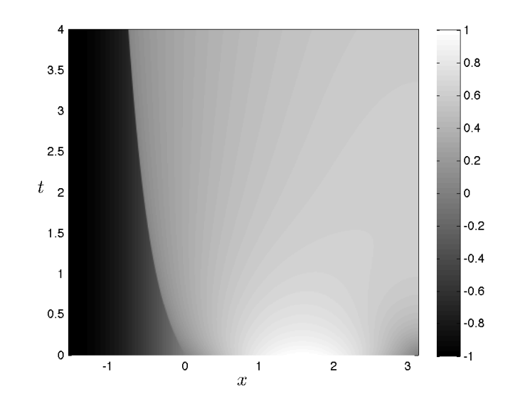
In order to simplify matters, we have chosen an example without the convective term, nevertheless a discontinuity will form in the solution due to the degeneracy of AA. This discontinuity will take the form of a boundary on which u=0u=0, moving to the left.

We have used the Euler method to integrate the system of ordinary differential equations (2.9), resulting in the update formula

uj​((n+1)​Δ​t)=uj​(n​Δ​t)+Δ​t​D−​D+​Aj​(n​Δ​t).u_{j}((n+1)\Delta t)=u_{j}(n\Delta t)+\Delta tD^{-}D^{+}A_{j}(n\Delta t).

For this to be linearly stable, the time-step Δ​t\Delta t must obey the restrictive CFL condition Δ​t≤0.5​max⁡A′​(u)​Δ​x2\Delta t\leq 0.5\max A^{\prime}(u)\Delta x^{2}.

In Figure 4.1 we show the solution in the (x,t)(x,t) plane and a snapshot of uu at t=1t=1, for an approximation using 400400 grid points in the interval (−π/2,π)(-\pi/2,\pi).

Refer to caption
Figure 4.1. An approximate solution to (4.1) using 400400 grid points. Left: uu in the (x,t)(x,t) plane for t∈[0,4]t\in[0,4]. Right: an approximation to u⁡(1,x)u(1,x) using 2525 grid points, a reference solution computed using 40004000 grid points and the initial data.

Finally we computed approximate errors, defined by

100​‖uΔ​x−uref‖L1‖uΔ​x‖L1100\frac{\left\|u_{\Delta x}-u_{\mathrm{ref}}\right\|_{L^{1}}}{\left\|u_{\Delta x}\right\|_{L^{1}}}

for a reference solution computed by using our scheme with 40004000 grid points. These errors were computed at t=1t=1. The result of this is shown in Table 4.1.

NN 2525 5050 100100 200200 400400 800800
error 3.62 1.55 0.82 0.40 0.18 0.07
rate - 1.22 0.92 1.02 1.11 1.42
Table 4.1. Numerical errors and convergence rate for the intial value problem (4.1). NN is the number of grid points.

Looking at this table, it seems the numerical rate of convergence is 11. Thus very far from the rather pessimistic lower bound proved in this paper!

References

  • [1] M. Afif and B. Amaziane. Convergence of finite volume schemes for a degenerate convection-diffusion equation arising in flow in porous media. Comput. Methods Appl. Mech. Engrg., 191(46):5265–5286, 2002.
  • [2] F. Bouchut, F. R. Guarguaglini, and R. Natalini. Diffusive BGK approximations for nonlinear multidimensional parabolic equations. Indiana Univ. Math. J., 49(2):723–749, 2000.
  • [3] M. C. Bustos, F. Concha, R. Bürger, and E. M. Tory. Sedimentation and thickening, volume 8 of Mathematical Modelling: Theory and Applications. Kluwer Academic Publishers, Dordrecht, 1999. Phenomenological foundation and mathematical theory.
  • [4] J. Carrillo. Entropy solutions for nonlinear degenerate problems. Arch. Ration. Mech. Anal., 147(4):269–361, 1999.
  • [5] G.-Q. Chen and K. H. Karlsen. L1L^{1}-framework for continuous dependence and error estimates for quasilinear anisotropic degenerate parabolic equations. Trans. Amer. Math. Soc., pages 358(3): 937–963(electronic), 2006.
  • [6] B. Cockburn and G. Gripenberg. Continuous dependence on the nonlinearities of solutions of degenerate parabolic equations. J. Differential Equations, 151(2):231–251, 1999.
  • [7] B. Cockburn and C.-W. Shu. The local discontinuous Galerkin method for time-dependent convection-diffusion systems. SIAM J. Numer. Anal., 35(6):2440–2463 (electronic), 1998.
  • [8] M. G. Crandall and A. Majda. Monotone difference approximations for scalar conservation laws. Math. Comp., 34(149):1–21, 1980.
  • [9] M. S. Espedal and K. H. Karlsen. Numerical solution of reservoir flow models based on large time step operator splitting algorithms. In Filtration in porous media and industrial application (Cetraro, 1998), volume 1734 of Lecture Notes in Math., pages 9–77. Springer, Berlin, 2000.
  • [10] S. Evje and K. H. Karlsen. Monotone difference approximation of BV solutions to degenerate convection-diffusion equations, volume 115 of Report. University of Bergen, Department of Applied Mathematics, Bergen, 1998.
  • [11] S. Evje and K. H. Karlsen. Viscous splitting approximation of mixed hyperbolic-parabolic convection-diffusion equations. Numer. Math., 83(1):107–137, 1999.
  • [12] S. Evje and K. H. Karlsen. Monotone difference approximations of BV solutions to degenerate convection-diffusion equations. SIAM J. Numer. Anal., 37(6):1838–1860 (electronic), 2000.
  • [13] S. Evje and K. H. Karlsen. An error estimate for viscous approximate solutions of degenerate parabolic equations. J. Nonlinear Math. Phys., 9(3):262–281, 2002.
  • [14] R. Eymard, T. Gallouët, and R. Herbin. Convergence of a finite volume scheme for a nonlinear hyperbolic equation. In Proceedings of the Third International Colloquium on Numerical Analysis (Plovdiv, 1994), pages 61–70, Utrecht, 1995. VSP.
  • [15] R. Eymard, T. Gallouët, and R. Herbin. Error estimate for approximate solutions of a nonlinear convection-diffusion problem. Advances in Differential Equations., pages Volume 7, No 4, 419–440, 2002.
  • [16] R. Eymard, T. Gallouët, R. Herbin, and A. Michel. Convergence of a finite volume scheme for nonlinear degenerate parabolic equations. Numerische Mathematik., pages 92: 41–82, 2002.
  • [17] A. Harten, P. D. Lax, and B. van Leer. On upstream differencing and Godunov-type schemes for hyperbolic conservation laws. SIAM Rev., 25(1):35–61, 1983.
  • [18] H. Holden, K. H. Karlsen, and K.-A. Lie. Operator splitting methods for degenerate convection-diffusion equations. I. Convergence and entropy estimates. In Stochastic processes, physics and geometry: new interplays, II (Leipzig, 1999), volume 29 of CMS Conf. Proc., pages 293–316. Amer. Math. Soc., Providence, RI, 2000.
  • [19] H. Holden, K. H. Karlsen, and N. H. Risebro. On uniqueness and existence of entropy solutions of weakly coupled systems of nonlinear degenerate parabolic equations. Electron. J. Differential Equations, pages No. 46, 31 pp. (electronic), 2003.
  • [20] K. H. Karlsen and N. H. Risebro. On the uniqueness and stability of entropy solutions of nonlinear degenerate parabolic equations with rough coefficients. Discrete Contin. Dyn. Syst., 9(5):1081–1104, 2003.
  • [21] K. H. Karlsen, N. H. Risebro, and J. D. Towers. On a nonlinear degenerate parabolic transport-diffusion equation with a discontinuous coefficient. Electron. J. Differential Equations, pages No. 93, 23 pp. (electronic), 2002.
  • [22] K. H. Karlsen, N. H. Risebro, and J. D. Towers. Upwind difference approximations for degenerate parabolic convection-diffusion equations with a discontinuous coefficient. IMA J. Numer. Anal., 22(4):623–664, 2002.
  • [23] D. Kröner and M. Rokyta. Convergence of upwind finite volume schemes for scalar conservation laws in two dimensions. SIAM J. Numer. Anal., 31(2):324–343, 1994.
  • [24] S. N. Kružkov. First order quasilinear equations with several independent variables. Mat. Sb. (N.S.), 81 (123):228–255, 1970.
  • [25] A. Kurganov and E. Tadmor. New high-resolution central schemes for nonlinear conservation laws and convection-diffusion equations. J. Comput. Phys., 160(1):241–282, 2000.
  • [26] N. N. Kuznetsov. The accuracy of certain approximate methods for the computation of weak solutions of a first order quasilinear equation. Ž. Vyčisl. Mat. i Mat. Fiz., 16(6):1489–1502, 1627, 1976.
  • [27] M. Ohlberger. A posteriori error estimates for vertex centered finite volume approximations of convection-diffusion-reaction equations. M2AN Math. Model. Numer. Anal., 35(2):355–387, 2001.
  • [28] O. A. Oleĭnik. Convergence of certain difference schemes. Soviet Math. Dokl., 2:313–316, 1961.
  • [29] S. Osher and E. Tadmor. On the convergence of difference approximations to scalar conservation laws. Math. Comp., 50(181):19–51, 1988.
  • [30] A. I. Vol′pert. Generalized solutions of degenerate second-order quasilinear parabolic and elliptic equations. Adv. Differential Equations, 5(10-12):1493–1518, 2000.
  • [31] A. I. Vol′pert and S. I. Hudjaev. The Cauchy problem for second order quasilinear degenerate parabolic equations. Mat. Sb. (N.S.), 78 (120):374–396, 1969.
  • [32] M. Westdickenberg and S. Noelle. A new convergence proof for finite volume schemes using the kinetic formulation of conservation laws. SIAM J. Numer. Anal., 37(3):742–757 (electronic), 2000.