Higher order finite difference schemes for the Magnetic Induction equations

Journal: bit

U. Koley Affiliation: E-mail: ujjwalk@cma.uio.no S. Mishra Affiliation: E-mail: siddharm@cma.uio.no N. H. Risebro Affiliation: E-mail: nilshr@math.uio.no M. Svärd Affiliation: U. Koley Affiliation: S. Mishra Affiliation: N. H. Risebro Affiliation: Centre of Mathematics for Applications (CMA)
University of Oslo
P.O. Box 1053, Blindern
N–0316 Oslo, Norway Affiliation: SINTEF ICT
Pb. 124 Blindern
N–0314 Oslo, Norway E-mail: Magnus.Svard@sintef.no

August 24, 2026

Abstract

We describe high order accurate and stable finite difference schemes for the initial-boundary value problem associated with the magnetic induction equations. These equations model the evolution of a magnetic field due to a given velocity field. The finite difference schemes are based on Summation by Parts (SBP) operators for spatial derivatives and a Simultaneous Approximation Term (SAT) technique for imposing boundary conditions. We present various numerical experiments that demonstrate both the stability as well as high order of accuracy of the schemes.

Keywords:

conservation laws induction equations summation-by-parts operators boundary conditions finite difference schemes high order of accuracy

MSC

35L65 74S10 65M12

1 Introduction

The magnetic induction equations are a special form of the Maxwell’s equations that describe the evolution of the magnetic field under the influence of a given velocity field. These equations arise in a wide variety of applications in plasma physics, astrophysics and electrical engineering. One important application are the equations of magneto-hydro dynamics (MHD). These equations combine the Euler equations of gas dynamics with the magnetic induction equations. Our goal in this paper is to describe stable and high-order accurate numerical schemes for the magnetic induction equations.

We start with a brief description of how the equations are derived. Let the magnetic field and given velocity field be denoted by ${\mathbf{B}}$ and ${\mathbf{u}}$ respectively. Faraday’s law for the magnetic flux across a surface ${\bf S}$ bounded by a curve $\partial{\bf S}$ is given by (see [18]),

\frac{d}{dt}\int\limits_{S}{\mathbf{B}}\cdot\mathbf{d}{\mathbf{S}}=\oint\limits_{\partial S}{\mathbf{E}}\cdot dl.

Using the Stokes theorem and the fact that the electric field, ${\mathbf{E}}$ , in a co-moving frame is zero and the magnetic resistivity is zero, Faraday’s law takes the form,

\frac{\partial{\mathbf{B}}}{\partial t}+{\rm div}({\mathbf{u}}\otimes{\mathbf{B}}-{\mathbf{B}}\otimes{\mathbf{u}})=-{\mathbf{u}}{\rm div}({\mathbf{B}}).

(1)

Using simple vector identities, (1) can be rewritten as,

\partial_{t}{\mathbf{B}}+\mathrm{curl}({\mathbf{B}}\times{\mathbf{u}})=-{\mathbf{u}}\mathrm{div}({\mathbf{B}}).

(2)

Magnetic monopoles have never been observed in nature. As a consequence, the magnetic field is always assumed to be divergence free, i.e., $\mathrm{div}({\mathbf{B}})=0$ . Hence, it is common to set the right-hand side of (2) to zero and couple the induction equation with the divergence constraint in order to obtain

	$\displaystyle\partial_{t}{\mathbf{B}}+\mathrm{curl}({\mathbf{B}}\times{\mathbf{u}})$	$\displaystyle=0,$		(3)
	$\displaystyle\mathrm{div}({\mathbf{B}})$	$\displaystyle=0,\,{\mathbf{B}}(x,0)={\mathbf{B}}_{0}(x).$		(3)

This form (3) is commonly used in the literature as the appropriate form of the magnetic induction equations to study and discretize. It is easy to see that (3) is hyperbolic but not strictly hyperbolic. An important tool in the analysis of hyperbolic system of equations is the derivation of energy estimates. The usual procedure in deriving energy estimates consists of symmetrizing the hyperbolic system. It is not possible to symmetrize (3) without explicitly using the divergence constraint. Hence, it is difficult to obtain energy stability starting from (3).

On the other hand, we can use the following vector identity

	$\displaystyle\mathrm{curl}({\mathbf{B}}\times{\mathbf{u}})$	$\displaystyle={\mathbf{B}}\mathrm{div}{\mathbf{u}}-{\mathbf{u}}\mathrm{div}({\mathbf{B}})+\left({\mathbf{u}}\cdot\nabla\right){\mathbf{B}}-\left({\mathbf{B}}\cdot\nabla\right){\mathbf{u}}$
		$\displaystyle=\left(u^{1}{\mathbf{B}}\right)_{x}+\left(u^{2}{\mathbf{B}}\right)_{y}+\left(u^{3}{\mathbf{B}}\right)_{z}-{\mathbf{u}}\mathrm{div}({\mathbf{B}})-({\mathbf{B}}\cdot\nabla){\mathbf{u}},$

and rewrite (1) in the non-conservative symmetric form,

	$\displaystyle\partial_{t}{\mathbf{B}}+\left({\mathbf{u}}\cdot\nabla\right){\mathbf{B}}$	$\displaystyle=-{\mathbf{B}}(\mathrm{div}{\mathbf{u}})+({\mathbf{B}}\cdot\nabla){\mathbf{u}}$		(4)
		$\displaystyle=M(D{\mathbf{u}}){\mathbf{B}},$		(4)

where the $D{\mathbf{u}}$ denotes the gradient of ${\mathbf{u}}$ and the matrix $M(D{\mathbf{u}})$ is given by

M(D{\mathbf{u}})=\begin{pmatrix}-\partial_{y}u^{2}-\partial_{z}u^{3}&\partial_{y}u^{1}&\partial_{z}u^{1}\\ \partial_{x}u^{2}&-\partial_{x}u^{1}-\partial_{z}u^{3}&+\partial_{z}u^{2}\\ \partial_{x}u^{3}&\partial_{y}u^{3}&-\partial_{x}u^{1}-\partial_{y}u^{2}\end{pmatrix}.

Introducing the matrix,

C=-\begin{pmatrix}\partial_{x}u^{1}&\partial_{y}u^{1}&\partial_{z}u^{1}\\ \partial_{x}u^{2}&\partial_{y}u^{2}&\partial_{z}u^{2}\\ \partial_{x}u^{3}&\partial_{y}u^{3}&\partial_{z}u^{1}\end{pmatrix},

(1) can also be written in the following “conservative” symmetric form,

\partial_{t}{\mathbf{B}}+\partial_{x}\left(A^{1}{\mathbf{B}}\right)+\partial_{y}\left(A^{2}{\mathbf{B}}\right)+\partial_{z}\left(A^{3}{\mathbf{B}}\right)+C{\mathbf{B}}=0,

(5)

where $A^{i}=u^{i}I$ for $i=1,2,3$ . Note that the symmetrized matrices in (5) are diagonal and that the only coupling in the equations is through the lower order terms. These symmetrized forms are in the same spirit as the non-linear symmetrized forms of MHD equations introduced in [8].

Furthermore, by taking divergence on both sides of (2) we get

(\mathrm{div}({\mathbf{B}}))_{t}+\mathrm{div}\left({\mathbf{u}}\mathrm{div}({\mathbf{B}})\right)=0.

(6)

Hence, if $\mathrm{div}({\mathbf{B}}_{0}({\mathbf{x}}))=0$ , also $\mathrm{div}({\mathbf{B}}({\mathbf{x}},t))=0$ for $t>0$ . This implies that all the above forms (5), and (3) are equivalent (at least for smooth solutions). Introducing the space $H^{\mathrm{div}}$ as

H^{\mathrm{div}}(\mathbb{R}^{3})=\left\{\mathbf{w}:\mathbb{R}^{3}\to\mathbb{R}^{3}\;\bigm|\;\left|\mathbf{w}\right|\in L^{2}(\mathbb{R}^{3}),\;\;\mathrm{div}(\mathbf{w})\in L^{2}(\mathbb{R}^{3})\right\},

we have the following theorem:

Theorem 1.1

Assume that the velocity field ${\mathbf{u}}$ is sufficiently smooth, and that ${\mathbf{B}}_{0}\in H^{\mathrm{div}}(\mathbb{R}^{3})$ . Then there exists a unique weak solution ${\mathbf{B}}\in C([0,T];H^{\mathrm{div}}(\mathbb{R}^{3}))$ of (5). The solution ${\mathbf{B}}$ satisfies the energy estimate,

\left\|{\mathbf{B}}(\cdot,T)\right\|_{H^{\mathrm{div}}(\mathbb{R}^{3})}\leq C_{T}\left\|{\mathbf{B}}_{0}\right\|_{H^{\mathrm{div}}(\mathbb{R}^{3})}

The constant $C_{T}$ depends only on the final time $T$ . Furthermore, if $\mathrm{div}({\mathbf{B}}_{0})=0$ , then the physical form (1) and the symmetric form (5) are equivalent to the constrained form (3), i.e., ${\mathbf{B}}$ is also the unique weak solution of (3).

The proof of the above theorem uses the energy estimate and we will provide a sketch of the proof for the two-dimensional version of the equations together with boundary conditions later in this paper.

Even though the magnetic induction equations are linear, the presence of variable coefficients and lower order terms means that general closed form solutions are not available. Hence, one has to design suitable numerical schemes for these equations. Furthermore, since these equations appear as a sub-model in the MHD equations, the design of stable and high-order accurate numerical schemes for the induction equations can lead to the design of robust schemes for the non-linear MHD equations.

Most of the attention in the literature has been focused on the constrained form (3). The key issue in the design of a suitable numerical scheme to approximate (3) has been the treatment of the divergence constraint. A widely used approach has been to employ projection methods based on a Hodge decomposition of the magnetic field. A base (finite difference or finite volume) scheme is used to evolve the magnetic field. The evolved field, which need not be divergence free, is then corrected for divergence errors by solving an elliptic equation (see [3]). The resulting method is computationally expensive, as the elliptic equation has to be solved at every time step.

Another common approach is to discretize (3) such that some particular form of discrete divergence is preserved at each time step (see [23]). This approach is equivalent to staggering the velocity and magnetic fields in each direction (see [4, 1, 20, 5] and a detailed comparison in [24]). Some of these schemes are proved to be von Neumann stable in the special case of constant velocity fields. No stability analysis is available either in the case of variable velocity fields or for problems with boundary conditions. These schemes also involve wider stencils than what is required for a standard finite difference scheme.

Despite all the attempts at finding a suitable discretization of (3) and preserving a special form of discrete divergence, it is not clear as to whether such an approach is appropriate. Furthermore, there are many different choices for the discrete divergence operator and preserving some form of discrete divergence exactly does not lead to preservation or even keeping divergence errors small for a different form. The main aim should be to design a stable scheme to approximate magnetic fields and it is not clear whether preserving divergence in a particular discrete form helps. One reason for the difficulties in proving stability of discretizations for (3) with general velocity fields may lie in the very form of these equations. As remarked earlier, (3) are not symmetrizable directly and thus one cannot obtain energy estimates in this form. This remains true for discretizations of (3).

A different approach consisting of discretizing the physical form (1) was proposed in [17] for the non-linear MHD equations. Adapting this to (1) implies using a standard upwind scheme for the convection part and a centered discretization of the source terms. From (6), one can expect that divergence errors will be transported out of the domain for transparent boundary conditions. This approach does not imply stability either and can lead to oscillations as reported in [6]. A discontinuous Galerkin based discretization of the symmetric form (5) was proposed in [2].

In a recent paper [6], the authors discretized the symmetric form (4) by using a first order accurate upwind finite difference scheme. The resulting scheme also implied an upwind discretization of the convection term in (1) with an upwind discretization of the source term. This scheme was shown to be energy stable even with variable velocity fields and to be TVD for constant velocity fields.

Furthermore, boundary conditions were not considered either in [6] or any of the aforementioned papers. High-order accurate schemes will lead to much better resolution of interesting solution features and a stable discretization of the boundary conditions (while still preserving high order of accuracy) is desirable.

Our aim in this paper is to design stable and high-order accurate schemes for initial-boundary value problems corresponding to the magnetic induction equations by discretizing the non-conservative symmetric form (4). The spatial derivatives are approximated by second and fourth-order SBP (Summation-By-Parts) operators. The boundary conditions are weakly imposed by using a SAT (Simultaneous Approximation Term) and time integration is performed by standard Runge-Kutta schemes. The SBP-SAT framework has been used to obtain stable and accurate high order schemes for a wide variety of hyperbolic problems in recent years. See [22] and the references therein for more details.

The SBP-SAT schemes use centered finite difference stencils in the interior, which lead to oscillations in the vicinity of discontinuities. We apply well-known SBP-SAT compatible numerical diffusion operators in case of discontinuous data.

The rest of this paper is organized as follows: In Section 2, we state the energy estimate for the initial-boundary value problem corresponding to (4) in order to motivate the proof of stability for the scheme. In Section 3, we present the SBP-SAT scheme and show stability. Numerical experiments are presented in Section 4 and conclusions are drawn in Section 5.

2 The Continuous problem

For ease of notation, we shall restrict ourselves to two spatial dimensions in the remainder of this paper. Extending the results to three dimensions is straightforward.

In two dimensions, the non-conservative symmetric form (4) reads

\displaystyle{\mathbf{B}}_{t}+\Lambda_{1}{\mathbf{B}}_{x}+\Lambda_{2}{\mathbf{B}}_{y}-C{\mathbf{B}}

\displaystyle=0,

(7)

where

\displaystyle\Lambda_{1}

\displaystyle=\begin{pmatrix}u^{1}&0\\ 0&u^{1}\end{pmatrix},\quad\Lambda_{2}=\begin{pmatrix}u^{2}&0\\ 0&u^{2}\end{pmatrix},\quad C=\begin{pmatrix}-\partial_{y}u^{2}&\partial_{y}u^{1}\\ \partial_{x}u^{2}&-\partial_{x}u^{1}\end{pmatrix},

with ${\mathbf{B}}=\left(B^{1},B^{2}\right)^{T}$ and ${\mathbf{u}}=\left(u^{1},u^{2}\right)^{T}$ denoting the magnetic and velocity fields respectively. In component form, (7) becomes

	$\displaystyle(B^{1})_{t}+u^{1}(B^{1})_{x}+u^{2}(B^{1})_{y}$	$\displaystyle=-(u^{2})_{y}B^{1}+(u^{1})_{y}B^{2}$		(8)
	$\displaystyle(B^{2})_{t}+u^{1}(B^{2})_{x}+u^{2}(B^{2})_{y}$	$\displaystyle=(u^{2})_{x}B^{1}-(u^{1})_{x}B^{2}.$		(8)

To begin with, we shall consider (7) in the domain $(x,y)\in\Omega=[0,1]^{2}$ .

We augment (7) with initial conditions,

\displaystyle{\mathbf{B}}({\mathbf{x}},0)={\mathbf{B}}_{0}({\mathbf{x}})\quad{\mathbf{x}}\in\Omega,

(9)

and Dirichlet boundary conditions,

	$\displaystyle\mathbf{1}_{\left\{u^{1}(0,y,t)>0\right\}}\Bigl({\mathbf{B}}(0,y,t)$	$\displaystyle={\mathbf{g}}(0,y,t)\Bigr),\quad\mathbf{1}_{\left\{u^{1}(1,y,t)<0\right\}}\Bigl({\mathbf{B}}(1,y,t)={\mathbf{g}}(1,y,t)\Bigr),$		(10)
	$\displaystyle\mathbf{1}_{\left\{u^{2}(x,0,t)>0\right\}}\Bigl({\mathbf{B}}(x,0,t)$	$\displaystyle={\mathbf{g}}(x,0,t)\Bigr),\quad\mathbf{1}_{\left\{u^{2}(x,1,t)<0\right\}}\Bigl({\mathbf{B}}(x,1,t)={\mathbf{g}}(x,1,t)\Bigr)$		(10)

where $\mathbf{1}_{A}$ denotes the characteristic function of the set $A$ . Note that we only impose boundary conditions on the set where the characteristics are entering the domain.

Definition 1

Weak solution: A function ${\mathbf{B}}:\Omega\to\mathbb{R}^{2}$ such that ${\mathbf{B}}\in C([0,T];H^{1}(\Omega))$ is defined as a weak solution of (7) with initial data (9) and boundary data (10) if it satisfies the weak formulation of (7) in $\Omega$ , i.e.,

\int_{0}^{T}\int_{\Omega}{\mathbf{B}}\left(\varphi_{t}+\left(\Lambda_{1}\varphi\right)_{x}+\left(\Lambda_{2}\varphi\right)_{y}-C\varphi\right)\,dxdydt+\int_{\Omega}{\mathbf{B}}_{0}\varphi(x,y,0)\,dxdy\\ -\int_{0}^{T}\int_{0}^{1}u^{1}\left(Tr{\mathbf{B}}\right)\varphi(x,y,t)\bigm|^{x=1}_{x=0}\,dydt-\int_{0}^{T}\int_{0}^{1}u^{2}\left(Tr{\mathbf{B}}\right)\varphi(x,y,t)\bigm|^{y=1}_{y=0}\,dxdt=0,

(11)

for all test functions $\varphi\in C^{\infty}_{0}(\Omega\times[0,T))$ . By $Tr{\mathbf{B}}$ we mean the $H^{1}$ trace of ${\mathbf{B}}$ at the boundary. The boundary conditions (10) are taken in the sense of $H^{1}$ traces.

We shall always assume that the initial and boundary data satisfy the compatibility conditions, i.e., specific criteria that guarantee smoothness of the solution, see [9].

Theorem 2.1

Assume that ${\mathbf{B}}_{0}\in H^{1}(\Omega)$ , that ${\mathbf{g}}\in H^{1}(\partial\Omega\times[0,T])$ for $T>0$ and that $u^{1}$ and $u^{2}$ are in $H^{2}(\Omega\times[0,T])$ . Then there exists a function ${\mathbf{B}}\in C([0,T],L^{2}(\Omega))\cap L^{\infty}([0,T];H^{1}(\Omega))$ which is the unique weak solution of (7) with the initial and boundary conditions (9) and (10).

Furthermore, it satisfies the following stability estimate

\left\|{\mathbf{B}}(\cdot,t)\right\|_{H^{1}(\Omega)}^{2}\leq e^{\alpha t}\left(\left\|{\mathbf{B}}_{0}\right\|_{H^{1}(\Omega)}^{2}+\left\|{\mathbf{g}}\right\|_{H^{1}(\partial\Omega\times(0,t))}\right).

(12)

where $\alpha$ is a positive constant.

Proof

The proof of this theorem is standard. Assume first that ${\mathbf{g}}$ , ${\mathbf{B}}_{0}$ and ${\mathbf{u}}$ are in $C^{\infty}$ . Since the compatibility conditions are satisfied, a unique solution exists by the method of characteristics. Let $\left(a\vee 0\right)=\max\left\{a,0\right\}$ and $\left(a\wedge 0\right)=\min\left\{a,0\right\}$ . Multiplying the equation by ${\mathbf{B}}$ and integrating over $\Omega$ yields

		$\displaystyle\qquad\frac{d}{dt}\int_{\Omega}{\mathbf{B}}^{T}{\mathbf{B}}\,dxdy$
		$\displaystyle=\int_{\Omega}{\mathbf{B}}\left(2C+\mathrm{div}({\mathbf{u}})\right){\mathbf{B}}\,dxdy-\int_{0}^{1}u^{1}Tr({\mathbf{B}}^{T}{\mathbf{B}})\bigm\|^{x=1}_{x=0}\,dy+\int_{0}^{1}u^{2}Tr({\mathbf{B}}^{T}{\mathbf{B}})\bigm\|^{y=1}_{y=0}\,dx$
		$\displaystyle\leq c\int_{\Omega}{\mathbf{B}}^{T}{\mathbf{B}}\,dxdy$
		$\displaystyle\qquad+\int_{0}^{1}\left(u^{1}(0,y,t)\vee 0\right)\left(Tr({\mathbf{B}}^{T}{\mathbf{B}})\right)\,dy-\int_{0}^{1}\left(u^{1}(1,y,t)\wedge 0\right)\left(Tr({\mathbf{B}}^{T}{\mathbf{B}})\right)\,dy$
		$\displaystyle\qquad+\int_{0}^{1}\left(u^{2}(x,0,t)\vee 0\right)\left(Tr({\mathbf{B}}^{T}{\mathbf{B}})\right)\,dx-\int_{0}^{1}\left(u^{2}(x,1,t)\wedge 0\right)\left(Tr({\mathbf{B}}^{T}{\mathbf{B}})\right)\,dx$
		$\displaystyle\leq c\biggl(\int_{\Omega}({\mathbf{B}}^{T}{\mathbf{B}})\,dxdy+\int_{\partial\Omega}{\mathbf{g}}^{2}\,ds\biggr)$

for some constant $c$ depending on ${\mathbf{u}}$ and its first derivatives. Via the Grönwall inequality we get the bound

\left\|{\mathbf{B}}(\cdot,t)\right\|_{L^{2}(\Omega)}^{2}\leq e^{ct}\left(\left\|{\mathbf{B}}_{0}\right\|_{L^{2}(\Omega)}^{2}+\int_{0}^{T}\int_{\partial\Omega}{\mathbf{g}}^{2}\,ds\,dt\right).

Set ${\mathbf{P}}={\mathbf{B}}_{x}$ and ${\mathbf{Q}}={\mathbf{B}}_{y}$ , applying $\partial_{x}$ to (7) yields

{\mathbf{P}}_{t}+u^{1}{\mathbf{P}}_{x}+u^{2}{\mathbf{P}}_{y}=u^{1}_{x}{\mathbf{P}}+u^{2}_{x}{\mathbf{Q}}+C{\mathbf{P}}+C_{x}{\mathbf{B}}.

(13)

Furthermore, $P(x,y,0)=\partial_{x}{\mathbf{B}}_{0}(x,y)$ and at those parts of $\partial\Omega$ where we impose boundary data

	$\displaystyle u^{1}{\mathbf{P}}$	$\displaystyle=C{\mathbf{g}}-{\mathbf{g}}_{t}-u^{2}{\mathbf{g}}_{y}\quad\text{on $x=0$ and $x=1$,}$
	$\displaystyle u^{2}{\mathbf{Q}}$	$\displaystyle=C{\mathbf{g}}-{\mathbf{g}}_{t}-u^{2}{\mathbf{g}}_{x}\quad\text{on $y=0$ and $y=1$.}$

We shall also be needing ${\mathbf{P}}$ on $y=0$ and $1$ and ${\mathbf{Q}}$ on $x=0$ and $1$ . These are given by ${\mathbf{g}}_{x}$ and ${\mathbf{g}}_{y}$ respectively.

Multiplying (13) with $2{\mathbf{P}}^{T}$ and rearranging yields

{\mathbf{P}}^{2}_{t}+\left(u^{1}{\mathbf{P}}^{2}\right)_{x}+\left(u^{2}{\mathbf{P}}^{2}\right)_{y}=-u^{1}_{x}{\mathbf{P}}^{2}-2u^{2}_{x}{\mathbf{P}}^{T}{\mathbf{Q}}+2{\mathbf{P}}^{T}C{\mathbf{P}}+2{\mathbf{P}}^{T}C_{x}{\mathbf{B}}.

We also have an analogous equation for ${\mathbf{Q}}^{2}$ ;

{\mathbf{Q}}^{2}_{t}+\left(u^{1}{\mathbf{Q}}^{2}\right)_{x}+\left(u^{2}{\mathbf{Q}}^{2}\right)_{y}=-u^{2}_{y}{\mathbf{Q}}^{2}-2u^{1}_{y}{\mathbf{P}}^{T}{\mathbf{Q}}+2{\mathbf{P}}^{T}C{\mathbf{Q}}+2{\mathbf{Q}}^{T}C_{y}{\mathbf{B}}.

Adding these two equations we find

\left({\mathbf{P}}^{2}+{\mathbf{Q}}^{2}\right)_{t}+\left(u^{1}\left({\mathbf{P}}^{2}+{\mathbf{Q}}^{2}\right)\right)_{x}+\left(u^{2}\left({\mathbf{P}}^{2}+{\mathbf{Q}}^{2}\right)\right)_{y}=R,

(14)

where by Hölder’s inequality $R$ has the bound

\int_{\Omega}R(x,y,t)\,dxdy\leq c\left(\left\|{\mathbf{B}}(\cdot,t)\right\|_{L^{2}(\Omega)}^{2}+\left\|{\mathbf{P}}(\cdot,t)\right\|_{L^{2}(\Omega)}^{2}+\left\|{\mathbf{Q}}(\cdot,t)\right\|_{L^{2}(\Omega)}^{2}\right),

where the constant $c$ depends on ${\mathbf{u}}$ and its derivatives. By reasoning as we did with ${\mathbf{B}}$ , we can then get the bound

\frac{d}{dt}\left(\left\|{\mathbf{P}}\right\|_{L^{2}(\Omega)}^{2}+\left\|{\mathbf{Q}}\right\|_{L^{2}(\Omega)}^{2}\right)\leq\\ c\left(\left\|{\mathbf{B}}(\cdot,t)\right\|_{L^{2}(\Omega)}^{2}+\left\|{\mathbf{P}}\right\|_{L^{2}(\Omega)}^{2}+\left\|{\mathbf{Q}}\right\|_{L^{2}(\Omega)}^{2}+\int_{\partial\Omega}{\mathbf{g}}_{t}^{2}+{\mathbf{g}}_{x}^{2}+{\mathbf{g}}_{y}^{2}\,ds\right).

Via Grönwall’s inequality and the bounds on $\left\|{\mathbf{B}}\right\|_{L^{2}}$ we find

\left\|{\mathbf{P}}(\cdot,t)\right\|_{L^{2}(\Omega)}^{2}+\left\|{\mathbf{Q}}(\cdot,t)\right\|_{L^{2}(\Omega)}^{2}\leq\mathrm{Const.},

where the constant depends on the $H^{1}(\Omega)$ norm of ${\mathbf{B}}_{0}$ and ${\mathbf{g}}$ and on ${\mathbf{u}}$ and its derivatives. This means that we have an energy estimate

\left\|{\mathbf{B}}(\cdot,t)\right\|_{H^{1}(\Omega)}\leq C_{t}\left(\left\|{\mathbf{B}}_{0}\right\|_{H^{1}(\Omega)}+\left\|{\mathbf{g}}\right\|_{H^{1}(\partial\Omega\times(0,t))}\right),

where $C_{t}$ is a finite constant depending on $t$ , ${\mathbf{u}}$ and its derivatives.

Then, for a general initial data, velocity fields and boundary conditions, we can use a standard approximation argument ([10]) and the above estimate to pass to the limit and prove the existence and uniqueness of weak solutions.

Remark 1

The above theorem has been proved in the unit square. It can be easily extended to domains with smooth (i.e., $C^{1}$ boundaries) by using cut-off functions and mappings between the domain and the upper-half space. See [19] and other references therein for details.

3 Semi-discrete Schemes

As stated before, we will approximate (7) with SBP-SAT finite difference schemes. We start by defining a SBP operator approximating the first derivative of a continuous function $w(x)$ in one space dimension. Let $\left\{x_{i}\right\}_{i=0}^{n}$ be equidistant points in $[0,1]$ such that $x_{i}=ih$ where $h=1/n$ . We organize the values of $w$ at $\left\{x_{i}\right\}$ in a vector $w^{T}(t)=(w_{0},...,w_{n})$ where $w_{i}=w(x_{i})$ . Then , we define,

Definition 2

A difference approximation (given by a $(n+1)\times(n+1)$ matrix $D$ ) for the first derivative is called a Summation-By-Parts (SBP) operator if $D=P^{-1}Q$ for $n\times n$ matrices $P$ and $Q$ , where $P>0$ , $P=P^{T}$ and $Q+Q^{T}=\mathcal{B}=\mathrm{diag}(-1,0,0,\ldots,0,0,1)$ .

Moreover, $P$ must define a scalar product $(w,v)=w^{T}Pv$ for which the corresponding norm, $\left\|w\right\|^{2}_{P}=(w,w)$ , is equivalent to the standard $l^{2}$ -norm, $\left\|w\right\|_{2}^{2}=h\sum_{i=1}^{n}w_{i}^{2}$ .

SBP operators of different orders of accuracy are presented in several papers, see the references in e.g. [22]. To discretize (7), we introduce equidistant meshes in the $x$ and $y$ directions with $N$ and $M$ mesh points and $\Delta x=1/N$ and $\Delta y=1/M$ . The discrete solution consists of a column vector of length $2(N+1)(M+1)$ denoted $V=(V^{1},V^{2})^{T}$ , where $V^{\ell}$ is a vector of length $(N+1)(M+1)$ ordered as

V^{\ell}=\left(V^{\ell}_{0,0},V^{\ell}_{0,1},\ldots,V^{\ell}_{0,N},V^{\ell}_{1,0},\ldots,\ldots,V^{\ell}_{N,M}\right).

and $V^{\ell}_{i,j}$ is the discrete solution at $(x_{i},y_{j})$ for $\ell=1,\,2$ . We will use the norm

\left\|w\right\|_{P}^{2}=w^{T}(P_{x}\otimes P_{y})w

where we have introduced the Kronecker product, which is defined as follows:

Let $A$ and $C$ be $n\times n$ matrices and $B$ and $D$ be $m\times m$ matrices. Then $A\otimes B$ is the $nm\times nm$ matrix

(A\otimes B)=\begin{pmatrix}a_{11}B&\ldots&a_{1n}B\\ \vdots&\ddots&\vdots\\ a_{n1}B&\ldots&a_{nn}B\end{pmatrix}.

Furthermore, the following rules hold; $(A\otimes B)(C\otimes D)=(AC\otimes BD)$ , $(A\otimes B)+(C\otimes D)=(A+C)\otimes(B+D)$ and $(A\otimes B)^{T}=(A^{T}\otimes B^{T})$ .

To define discrete boundary conditions, we need some further notation. For real numbers $\sigma_{i}$ , introduce the $2\times 2$ matrices

\displaystyle\Sigma_{0,y}=\sigma_{1}I_{2},\quad\Sigma_{N,y}=\sigma_{2}I_{2},\quad\Sigma_{x,0}=\sigma_{3}I_{2},\quad\Sigma_{x,N}=\sigma_{4}I_{2},

where the $I_{2}$ is the $2\times 2$ identity matrix and the numbers $\sigma_{i}$ are to be determined later. We also need $(M+1)\times(M+1)$ matrices $F_{0,y}$ and $F_{N,y}$

	$\displaystyle F_{0,y}$	$\displaystyle=\begin{pmatrix}1&0&\cdot&\cdot&\cdot&0\\ 0&\cdot&\cdot&\cdot&\cdot&0\\ \cdot&\cdot&\cdot&\cdot&\cdot&\cdot\\ 1&0&\cdot&\cdot&\cdot&0\\ 0&\cdot&\cdot&\cdot&\cdot&0\\ \cdot&\cdot&\cdot&\cdot&\cdot&\cdot\end{pmatrix},\quad F_{N,y}=\begin{pmatrix}0&\cdot&\cdot&\cdot&\cdot&1\\ 0&\cdot&\cdot&\cdot&\cdot&0\\ \cdot&\cdot&\cdot&\cdot&\cdot&\cdot\\ 0&\cdot&\cdot&\cdot&\cdot&1\\ 0&\cdot&\cdot&\cdot&\cdot&0\\ \cdot&\cdot&\cdot&\cdot&\cdot&\cdot\end{pmatrix},$
and $(N+1)\times(N+1)$ matrices $F_{x,0}$ and $F_{x,M}$ ,
	$\displaystyle F_{x,0}$	$\displaystyle=\begin{pmatrix}1&0&\cdot&\cdot&\cdot&0\\ 0&\cdot&\cdot&\cdot&\cdot&0\\ \cdot&\cdot&\cdot&\cdot&\cdot&\cdot\\ 1&0&\cdot&\cdot&\cdot&0\\ 0&\cdot&\cdot&\cdot&\cdot&0\\ \cdot&\cdot&\cdot&\cdot&\cdot&\cdot\end{pmatrix},\quad F_{x,M}=\begin{pmatrix}0&\cdot&\cdot&\cdot&\cdot&1\\ 0&\cdot&\cdot&\cdot&\cdot&0\\ \cdot&\cdot&\cdot&\cdot&\cdot&\cdot\\ 0&\cdot&\cdot&\cdot&\cdot&1\\ 0&\cdot&\cdot&\cdot&\cdot&0\\ \cdot&\cdot&\cdot&\cdot&\cdot&\cdot\end{pmatrix}.$

Next set

\displaystyle E_{0,y}=I_{x}\otimes F_{0,y},\quad E_{N,y}=I_{x}\otimes F_{N,y},\quad E_{x0}=F_{x,0}\otimes I_{y},\quad\text{and}\quad E_{x,M}=F_{x,M}\otimes I_{y}

where $I_{x}$ and $I_{y}$ are $(N+1)\times(N+1)$ and $(M+1)\times(M+1)$ identity matrices respectively and define

	$\displaystyle\Lambda_{x}$	$\displaystyle=I_{2}\otimes\mathrm{diag}\left(u^{1}_{0,0},u^{1}_{0,1},\ldots,u^{1}_{0,N},u^{1}_{1,0},\ldots,\ldots,u^{1}_{N,M}\right)$
	$\displaystyle\Lambda_{y}$	$\displaystyle=I_{2}\otimes\mathrm{diag}\left(u^{2}_{0,0},u^{2}_{0,1},\ldots,u^{2}_{0,N},u^{2}_{1,0},\ldots,\ldots,u^{2}_{N,M}\right).$

Define the matrix $C$ by,

\displaystyle C=\begin{pmatrix}-\left(I_{x}\otimes\left(P_{y}^{-1}Q_{y}\right)\right)u^{2}&\left(I_{x}\otimes\left(P_{y}^{-1}Q_{y}\right)\right)u^{1}\\ \left(\left(P_{x}^{-1}Q_{x}\right)\otimes I_{y}\right)u^{2}&-\left(\left(P_{x}^{-1}Q_{x}\right)\otimes I_{y}\right)u^{1}\end{pmatrix}.

Let $g$ be a column vector of the same length as $V$ , where we store the boundary values at the appropriate places. Then we can describe the SBP-SAT scheme as

$\displaystyle\partial_{t}$	$\displaystyle V+\Lambda_{x}\left(I_{2}\otimes\left(P_{x}^{-1}Q_{x}\right)\otimes I_{y}\right)V+\Lambda_{y}\left(I_{2}\otimes I_{x}\otimes\left(P_{y}^{-1}Q_{y}\right)\right)V+CV$	(15)
	$\displaystyle=\Sigma_{0,y}\otimes\left(P_{x}^{-1}\otimes I_{y}\right)\otimes E_{0y}\left(V-g\right)+\Sigma_{Ny}\otimes\left(P_{x}^{-1}\otimes I_{y}\right)\otimes E_{N,y}\left(V-g\right)$
	$\displaystyle+\Sigma_{x0}\otimes\left(I_{x}\otimes P_{y}^{-1}\right)\otimes E_{x0}\left(V-g\right)+\Sigma_{x,N}\otimes\left(I_{x}\otimes P_{y}^{-1}\right)\otimes E_{xN}\left(V-g\right),$

Theorem 3.1

Assume that the velocity field ${\mathbf{u}}$ is a constant given by ${\mathbf{u}}=(u^{1},u^{2})^{T}$ , and let $V$ be the semi-discrete solution defined by the scheme (15). Let $u^{\ell,+}=\left(u^{\ell}\vee 0\right)$ and $u^{\ell,-}=\left(u^{\ell}\wedge 0\right)$ , for $\ell=1,\>2$ . If the penalty parameters satisfy

\begin{gathered}\sigma_{1}\leq-\frac{u^{1,+}}{2},\ \sigma_{2}\leq-\frac{u^{1,-}}{2},\ \sigma_{3}\leq\frac{u^{2,+}}{2}\ \quad{\rm and}\quad\sigma_{4}\leq\frac{u^{2,-}}{2}\end{gathered}

(16)

there exists positive constants $\alpha$ and $K$ such that

\left\|V(t)\right\|^{2}\leq\left\|{\mathbf{B}}_{0}\right\|^{2}+\int\limits_{0}^{t}\int_{\partial\Omega}{\mathbf{g}}(t,x)\,dxd\tau,

(17)

and the scheme (15) is stable.

Proof

The proof is similar to the standard way of proving stability of SBP-SAT schemes (see [22]) and follows the proof for obtaining energy stability of the continuous problem in theorem 2.1. We outline the proof for the sake of completeness. For simplicity, we consider the case of constant velocities by setting $C=0$ in (15) We start by multiplying (15) with $V^{T}(I_{2}\otimes P_{x}\otimes P_{y})$ to obtain,

$\displaystyle V^{T}$	$\displaystyle\left(I_{2}\otimes P_{x}\otimes P_{y}\right)\partial_{t}V$	(18)
	$\displaystyle=-V^{T}\left(\Lambda_{x}\otimes Q_{x}\otimes P_{y}\right)V+V^{T}\left(\Lambda_{y}\otimes P_{x}\otimes Q_{y}\right)V$
	$\displaystyle+V^{T}(I_{2}\otimes P_{x}\otimes P_{y})\otimes\left[\begin{aligned} &\left(\Sigma_{0y}\otimes P_{x}^{-1}\otimes I_{y}\right)E_{0,y}+\left(\Sigma_{N,y}\otimes P_{x}^{-1}\otimes I_{y}\right)E_{N,y}\\ &\;+(\Sigma_{x,0}\otimes I_{x}\otimes P_{y}^{-1})E_{x,0}+(\Sigma_{x,N}\otimes I_{x}\otimes P_{y}^{-1})E_{x,M}\end{aligned}\right]V.$

Adding this to its transpose and using the definition of SBP operators, we obtain

	$\displaystyle\frac{d}{dt}$	$\displaystyle\left\\|V\right\\|^{2}$
		$\displaystyle=-V^{T}\left(\Lambda_{1}\otimes\mathcal{B}_{x}\otimes P_{y}\right)V+V^{T}\left(\Lambda_{2}\otimes P_{x}\otimes\mathcal{B}_{y}\right)V$
		$\displaystyle\quad+2V^{T}(I_{2}\otimes P_{x}\otimes P_{y})\otimes\left[\begin{aligned} &\left(\Sigma_{0,y}\otimes P_{x}^{-1}\otimes I_{y}\right)E_{0,y}+\left(\Sigma_{N,y}\otimes P_{x}^{-1}\otimes I_{y}\right)E_{N,y}\\ &\;+\left(\Sigma_{x,0}\otimes I_{x}\otimes P_{y}^{-1}\right)E_{x,0}+\left(\Sigma_{x,N}\otimes I_{x}\otimes P_{y}^{-1}\right)E_{x,N}\end{aligned}\right]V,$

which implies

	$\displaystyle\frac{d}{dt}\left\\|V\right\\|^{2}$	$\displaystyle=u^{1}\left(V^{1}_{0,y}\right)^{T}P_{y}\left(V^{1}_{0,y}\right)-u^{1}\left(V^{1}_{N,y}\right)^{T}P_{y}\left(V^{1}_{N,y}\right)+u^{1}\left(V^{2}_{0,y}\right)^{T}P_{y}\left(V^{2}_{0,y}\right)$
		$\displaystyle\quad-u^{1}\left(V^{2}_{N,y}\right)^{T}P_{y}\left(V^{2}_{N,y}\right)+u^{2}\left(V^{1}_{x,0}\right)^{T}P_{x}\left(V^{1}_{x,0}\right)-u^{2}\left(V^{1}_{x,M}\right)^{T}P_{x}\left(V^{1}_{x,M}\right)$
		$\displaystyle\quad+u^{2}\left(V^{2}_{x,0}\right)^{T}P_{x}\left(V^{2}_{x,0}\right)-u^{2}\left(V^{2}_{x,N}\right)^{T}P_{x}\left(V^{2}_{x,N}\right)$
		$\displaystyle\quad+2\Bigl[\sigma_{1}\left(\left(V^{1}_{0,y}\right)^{T}P_{y}\left(V^{1}_{0y}\right)+\left(V^{2}_{0,y}\right)^{T}P_{y}\left(V^{2}_{0,y}\right)\right)+\sigma_{2}\left(V^{1}_{N,y}\right)^{T}P_{y}\left(V^{1}_{N,y}\right)$
		$\displaystyle\hphantom{\quad+ 2 \Bigl[}\quad+\sigma_{2}\left(V^{2}_{N,y}\right)^{T}P_{y}\left(V^{2}_{N,y}\right)+\sigma_{3}\left(\left(V^{1}_{x,0}\right)^{T}P_{x}\left(V^{1}_{x,0}\right)+\left(V^{2}_{x,0}\right)^{T}P_{x}\left(V^{2}_{x,0}\right)\right)$
		$\displaystyle\hphantom{\quad+ 2 \Bigl[}\quad+\sigma_{4}\left(\left(V^{1}_{x,N}\right)^{T}P_{x}\left(V^{1}_{x,N}\right)\left(V^{2}_{x,N}\right)^{T}P_{x}\left(V^{2}_{x,N}\right)\right)\Bigr].$

Using (16) and integrating in time gives the energy estimate (17).

Remark 2

The above proof of stability assumes a constant velocity field. A proof of stability with a general velocity fields has been obtained in a recent paper [14] by using the principle of frozen coefficients. The resulting stability estimate will lead to an exponential growth of energy (similar to (12)) due to the presence of lower order terms.

We conclude this section with a few comments. For simplicity, we have only considered Cartesian meshes. However, the proofs are readily generalized to curvilinear grids by transforming the domain to a Cartesian. A stability proof is then obtained by freezing the coefficients. However, that requires $P$ to be diagonal, [21]. Furthermore, multi-block grids can also be handled and stable interfaces derived in a similar way as in, [16].

4 Numerical Experiments

We test the SBP-SAT schemes of the previous section on a suite of numerical experiments in order to demonstrate the effectiveness of these schemes. We will use two different schemes : $SBP2$ and $SBP4$ scheme which are second-order (first-order) and fourth order (second-order) accurate in the interior (boundary) resulting in an overall second and third-order of accuracy. Time integration is performed by using a second order accurate Runge-Kutta scheme at a $CFL$ number of $0.45$ for all numerical experiments. We found that using a fourth order accurate Runge-Kutta scheme resulted in negligible differences in the numerical results. The schemes have bounded errors, a typical behavior for hyperbolic equations with characteristic boundary conditions as shown in [15]. Errors are propagated through the domain and leave the domain on account of the transparent boundaries. Hence, errors do not accumulate in time. On small domains, spatial errors become dominant.

Numerical experiment $1$ : In this experiment, we consider (7) with the divergence-free velocity field ${\mathbf{u}}(x,y)=(-y,x)^{T}$ . The exact solution can be easily calculated by the method of characteristics and takes the form

{\mathbf{B}}({\mathbf{x}},t)=R(t){\mathbf{B}}_{0}(R(-t){\mathbf{x}}),

(19)

where $R(t)$ is a rotation matrix with angle $t$ and represents rotation of the initial data about the origin.

We consider the same test setup as in [23] and [6] by choosing the divergence free initial data,

{\mathbf{B}}_{0}(x,y)=4\begin{pmatrix}-y\\ x-\frac{1}{2}\end{pmatrix}e^{-20\left((x-1/2)^{2}+y^{2}\right)},

(20)

and the computational domain $[-1,1]\times[-1,1]$ . Since the exact solution is known in this case, one can in principle use this to specify the boundary data $g$ . Instead, we decided to mimic a free space boundary (artificial boundary) by taking $g=0$ . (which is a good guess at a far-field boundary).

We run this test case with $SBP2$ and $SBP4$ schemes and present different sets of results. In Figure 1, we plot $|{\mathbf{B}}|=(|B^{1}|^{2}+|B^{2}|^{2})^{1/2}$ at times $t=\pi$ (half-rotation) and $t=2\pi$ (one full rotation) with the $SBP2$ and $SBP4$ schemes.

Refer to caption — (a) half rotation, SBP2

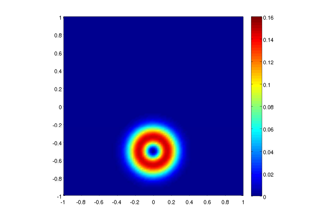
As shown in this figure, $SBP2$ and $SBP4$ schemes resolve the solution quite well. In fact, $SBP4$ is very accurate and keeps the hump intact throughout the rotation.

Grid size	$SBP2$	rate	$SBP4$	rate
40 $\times$ 40	$6.9\cdot 10^{1}$		$8.0\cdot 10^{0}$
80 $\times$ 80	$2.1\cdot 10^{1}$	1.7	$5.0\cdot 10^{-1}$	4.0
160 $\times$ 160	$5.5\cdot 10^{0}$	2.0	$4.5\cdot 10^{-2}$	3.5
320 $\times$ 320	$1.3\cdot 10^{0}$	2.0	$5.1\cdot 10^{-3}$	3.1
640 $\times$ 640	$3.3\cdot 10^{-1}$	2.0	$6.4\cdot 10^{-4}$	3.0

Table 1: Relative percentage errors in

l^{2}

for

|{\mathbf{B}}|

at time

t=2\pi

and rates of convergence for numerical experiment

1

with

SBP2

and

SBP4

schemes.

In Table 1, we present percentage relative errors in $l^{2}$ . The errors are computed at time $t=2\pi$ (one rotation) on a sequence of meshes for both the $SBP2$ and $SBP4$ schemes. The results show that the errors are quite low, particularly for $SBP4$ and the rate of convergence approaches the expected values of $2$ for $SBP2$ and $3$ for $SBP4$ . Furthermore, the order of accuracy is unaffected at these resolutions by using zero Dirichlet boundary data instead of the exact solution at the boundary.

In order to compare the SBP schemes of this paper with other existing schemes, we choose to compute the solutions for this problem with both the first- and the second-order divergence-preserving scheme of [23], which we label as the $TF$ and $TF2$ schemes. Furthermore, we compute the solutions using the first order stable upwind scheme designed in [6], labeled the $SUS$ scheme. The relative errors with each of these schemes are shown in Table 2.

Grid size	$SUS$	$TF$	$TF2$
40 $\times$ 40	$8.6\cdot 10^{1}$	$7.6\cdot 10^{1}$	$1.8\cdot 10^{1}$
80 $\times$ 80	$7.3\cdot 10^{1}$	$6.4\cdot 10^{1}$	$1.3\cdot 10^{1}$
160 $\times$ 160	$5.4\cdot 10^{1}$	$4.7\cdot 10^{1}$	$3.0\cdot 10^{0}$
320 $\times$ 320	$3.6\cdot 10^{1}$	$3.3\cdot 10^{1}$	$1.0\cdot 10^{0}$
640 $\times$ 640	$2.0\cdot 10^{1}$	$1.4\cdot 10^{1}$	$2.7\cdot 10^{-1}$

Table 2: Relative percentage errors in

l^{2}

for

|{\mathbf{B}}|

t=2\pi

and for numerical experiment

1

with the

SUS

TF

TF2

SBP2

and the

SBP4

schemes.

Results in Tables 1 and 2 show that the $TF$ and $SUS$ schemes lead to similar errors and these errors are considerably larger than the errors generated by the $TF2$ and $SBP2$ schemes, while the errors generated by the $SBP4$ scheme are much smaller again.

A fair comparison of the the five schemes SUS, TF, TF2, SBP2 and SBP4 requires information on the computational work with each scheme for the same error level. We observe from tables 1 and 2 that for a given relative error of approximately $20$ percent, the first-order SUS scheme requires a $640\times 640$ mesh, the TF scheme requires a $500\times 500$ mesh (based on extrapolation from table 2), whereas both the second-order schemes require meshes coarser than a $50\times 50$ mesh. The fourth-order scheme yields similar error levels on even coarser meshes. Thus, the second-order schemes require about $1\%$ of the total grid points to the first-order schemes to produce comparable errors. Even taking into account that the second order schemes use more operations for each grid point, this still makes the second order schemes at least $25-30$ times more efficient than the first order schemes. Similarly an error level of about one percent is attained with SBP2 on a $320\times 320$ mesh, with TF2 on a similar $320\times 320$ mesh and with SBP4 on a $50\times 50$ mesh. Thus the second order schemes need about $36$ times more grid points to produce errors similar to those of the fourth order schemes. Taking extra work for the fourth-order scheme per grid point into account, we still get that the fourth-order scheme is roughly $10$ times more efficient than the second-order schemes. These numbers are approximations but display a clear qualitative trend i.e., it is much more efficient to use high-order schemes for the induction equations.

As the solution (19) in this case is smooth, it is also a solution for the constrained form (3). Furthermore, the initial data is divergence free and so is the exact solution. We did not attempt to preserve any particular form of discrete divergence while designing the SBP schemes (15). A natural thing would be show that some form of discrete divergence produced by the schemes was bounded in $l^{2}$ . We were unable to obtain such a divergence bound for (15) in this paper. A related SBP-SAT scheme for the “conservative” symmetric form (5) with SBP operators for discretizing spatial derivatives coupled with a novel discretization of the source terms in (5) was shown to have bounded discrete divergence in a recent paper [14].

In the absence of a rigorous divergence bound, we proceed to examine how divergence errors generated by the SBP schemes behave and whether they have any impact on the quality of the discretization. We define the following discrete divergence,

\displaystyle\mathrm{div}_{P}(V)=(P_{x}^{-1}Q_{x}\otimes I_{y})V^{1}+(I_{x}\otimes P_{y}^{-1}Q_{y})V^{2}.

This corresponds to the standard centered discrete divergence operator at the corresponding order of accuracy. The divergence errors in $l^{2}$ and rates of convergence at time $t=2\pi$ for the $SBP2$ and $SBP4$ schemes on a sequence of meshes are presented in Table 3.

Grid size	$SBP2$	rate	$SBP4$	rate
20 $\times$ 20	$1.0\cdot 10^{0}$		$7.3\cdot 10^{-1}$
40 $\times$ 40	$8.0\cdot 10^{-1}$	0.4	$1.2\cdot 10^{-1}$	2.6
80 $\times$ 80	$2.7\cdot 10^{-1}$	1.6	$8.2\cdot 10^{-3}$	3.8
160 $\times$ 160	$7.0\cdot 10^{-2}$	2.0	$1.0\cdot 10^{-3}$	3.0
320 $\times$ 320	$2.5\cdot 10^{-2}$	1.5	$1.7\cdot 10^{-4}$	2.6

Table 3: Numerical Experiment

1

: Divergence (errors) in

l^{2}

and rates of convergence at time

t=2\pi

for both the

SBP2

and

SBP4

schemes.

From Table 3, we conclude that although the initial divergence is zero, the discrete divergence computed with both the $SBP2$ and $SBP4$ schemes is not zero. However, the divergence errors are very small even on fairly coarse meshes and converge to zero at a rate of $1.5$ and $2.5$ for $SBP2$ and $SBP4$ schemes respectively. A simple truncation error analysis suggests that these rates for the $SBP2$ and $SBP4$ schemes are optimal. The quality of the approximations is good and the rates of convergence do not seem to suffer from not preserving any form of discrete divergence.

In order to compare with existing schemes, we compare the divergence errors generated by the $SUS$ , $TF$ and the $TF2$ schemes with the $SBP2$ and the $SBP4$ schemes in table 4.

Grid size	$SUS$	$TF$	$TF2$
40 $\times$ 40	$1.1\cdot 10^{-1}$	$2.7\cdot 10^{-2}$	$1.2\cdot 10^{-2}$
80 $\times$ 80	$1.3\cdot 10^{-1}$	$1.7\cdot 10^{-2}$	$4.0\cdot 10^{-3}$
160 $\times$ 160	$1.4\cdot 10^{-1}$	$1.4\cdot 10^{-2}$	$2.4\cdot 10^{-3}$
320 $\times$ 320	$1.1\cdot 10^{-1}$	$1.2\cdot 10^{-2}$	$9.7\cdot 10^{-4}$

Table 4: Numerical Experiment

1

: The discrete divergence

\mathrm{div}_{P}

l^{2}

t=2\pi

for the

SUS

TF

and

TF2

schemes.

From Table 4, we can draw the following conclusions about divergence errors. The $SUS$ scheme is not tailored to preserve any form of discrete divergence. The divergence errors generated by this scheme seems to be low on coarse meshes. The $TF$ and $TF2$ schemes are designed to preserve a special form of discrete divergence which is different from the standard central form. Nevertheless, the analysis presented in [23] suggested that the errors in the standard divergence operator will also be quite low. This is indeed the case. On the coarser meshes, the divergence is much larger for the $SBP2$ scheme than the $TF$ schemes, but from Table 2 we see that the errors in the solution are similar.

Furthermore, the divergence errors converge quickly for the $SBP4$ scheme, as well as as the for the $TF2$ scheme. The above results indicate that controlling some form of discrete divergence is not necessary to approximate solutions of the magnetic induction equations in a stable and accurate manner.

Next, we consider long time integration. The energy estimate (17) suggests that the energy of the approximate solutions can grow exponentially in time. In order to test this we computed approximate solutions with the $SBP2$ , $SBP4$ and the $TF2$ schemes till time $t=100\pi$ , i.e., for fifty full rotations on a $100\times 100$ mesh. The numerical results in are presented in Figure 2 and Table 5.

$2\pi t$	$SBP2$	$SBP4$	$TF2$
$t=1$	$2.1\cdot 10^{1}$	$5.1\cdot 10^{-1}$	$8.8\cdot 10^{0}$
$t=5$	$7.7\cdot 10^{1}$	$2.7\cdot 10^{0}$	$3.2\cdot 10^{1}$
$t=10$	$1.0\cdot 10^{2}$	$4.7\cdot 10^{0}$	$5.0\cdot 10^{1}$
$t=15$	$1.1\cdot 10^{2}$	$6.6\cdot 10^{0}$	$6.3\cdot 10^{1}$
$t=20$	$1.2\cdot 10^{2}$	$8.7\cdot 10^{0}$	$7.2\cdot 10^{1}$
$t=30$	$1.2\cdot 10^{2}$	$1.9\cdot 10^{1}$	$8.4\cdot 10^{1}$
$t=40$	$1.3\cdot 10^{2}$	$3.1\cdot 10^{1}$	$9.2\cdot 10^{1}$
$t=50$	$1.4\cdot 10^{2}$	$4.3\cdot 10^{1}$	$1.0\cdot 10^{2}$

Table 5: Relative percentage

l^{2}

errors in

|{\mathbf{B}}|

with

SBP2

SBP4

and

TF2

for numerical experiment

1

These computations were performed on a fixed $100\times 100$ mesh. In Figure 2, we compare the $SBP2$ and $SBP4$ schemes after five and fifty rotations respectively. We see that after 5 rotations, $SBP2$ gives a “hump” which is somewhat smeared and with a pronounced asymmetry. On the other hand, the hump produced by the $SBP4$ scheme is much more accurate. As shown in Table 5, the absolute errors with the $SBP4$ scheme are much lower than the errors due to the second-order schemes $SBP2$ and $TF2$ . In fact, the errors with $SBP2$ after just five rotations are about three times the error with $SBP4$ after fifty rotations. This experiment makes a strong case for using high-order schemes for problems requiring long time integration.

Numerical Experiment $2$ : In the previous numerical experiment, the hump was confined to the interior of the domain during the rotation. Hence, the choice of zero Dirichlet data at the boundary was reasonable and led to stable and accurate approximations. In order to illustrate the effect of the boundary better, we choose the computational domain $[0,1]\times[0,1]$ and use the same velocity field and initial data as in the previous experiment. Now, the hump “exits” the domain at one part of the boundary (including a corner) and will re-enter the domain from another part of the boundary. The choice of boundary discretization becomes crucial in this case.

We select the exact solution (19) restricted to the boundary as the Dirichlet boundary data in (15).

In Figure 3, the approximate solutions computed with both $SBP2$ and $SBP4$ on a $100\times 100$ mesh are plotted at time $t=\pi/2$ (quarter rotation) and time $t=2\pi$ (full rotation). As shown in this figure, both schemes perform very well. The hump at both the exit as well as the re-entry is clearly resolved with no noticeable numerical artefacts or reflections.

Grid size	$SBP2$	rate	$SBP4$	rate
10 $\times$ 10	$2.5\cdot 10^{1}$		$1.1\cdot 10^{1}$
20 $\times$ 20	$5.8\cdot 10^{0}$	2.1	$1.5\cdot 10^{0}$	2.9
40 $\times$ 40	$1.3\cdot 10^{0}$	2.0	$1.6\cdot 10^{-1}$	3.3
80 $\times$ 80	$3.0\cdot 10^{-1}$	2.0	$1.6\cdot 10^{-2}$	3.2
160 $\times$ 160	$7.4\cdot 10^{-2}$	2.0	$1.9\cdot 10^{-3}$	3.1

Table 6: Numerical experiment

2

: Relative percentage errors for

|{\mathbf{B}}|

l^{2}

and rates of convergence for both

SBP2

and

SBP4

Grid size	$SBP2$	rate	$SBP4$	rate
10 $\times$ 10	$6.4\cdot 10^{-1}$		$9.7\cdot 10^{-2}$
20 $\times$ 20	$3.9\cdot 10^{-1}$	0.7	$2.4\cdot 10^{-2}$	2.0
40 $\times$ 40	$9.1\cdot 10^{-2}$	2.2	$1.9\cdot 10^{-3}$	3.6
80 $\times$ 80	$2.6\cdot 10^{-2}$	1.8	$3.0\cdot 10^{-4}$	2.7
160 $\times$ 160	$8.9\cdot 10^{-3}$	1.6	$5.1\cdot 10^{-5}$	2.5

Table 7: Numerical experiment

2

: Divergence (errors) in

l^{2}

and rates of convergence for both

SBP2

and

SBP4

at time

t=2\pi

As shown in Table 6, the errors are low after one full rotation for both the $SBP2$ and $SBP4$ schemes. In fact, the size of relative errors is lower than in the previous numerical experiment. As expected, the rates of convergence tend to $2$ and $3$ for $SBP2$ and $SBP4$ respectively. In Table 7 the divergence errors and their convergence rates are listed. They are small and the convergences approach the expected values $1.5$ and $2.5$ .

On the other hand, when we tried to compute this example with the divergence preserving $TF$ and $TF2$ schemes, the solution blew up on account of boundary instabilities.

Numerical Experiment 3: (Discontinuous solutions.) As remarked earlier, the magnetic induction equations (7) are a sub-model in the nonlinear MHD equations. As a consequence, one must solve the induction equation with both discontinuous velocity fields and initial data. It is therefore interesting to see how well the SBP-SAT schemes handle discontinuous velocity fields and initial data.

The SBP operators use centered finite differences in the interior. It is well known that using central differences leads to oscillations around discontinuities. Therefore the SBP schemes cannot be used directly in this regime, see [12] for details. To calculate solutions with discontinuities, one adds a small amount of explicit numerical diffusion that retain the accuracy of the first derivative SBP approximations as well as maintain the energy stability of the SBP scheme. We will use these operators together with the $SBP2$ and $SBP4$ schemes in order to compute discontinuous solutions of the magnetic induction equations.

The second-order (fourth-order) SBP operator for the first derivative with a second-order (fourth-order) numerical diffusion operator gives an approximation which is formally second-order (fourth-order) accurate in the interior of the computational domain. It turns out that a different scaling (dividing by the mesh size) of the numerical diffusion operator leads to a first order (third-order) “upwind” scheme. We will test all these numerical diffusion operators a numerical experiment first described in [6].

The computational domain is $[0,1]\times[0,1]$ . Consider the constant velocity field, ${\mathbf{u}}=(1,2)^{T}$ and the discontinuous initial data,

B^{1}_{0}(x,y)=B^{2}_{0}(x,y)=\begin{cases}2&\text{if $x>y$},\\ 0&\text{otherwise.}\end{cases}

In this case, the exact solution (see [6]) of (7) reads

{\mathbf{B}}(x,y,t)={\mathbf{B}}_{0}(x-t,y-2t).

The initial discontinuity simply moves along the diagonal of the domain. We use the exact solution restricted to the boundary as the Dirichlet boundary data. Tests with generic $SBP$ - $SAT$ schemes, (15), showed that the approximate solutions were very oscillatory, and we damp these oscillations by adding numerical diffusion.

We test the $SBP2$ ( $SBP4$ ) scheme with the standard second-order (fourth-order) numerical diffusion operator as well as the scaled numerical diffusion operator to obtain the first-order (third-order) $SBP1$ and $SBP3$ schemes. The results on a $100\times 100$ mesh at time $t=0.5$ are plotted in Figure 4.

A plot at this time is of interest as some part of the solution has interacted with the boundary and exited the domain, whereas most of the front is still inside the domain. From Figure 4, we see that the boundary discretization works well in all cases and does not lead to any significant oscillations in the domain. The $SBP1$ scheme is the most dissipative with significant smearing at the discontinuity. However, this scheme also has no over/under shoots or oscillations and the solution is $TVD$ . The $SBP2$ scheme with second-order numerical diffusion operator is oscillatory near the discontinuity with dispersive waves on both sides of it. The smearing is considerably less than that of the $SBP1$ scheme. The $SBP4$ scheme with standard fourth-order numerical diffusion is even more oscillatory and leads to a larger overshoot. The $SBP3$ scheme damps these oscillations somewhat and still keeps the sharpness at the discontinuity making it an acceptable alternative.

5 Conclusion

We have considered the magnetic induction equations that arise as a submodel in the MHD equations of plasma physics. Various forms of these equations were presented including the symmetric forms that are well-posed with general initial data and Dirichlet boundary conditions.

Standard numerical methods of the finite difference/finite volume type have dealt with discretizations of the constrained form (3) and attempted to preserve some form of the divergence constraint.

We describe $SBP$ - $SAT$ based finite difference schemes for the initial- boundary value problem corresponding to the magnetic induction equations. These schemes were based on the non-conservative symmetric form (4) and use $SBP$ finite difference operators to approximate spatial derivatives and a $SAT$ technique for implementing boundary conditions. The resulting schemes were energy stable and higher order accurate.

These schemes were tested on a series of numerical experiments, which illustrated their stability and high-order of accuracy. Interesting solution features were resolved very well. The fourth-order scheme was found to be well suited for long time integration problems. Despite the fact that the schemes were not preserving any particular form of discrete divergence as well as the lack of a rigorous discrete divergence bound, the divergence errors generated by the schemes were quite low and converged to zero at the expected rates when the mesh was refined. The schemes were compared with two existing lower order schemes and one divergence preserving second order scheme. Despite lacking any divergence bounds, the $SBP$ schemes performed at least as well as the schemes with a divergence bound.

The numerical experiments indicate that the $SBP$ - $SAT$ framework is effective in approximating solutions of the magnetic induction equations to a high order of accuracy. In the future we plan to extend these schemes to magnetic induction equations with resistivity.

References

(1) D.S. Balsara and D. Spicer. A staggered mesh algorithm using high order Godunov fluxes to ensure solenoidal magnetic fields in magnetohydrodynamic simulations. J. Comp. Phys., 149(2):270-292, 1999.
(2) N. Besse and D. Kröner. Convergence of the locally divergence free discontinuous Galerkin methods for induction equations for the 2D-MHD system. M2AN Math. Model. Num. Anal 39(6):1177-1202, 2005.
(3) J.U. Brackbill and D.C. Barnes. The effect of nonzero $\mathrm{div}B$ on the numerical solution of the magnetohydrodynamic equations. J. Comp. Phys., 35:426-430, 1980.
(4) W. Dai and P.R. Woodward. A simple finite difference scheme for multi-dimensional magnetohydrodynamic equations. J. Comp. Phys., 142(2):331-369, 1998.
(5) C. Evans and J.F. Hawley. Simulation of magnetohydrodynamic flow: a constrained transport method. Astrophys. J., 332:659, 1998.
(6) F. Fuchs, K.H. Karlsen, S. Mishra and N.H. Risebro. Stable upwind schemes for the Magnetic Induction equation. Preprint, Submitted.
(7) F. Fuchs, S. Mishra and N.H. Risebro. Splitting based finite volume schemes for ideal MHD equations. in press Jl. Comput. Phys.,
(8) S.K. Godunov. The symmetric form of magnetohydrodynamics equation. Num. Meth. Mech. Cont. Media, 1:26-34, 1972.
(9) B. Gustafsson, H.-O. Kreiss, and J. Oliger. Time dependent problems and difference methods. John Wiley & Sons, Inc., 1995.
(10) H.O. Kreiss and J. Lorenz. Initial-Boundary value problems and the Navier–Stokes equations. Academic Press, Boston, 1989.
(11) R.J. LeVeque. Finite volume methods for hyperbolic problems. Cambridge university press, Cambridge, 2002.
(12) K. Mattsson, M. Svärd and J. Nordström. Stable and Accurate Artificial Dissipation. Journal of Scientific Computing, Vol.21,No.1, August 2004.
(13) K. Mattsson and J. Nordström. Summation by parts operators for finite difference approximations of second derivative. Journal of Computational Physics, 199(2004), 503-540.
(14) S. Mishra and M. Svärd. On stability of numerical schemes via frozen coefficients and magnetic induction equations. Preprint, Submitted.
(15) J. Nordström. Error Bounded Schemes for Time-dependent Hyperbolic Problems SIAM J. Sci. Comput., 30(2007), 46-59.
(16) J. Nordström and M. H. Carpenter High-Order Finite Difference Methods, Multidimensional Linear Problems, and Curvilinear Coordinates J. Comput. Phys, 173(2001), 149-174.
(17) K.G. Powell. An approximate Riemann solver for magneto-hydro dynamics (that works in more than one space dimension). Technical report, 94 -24, ICASE, Langley, VA, 1994.
(18) K.G. Powell, P.L. Roe. T.J. Linde, T.I. Gombosi and D.L. De Zeeuw, A solution adaptive upwind scheme for ideal MHD. J. Comp. Phys, 154(2), 284 - 309, 1999
(19) J. Rauch. Partial Differential Equations, Springer, 1991.
(20) D.S. Ryu, F. Miniati, T.W. Jones and A. Frank. A divergence free upwind code for multidimensional magnetohydrodynamic flows. Astrophys. J., 509(1):244-255, 1998.
(21) M. Svärd On coordinate transformations for summation-by-parts operators J. Sci. Comput. 20(2004), 29-42.
(22) M. Svärd and J. Nordström. On the order of accuracy for difference approximations of initial-boundary value problems. Journal of Computational Physics, 218(2006), 333-352.
(23) M. Torrilhon and M. Fey. Constraint-preserving upwind methods for multidimensional advection equations. SIAM. J. Num. Anal., 42(4):1694-1728, 2004.
(24) G. Toth. The $\mathrm{div}B=0$ constraint in shock capturing magnetohydrodynamics codes. J. Comp. Phys.,161:605-652, 2000.