跳到论文正文
W Papers独立论文阅读器 arXiv:1102.0331 论文正文 计算阅读时间 · 0%
引用这篇论文根据当前论文元数据生成,正式投稿前建议核对。


License: arXiv.org perpetual non-exclusive license
arXiv:1102.0331v2 [hep-ph] 18 Jun 2011

Minimal Prescription Corrected Spectra
in Heavy Quark Decays

L. Di Giustino a,    G. Ricciardi b,    L. Trentadue c

aSLAC National Accelerator Laboratory,
Stanford University, Stanford, CA 94309, USA
bDipartimento di Fisica, Università di Napoli ”Federico II”
and
INFN Sezione di Napoli, Napoli, Italy
cDipartimento di Fisica, Università di Parma,
and
INFN, Gruppo Collegato di Parma, Parma, Italy

The Minimal Prescription procedure is applied to tame the Landau pole singularities of resummed formulae for heavy quark decays. Effects of the final quark mass are taken into account. Explicit expressions are obtained for the t→bt\rightarrow b and b→cb\rightarrow c transitions for both the frozen coupling approximation and in the QCD running coupling case.

1 Introduction

A common feature to many processes in QCD is the presence, in the perturbative expansion, of large double (Sudakov-like) logarithms at the threshold. Resummation of large infrared logarithms in form factors and shape variables is essential in order to predict accurate cross sections in many phenomenologically relevant processes (see, f.i. [1, 2, 5, 3, 4]). In semi-leptonic heavy quark decays qi→qf​l​νq_{i}\rightarrow q_{f}\,l\,\nu, threshold regions are characterized by the presence of two different scales mX≪EXm_{X}\ll E_{X}, where mXm_{X} and EXE_{X} are the final hadron invariant mass and energy, respectively, originated by the final quark qfq_{f}. The perturbative expansion is spoiled by logarithms of the ratio of the two scales. Those need, therefore, to be resummed.

Such logarithms are organized as a series of the form [6, 7]:

∑n=1∞∑k=12​ncn​k​αsn​(Q)​logk​Q2mX2=c12​αs​(Q)​log2​Q2mX2+c11​αs​(Q)​log⁡Q2mX2+\displaystyle\sum_{n=1}^{\infty}\sum_{k=1}^{2n}c_{nk}\,\alpha_{s}^{n}(Q)\,\log^{k}\frac{Q^{2}}{m_{X}^{2}}=\;\;\;c_{12}\,\alpha_{s}(Q)\,\log^{2}\frac{Q^{2}}{m_{X}^{2}}\,+\,c_{11}\,\alpha_{s}(Q)\,\log\frac{Q^{2}}{m_{X}^{2}}\,+ (1)
+\displaystyle+ c24​αs2​(Q)​log4​Q2mX2+c23​αs2​(Q)​log3​Q2mX2+⋯,\displaystyle\,c_{24}\,\alpha_{s}^{2}(Q)\,\log^{4}\frac{Q^{2}}{m_{X}^{2}}\,+\,c_{23}\,\alpha_{s}^{2}(Q)\,\log^{3}\frac{Q^{2}}{m_{X}^{2}}\,+\,\cdots,

where αs\alpha_{s} is the QCD coupling constant and QQ is the hard scale Q=2​EXQ=2\,E_{X}. The leading term is the double logarithm αs​(Q)​log2​Q2mX2\alpha_{s}(Q)\,\log^{2}\frac{Q^{2}}{m_{X}^{2}}. A similar double logarithmic structure is present in many other processes like deep inelastic scattering (DIS), heavy quark fragmentation, Drell-Yan annihilation, Higgs production, and so on, the argument of the logarithms differing per observable and per process.

A universal resummation formula valid at all perturbative orders for a decay of a heavy quark qiq_{i} into a massive quark qfq_{f} plus a non-hadronic state, with a final state jet-like structure, has been recently obtained [8].

In QCD resummed formulas, the running coupling is integrated over all gluon radiative momenta from the hard scale down to zero, hitting the Landau pole. A prescription has to be assigned to give a meaning to the formal resummed expressions.

One possible solution is the use of an additional prescription for the contour integration in NN-space, in the inverse Mellin transform from NN-space to xx-space, the so-called minimal-prescription (MP) [9]. This prescription provides a formula which is the asymptotic limit of the expansion, furthermore it is renormalon free and the truncation of the series at the minimum term originates an exponentially suppressed difference between the truncated expansion and the full MP formula.

The aim of this work is to analyze the perturbative resummed distributions in the parton subprocess for both massless and massive final heavy quarks and to explore the feasibility of the MP regularization scheme.

We apply the resummation formulas to the case of t→bt\rightarrow b and b→cb\rightarrow c, as a working example to implement this regulation method. In literature, the b→cb\rightarrow c inclusive semileptonic decays are widely discussed, also in the contest of effective theories, in order to improve comparison with the newest data (for a review see f.i [10] and refs within). The t→bt\rightarrow b case has been discussed in QCD resummed formulas [11], with different dynamical variables.

The assessment of a perturbative reliable and singularity safe form factor is the first step towards a sound phenomenological approach and it is also needed for comparison with QCD based effective theories like, for example, SCET.

The papers is organized as follows: in section 2 we recall the resumming formulas for the final massless and massive quark in the Mellin space, and recast them in a more transparent notation; in section 3 we move to the physical space and analyze the feasibility of the MP for the massive case. In section 4 we study the frozen coupling approximation, while final plots with the QCD running coupling and conclusions are presented in sections 5 and 6.

2 Threshold resummed Jet Distribution in Mellin space

2.1 Massless final quark

Before considering the case of a massive final case, let us recall the expressions and the variables for the resummed jet distributions in the massless final state [5, 13, 14, 12, 15].

Let us consider the decay driven at a partonic level by an heavy quark decaying into an approximately massless final quark, plus non-hadronic states, as, for instance, the decay B→Xu​l​νB\rightarrow X_{u}l\nu or the radiative decay B→Xs​γB\rightarrow X_{s}\gamma. Threshold resummation is typically performed in Mellin space; the threshold limit corresponds to N→∞N\rightarrow\infty and threshold logarithms αsn​logm​N\alpha_{s}^{n}\log^{m}N can be factorized into a form factor JNJ_{N}, which has the exponential form:

JN​(Q2)=efN​(Q2),J_{N}(Q^{2})\,=\,e^{\,f_{N}\left(Q^{2}\right)}, (2)

JN​(Q2)J_{N}(Q^{2}) is the massless jet distribution, that gives the probability that a massless parton produced in a hard process with a hard scale QQ fragments into a hadronic jet of mass mXm_{X}

mX2=(1−x)​Q2m^{2}_{X}=(1-x)Q^{2} (3)

The Mellin or N−N- transform is defined as

JN​(Q2)≡∫01d​x​xN−1​J​(x,Q2)J_{N}(Q^{2})\equiv\int_{0}^{1}dx\,x^{N-1}J(x;Q^{2}) (4)

In the limit αs→0\alpha_{s}\rightarrow 0, the mass distribution reduces to a spike corresponding to the (zero) parton mass. In the limit x→1x\rightarrow 1 we drift away from the perturbative regime. If x=1x=1, the truncated perturbative expansion becomes unreliable. It is possible, however, to be able to use a perturbative resummed expression at all orders in the Mellin space which reads [5, 13, 14, 12, 15]:

JN​(Q2)\displaystyle J_{N}(Q^{2}) =\displaystyle= exp∫01d​x1−x[xN−1−1]{∫Q2​(1−x)2Q2​(1−x)d​k⟂2k⟂2A[αs(k⟂2)]+B[αs(Q2(1−x))]+\displaystyle\exp\int_{0}^{1}\frac{dx}{1-x}\left[x^{N-1}-1\right]\Bigg\{\int_{Q^{2}(1-x)^{2}}^{Q^{2}(1-x)}\frac{dk_{\perp}^{2}}{k_{\perp}^{2}}A\left[\alpha_{s}\left(k_{\perp}^{2}\right)\right]\,+\,B\left[\alpha_{s}\left(Q^{2}(1-x)\right)\right]\,+\, (5)
+D[αs(Q2(1−x)2)]}\displaystyle+D\left[\alpha_{s}\left(Q^{2}(1-x)^{2}\right)\right]\Bigg\}

The functions A⁡(αs)A\left(\alpha_{s}\right), B⁡(αs)B\left(\alpha_{s}\right) and D⁡(αs)D\left(\alpha_{s}\right) have a perturbative expansion:

A⁡(αs)=A1​αs+A2​αs2+⋯,B⁡(αs)=B1​αs+B2​αs2+⋯,D⁡(αs)=D1​αs+D2​αs2+⋯.A\left(\alpha_{s}\right)=A_{1}\alpha_{s}+A_{2}\alpha_{s}^{2}+\cdots,\quad B\left(\alpha_{s}\right)=B_{1}\alpha_{s}+B_{2}\alpha_{s}^{2}+\cdots,\quad D\left(\alpha_{s}\right)=D_{1}\alpha_{s}+D_{2}\alpha_{s}^{2}+\cdots. (6)

The known values of the coefficients AiA_{i}, BiB_{i} and DiD_{i} are given in [14, 16, 17].

A⁡(αs)A\left(\alpha_{s}\right) describes the emission of partons which are both soft and collinear, B⁡(αs)B\left(\alpha_{s}\right) describes hard and collinear partons while D⁡(αs)D\left(\alpha_{s}\right) partons which are emitted soft at large angles. A⁡(αs)A(\alpha_{s}) and B⁡(αs)B(\alpha_{s}) are related to small-angle emission only. They, therefore, represent intra-jet properties[17, 16], while the function D⁡(αs)D(\alpha_{s}), being related to soft emissions at large angles, is a process-dependent inter-jet quantity.

While the validity of the resummed formula goes beyond our case of semi-leptonic heavy quark decays, holding for accounting of threshold logarithms in several other processes, the specific structure of (5) can vary, depending on the specific process and on the particular observable under exam. For instance, there are corresponding results for the DIS structure functions F1,2,3​(x,Q2)F_{1,2,3}(x,Q^{2}), where Q2Q^{2} represents the resolution scale, or for the Drell-Yan cross section d​σ/d​Q2d\sigma/dQ^{2}, where Q2Q^{2} stands for the invariant mass squared of the lepton pair [13, 18].

In order to illustrate how to interpret the universality of formula (5), let us consider the order αs\alpha_{s} decay t→b​W​gt\rightarrow\,b\,W\,g (where WW and gg are a real W boson and a gluon, respectively) and examine the distribution in the energy of the final bb-quark, that is in the variable xb=2​Eb/mtx_{b}=2E_{b}/m_{t}. Once considering the distribution in xbx_{b}, rather than in xx as in the present paper (see definition (3)), we are dealing with a different observable–and therefore a different kinematical parametrization of the threshold region. Now the threshold region is reached when xb→1x_{b}\rightarrow 1, a limiting point where there is no gluon emission to change the light quark energy. We expect only the emission of soft gluons and we do not need any B⁡(αs)B(\alpha_{s}) contribution in (5), since this function contains collinear radiation associated with the light quark. Formula (5) still holds, but without the B⁡(αs)B(\alpha_{s}) term[11]. In the present work, collinear gluons described by B⁡(αs)B(\alpha_{s}) are allowed, since the energy change of the light quark, still in the jet after the gluon emission, does not affect the distributions in xx, related to the invariant mass of the jet.

The exponent of Eq. (2) can be expanded in a function series of the form [13]:

fN​(Q2)=log⁡JN​(Q2)=L​g1​(λ)+∑n=0∞αsn​gn+2​(λ)=L​g1​(λ)+g2​(λ)+αs​g3​(λ)+⋯,f_{N}(Q^{2})=\log J_{N}(Q^{2})=L\,g_{1}\left(\lambda\right)+\sum_{n=0}^{\infty}\alpha_{s}^{n}\,g_{n+2}\left(\lambda\right)=L\,g_{1}\left(\lambda\right)+\,g_{2}\left(\lambda\right)+\alpha_{s}\,g_{3}\left(\lambda\right)+\cdots, (7)

where

λ=β0​αs​(Q2)​L,L=log⁡N\lambda~=~\beta_{0}~\alpha_{s}(Q^{2})~L,~~~~~~~L~=~\log N (8)

and β0=(11/3​NC−2/3​nF)/(4​π)\beta_{0}=(11/3\;N_{C}-2/3\;n_{F})/(4\pi).

The first exponential term L​g1​(λ)=L​∑n=1∞g1,n​λnL\,g_{1}\left(\lambda\right)=L\,\sum_{n=1}^{\infty}g_{1,n}\lambda^{n} resums the leading logarithms (LL); by adding the term g2​(λ)=∑n=1∞g2,n​λng_{2}\left(\lambda\right)=\sum_{n=1}^{\infty}g_{2,n}\lambda^{n}, also next-to-leading order terms (NLL) are taken into account and resummed, and so on.

The functions gi​(λ)g_{i}\left(\lambda\right) have a power-series expansion:

gi​(λ)=∑n=1∞gi,n​λn.g_{i}\left(\lambda\right)=\sum_{n=1}^{\infty}g_{i,n}\lambda^{n}. (9)

They are all homogeneous functions: gi​(0)=0g_{i}(0)=0. This property insures the normalization of the form factor JN=1=1J_{N=1}=1. The functions g1g_{1} and g2g_{2} become singular, signaling non-perturbative effects, at λ=1/2\lambda=1/2, that is at N=exp⁡[1/2​β0​αs​(μ2)]≈μ2/Λ2N=\exp[1/2\beta_{0}\alpha_{s}(\mu^{2})]\approx\mu^{2}/\Lambda^{2}. Explicit expressions are given in [19, 20].

The leading logarithmic term in Eq. (5) is

JN≃exp⁡[L​g1​(λ)]≃exp⁡[−A12​αs​L2]=exp⁡[−CF2​π​αs​log2​N]J_{N}\simeq\exp\left[L\,g_{1}\left(\lambda\right)\right]\simeq\exp\left[-\frac{A_{1}}{2}\alpha_{s}L^{2}\right]=\exp\left[-\frac{C_{F}}{2\pi}\alpha_{s}\log^{2}N\right] (10)

Function series like Eq. (7) appear in other processes as well as, for instance, DIS and Drell-Yan with the same towers of threshold logarithms. Additional terms, however, due to soft-gluon radiation collinear to the light initial-state parton, in the DIS case, and to two light initial-state partons, in the Drell-Yan case, do slightly modify the form of g1g_{1}, giving, for the leading term of the resummed quark coefficient functions CD​I​SNC^{N}_{DIS} and CD​YNC^{N}_{DY}[18] respectively :

CD​I​SN∝exp⁡[L​g1D​I​S​(λ)]≃exp⁡[CF2​π​αs​log2​N]CD​YN∝exp⁡[L​g1D​Y​(λ)]≃exp⁡[2​CFπ​αs​log2​N]C^{N}_{DIS}\propto\exp\left[L\,g_{1}^{DIS}\left(\lambda\right)\right]\simeq\exp\left[\frac{C_{F}}{2\pi}\alpha_{s}\log^{2}N\right]\qquad C^{N}_{DY}\propto\exp\left[L\,g_{1}^{DY}\left(\lambda\right)\right]\simeq\exp\left[2\frac{C_{F}}{\pi}\,\alpha_{s}\log^{2}N\right] (11)

We plot in fig. 1 the form factor in the massless case, for the t→bt\rightarrow b and the b→b\rightarrow decays, in order to show the different slopes in the two cases, that will be maintained in the massive case, affecting the regularization procedure. We have set the scale μ\mu in gig_{i} equal to Q2Q^{2}. The continuous and dashed lines represent the NLL and NNLL contributions respectively. The strong dependence on αs\alpha_{s} values is shown: light and thick lines are referred to different values of αs\alpha_{s}. The NNLL curve stands below the NLL one, due to the inclusion of g3g_{3}, that is a negative decreasing function within the considered range. We also observe a relatively strong dependence on αs\alpha_{s}. As said before, the effects of the Landau pole start appearing at λ=1/2\lambda=1/2, that is towards N∼106N\sim 10^{6} for the case of the top decay, and for N∼102N\sim 10^{2} for the case of bottom decay; there, the Mellin form factor starts to oscillate and the expressions are no longer predictive.

Refer to caption
Refer to caption
Figure 1: Form factor in N space for massless final quark. Left figure: the t→bt\rightarrow b case: αs=0.11\alpha_{s}=0.11 (light lines), αs=0.12\alpha_{s}=0.12 (thick lines). Right figure: the b→cb\rightarrow c case, αs=0.20\alpha_{s}=0.20 (light lines), αs=0.22\alpha_{s}=0.22 (thick lines). In both figures the continuous lines represent NLL contributions, the dashed lines NNLL contributions.

2.2 Mass-corrected Jet Distribution

Let us briefly summarize the results obtained for the case of a massive final quark qfq_{f} [8]. The more massive is the radiating qfq_{f}, the less radiation has to be emitted in the decay; as a consequence, the typical Sudakov effect, namely the suppression of non-radiative channels and the broadening of sharp structures, are expected to be less pronounced for the massive channels. In principle one has single-logarithmic corrections, which are not strong enough to shift the peak of tree-level distributions.

In Ref.[8] it was demonstrated at NNL order (and conjectured to be also valid at accuracy beyond NNL) that the massive jet function can be factorized in momentum space, as:

JN​(Q2,r)=JN​(Q2)​δN​(Q2,r)J_{N}(Q^{2};\,r)\,=\,J_{N}(Q^{2})~\delta_{N}(Q^{2};\,r) (12)

JN​(Q2)J_{N}(Q^{2}) is the massless jet distribution and δN​(Q2,r)\delta_{N}(Q^{2};\,r) is the mass-correction factor which reads:

δN​(Q2,r)\displaystyle\delta_{N}(Q^{2};\,r) =\displaystyle= exp∫01dxxr⁡(N−1)−11−x{−∫m2​(1−x)2m2​(1−x)d​k⟂2k⟂2A[αs(k⟂2)]−B[αs(m2(1−x))]+\displaystyle\exp\int_{0}^{1}dx\frac{x^{\,r\,(N-1)}-1}{1-x}\Bigg\{-\int_{m^{2}(1-x)^{2}}^{m^{2}(1-x)}\frac{dk_{\perp}^{2}}{k_{\perp}^{2}}A\left[\alpha_{s}\left(k_{\perp}^{2}\right)\right]-B\left[\alpha_{s}\left(m^{2}(1-x)\right)\right]+ (13)
+D[αs(m2(1−x)2)]},\displaystyle\,+\,D\left[\alpha_{s}\left(m^{2}(1-x)^{2}\right)\right]\Bigg\},

xx and rr are defined as

y≡1−x≡mX2−m2Q2−m2r≡m2Q2≪ 1y\equiv 1-x\,\equiv\,\frac{m_{X}^{2}-m^{2}}{Q^{2}-m^{2}}\qquad\qquad r\,\equiv\,\frac{m^{2}}{Q^{2}}\,\ll\,1 (14)

where QQ is the hard scale of the process and mm is the mass of the emitting quark. We assume the quark mass to be much smaller than the hard scale, in order to have fast-moving charges and to preserve a jet structure. We indicate both the mass corrected and the massless jet functions with JNJ_{N}; they are distinguishable since the the massive one bears a dependence on rr.

Eq. (13) has a simple physical interpretation. The parameter N−1N-1 is multiplied by rr on the r.h.s. of Eq. (13), implying that mass effects become “visible” only for large

N≥1r≫ 1.N\,\geq\,\frac{1}{r}\,\gg\,1. (15)

In this case, there is enough resolution to “see” the quark mass, which tends to suppress the collinear effects, related to the AA and BB terms. At the same time, soft radiation not collinearly enhanced, described by the function DD and characteristic of massive partons, does appear. Let us also note that, since the jet mass is an infrared (i.e. soft and collinear) safe quantity, δN=1\delta_{N}=1 for r=0r=0. In the limit r→ 0r\,\to\,0, the well-known massless result is recovered.

The mass-correction factor has the same structure than the massless case [13]

δN​(Q2,r)=eFN​(Q2,r),\delta_{N}(Q^{2};\,r)\,=\,e^{F_{N}\left(Q^{2};r\right)}, (16)

where the exponent has a double expansion of the form:

FN​(Q2,r)=θ⁡(N−1/r)​∑n=1∞∑k=1n+1Fn​k​αsn​logk⁡(N​r),F_{N}\left(Q^{2};r\right)\,=\,\theta\left(N-1/r\right)\,\sum_{n=1}^{\infty}\sum_{k=1}^{n+1}F_{nk}\,\alpha_{s}^{n}\log^{k}(Nr), (17)

with Fn​kF_{nk} numerical coefficients. The exponent can be expanded in towers of logarithms as:

FN​(Q2,r)\displaystyle F_{N}\left(Q^{2};r\right) =\displaystyle= L​d1​(ρ)+∑n=0∞αsn​dn+2​(ρ)\displaystyle L\,d_{1}\left(\rho\right)\,+\,\sum_{n=0}^{\infty}\alpha_{s}^{n}\,d_{n+2}\left(\rho\right) (18)
=\displaystyle= L​d1​(ρ)+d2​(ρ)+αs​d3​(ρ)+αs2​d4​(ρ)+⋯,\displaystyle L\,d_{1}\left(\rho\right)\,+\,d_{2}\left(\rho\right)\,+\,\alpha_{s}\,d_{3}\left(\rho\right)\,+\,\alpha_{s}^{2}\,d_{4}\left(\rho\right)\,+\,\cdots,

where

ρ≡β0​αs​(μ2)​L,and​L=θ⁡(N−1/r)​log⁡(N​r).\rho\,\equiv\,\beta_{0}\alpha_{s}(\mu^{2})\,L,\,\,\mathrm{and}\,\,\,L=\,\,\theta\left(N-1/r\right)\,\log\left(N\,r\right). (19)

The scale μ=O⁡(m)\mu=O(m) is a renormalization scale of the order of the quark mass mm. The over-all factor θ⁡(N−1/r)\theta\left(N-1/r\right) comes from the step approximation of the moment kernel and avoids modifications for small NN of the massless behavior, in agreement with the physical intuition. Furthermore it ensures the correct massless behavior in the r→0r\rightarrow 0 limit. Analytic continuation to the complex NN-plane can be made by omitting such factor and fixing the correct interval in physical space.

By truncating the above series expansion, one obtains a fixed-logarithmic approximation to the form factor δN\delta_{N}. Functions di​(ρ)d_{i}(\rho), which represent the mass effects, can be obtained from the standard ones gi​(λ)g_{i}(\lambda) of the massless case [7] by means of the replacements:

A⁡(αs)→−A⁡(αs);B⁡(αs)→−B⁡(αs);D⁡(αs)→D⁡(αs);log⁡μ2Q2→log⁡μ2m2;λ→ρ.A(\alpha_{s})\,\to\,-\,A(\alpha_{s});~~B(\alpha_{s})\,\to\,-\,B(\alpha_{s});~~D(\alpha_{s})\,\to\,D(\alpha_{s});~~\log\frac{\mu^{2}}{Q^{2}}\,\to\,\log\frac{\mu^{2}}{m^{2}};~~\lambda\,\to\,\rho. (20)

It is worth observing that mass effects induce a similar structure to the massless one, involving changes of sign of the collinear functions AA and BB, with the rescaling Q→mQ\,\to\,m. The explicit expressions for the functions did_{i} are listed in [8].

Let us now examine the behaviour of the jet function as given by the equation (12). Throughout the paper we fix the hard scale of the process QQ to the mass of the decaying quark, that is to mtm_{t} in the case of top decays, and to mbm_{b} for b decays. The correction factor δN​(Q2,r)\delta_{N}(Q^{2};\,r) is a function increasing with NN; in order to produce JN​(Q2,r)J_{N}(Q^{2};\,r) it has to be multiplied by the massless form factor JN​(Q2)J_{N}(Q^{2}), at values of N>1/rN>1/r. In the case of the top quark decay, the increase is very slow; it starts at 1/r∼2​x​ 1031/r\sim 2\,\textrm{x}\,10^{3} and the distribution only doubles when NN reaches ∼6​x​ 104\sim 6\,\textrm{x}\,10^{4}, continuing slowly, until a fast increase before values of ∼2​x​ 10​mt2/Λ2∼106\sim 2\,\textrm{x}\,10\,\,m_{t}^{2}/\Lambda^{2}\sim 10^{6}, where it reaches the peak 11 1 Differences between the mass correction factor at NNLL and NLL order are that the NNLL corrected one peaks much faster and at an earlier point in NN; the increase, however, still occurs at the same order of magnitude and it does not introduce substantial changes on the distribution.. That implies, as expected, that mass addition does not modify substantially the massless distribution until very large values of NN. The left hand plot in fig. 1 practically coincides with JN​(Q2,r)J_{N}(Q^{2},r) defined in (12), at the same value of αs\alpha_{s}.

On the contrary, in the b→cb\rightarrow c case, the increase starts earlier (1/r∼2​x​ 101/r\sim 2\,\textrm{x}\,10) and it is much faster (it doubles one at N∼102N\sim 10^{2}), reaching the fast increase and the peak around N∼mb2/Λ2N\sim m_{b}^{2}/\Lambda^{2}; effects are much more sizable. NNLL corrected curves grow faster than the NLL curves, as shown in fig. 2.

Refer to caption
Figure 2: Form factor in N space for b→cb\to c at αs=0.219\alpha_{s}=0.219: the continuous and dashed lines represent NLL and NNLL contributions, respectively. Light and thick lines refer here to massive and massless final quark, respectively.

3 Threshold resummed Jet Distribution in physical space

Even if the NN-moment expressions of the jet function are physical quantities, their measurement, especially for large NN, is difficult. It is therefore convenient to perform the inverse Mellin transform back to momentum space. Given the Mellin transform JNJ_{N} defined as in (4), its inverse transform is

J⁡(x,Q2)=M−1​[JN;x]=12​π​i​∫C−i​∞C+i​∞d​N​x−N​JN​(Q2)J(x;Q^{2})=M^{-1}[J_{N};x]=\frac{1}{2\pi i}\int_{C-i\infty}^{C+i\infty}dN\,x^{-N}J_{N}(Q^{2}) (21)

The inverse transform of the product of two generic fNf_{N} and gNg_{N} is the convolution of the two inverse functions f⁡(x)f(x) and g⁡(x)g(x):

M−1​[fN​gN;x]=∫x1f⁡(xu)​g​(u)​d​uuM^{-1}[f_{N}\,g_{N};x]=\int_{x}^{1}f\left(\frac{x}{u}\right)g(u)\frac{du}{u} (22)

3.1 Massless final quark

There are two possible ways of obtaining the J⁡(x,Q2)J(x;Q^{2}) distribution from the inverse Mellin trasform. Each of them has its own peculiarities, since we are dealing with truncated expressions. We have used both in order to compare the results and increase their reliability.

One way is to use an analytical expression for the inverse Mellin transform (21). Indeed, the massless form factor JN​(Q2)J_{N}(Q^{2}) is

J⁡(x,Q2)=−x​dd​x​{θ⁡(1−x−ϵ)​Σ​(x,Q2)}atϵ→0,J(x;Q^{2})=-x\,\frac{d}{dx}\Big\{\theta\left(1-x-\epsilon\right)\,\Sigma\left(x;\,Q^{2}\right)\Big\}\qquad\qquad\textrm{at}\quad\epsilon\rightarrow 0, (23)

where Σ⁡(x,Q2)\Sigma(x;Q^{2}) is the inverse Mellin transform of JN/NJ_{N}/N.

The θ⁡(1−x)\theta(1-x) function ensures the unitary normalization of the distribution in the interval (0,1)(0,1) and it can be omitted in the massless case since the function is regular at the origin.

We have, at NNLL [19] that :

Σ⁡(x,Q2)\displaystyle\Sigma(x;Q^{2}) =\displaystyle= eF0​(l)Γ⁡(1−F1N​L)​[1+F1N2​L​ψ​(1−F1N​L)+12​F2​(l)​(ψ2​(1−F1N​L)−ψ′​(1−F1N​L))]\displaystyle\frac{e^{F_{0}(l)}}{\Gamma(1-F_{1}^{NL})}\left[1+{F_{1}^{N^{2}L}}\,\psi(1-{F_{1}^{NL}})+\frac{1}{2}\,F_{2}(l)\,\left(\psi^{2}(1-{F_{1}^{NL}})-\psi^{\prime}(1-{F_{1}^{NL}})\right)\right]
=\displaystyle= el​g1​(β0​αs​l)+g2​(β0​αs​l)+αs​g3​(β0​αs​l)Γ⁡(1−g1​(β0​αs​l)−β0​αs​l​g1′​(β0​αs​l))[1+β0αsg2′(β0αsl)ψ(1−g1(β0αsl)−β0αslg1′(β0αsl))\displaystyle\frac{e^{l\,g_{1}(\beta_{0}\alpha_{s}l)+g_{2}(\beta_{0}\alpha_{s}l)+\alpha_{s}\,g_{3}(\beta_{0}\alpha_{s}l)}}{\Gamma(1-g_{1}(\beta_{0}\alpha_{s}l)-\beta_{0}\alpha_{s}\,l\,g_{1}^{\prime}(\beta_{0}\alpha_{s}l))}\left[1+\beta_{0}\alpha_{s}\,g_{2}^{\prime}(\beta_{0}\alpha_{s}l)\,\psi(1-g_{1}(\beta_{0}\alpha_{s}l)-\beta_{0}\alpha_{s}\,l\,g_{1}^{\prime}(\beta_{0}\alpha_{s}l))\right.
+12F2(l)(ψ2(1−g1(β0αsl)−β0αslg1′(β0αsl))−ψ′(1−g1(β0αsl)−β0αslg1′(β0αsl)))]\displaystyle\left.+\frac{1}{2}\,F_{2}(l)\,\left(\psi^{2}(1-g_{1}(\beta_{0}\alpha_{s}l)-\beta_{0}\alpha_{s}\,l\,g_{1}^{\prime}(\beta_{0}\alpha_{s}l))-\psi^{\prime}(1-g_{1}(\beta_{0}\alpha_{s}l)-\beta_{0}\alpha_{s}\,l\,g_{1}^{\prime}(\beta_{0}\alpha_{s}l))\right)\right]

where

F0​(l)\displaystyle F_{0}(l) =\displaystyle= l​g1​(β0​αs​l)+g2​(β0​αs​l)+αs​g3​(β0​αs​l),\displaystyle l\,g_{1}(\beta_{0}\alpha_{s}l)+g_{2}(\beta_{0}\alpha_{s}l)+\alpha_{s}\,g_{3}(\beta_{0}\alpha_{s}l),
F1N​L​(l)\displaystyle F_{1}^{NL}(l) ≡\displaystyle\equiv g1​(β0​αs​l)+β0​αs​l​g1′​(β0​αs​l)\displaystyle g_{1}(\beta_{0}\alpha_{s}l)+\beta_{0}\alpha_{s}\,l\,g_{1}^{\prime}(\beta_{0}\alpha_{s}l)
F1N2​L​(l)\displaystyle F_{1}^{N^{2}L}(l) ≡\displaystyle\equiv β0​αs​g2′​(β0​αs​l).\displaystyle\beta_{0}\alpha_{s}\,g_{2}^{\prime}(\beta_{0}\alpha_{s}l).
F2​(l)\displaystyle F_{2}(l) =\displaystyle= 2​β0​αs​g1′​(β0​αs​l)+β02​αs2​l​g1′′​(β0​αs​l).\displaystyle 2\beta_{0}\alpha_{s}\,g_{1}^{\prime}(\beta_{0}\alpha_{s}l)+\beta_{0}^{2}\alpha_{s}^{2}\,l\,g_{1}^{\prime\,\prime}(\beta_{0}\alpha_{s}l).

Here Γ\Gamma is the Euler Gamma function, ψ⁡(x)=d​log⁡Γ⁡(x)/d​x\psi(x)=d\log\Gamma(x)/dx, the digamma function, and l≡−ln⁡(−ln⁡x)l\equiv-\ln(-\ln x). Note that l→−ln⁡(1−x)l\rightarrow-\ln(1-x) when x→1x\rightarrow 1.

Expression () can be rewritten in a synthetic way by evidencing the NLL part, that is as

Σ⁡(x,Q2)=el​g1​(τ)+g2​(τ)Γ​[1−h1​(τ)]​δ​Σ\Sigma\left(x;\,Q^{2}\right)\,=\,\frac{e^{l\,g_{1}(\tau)\,+\,g_{2}(\tau)}}{\Gamma\left[1-h_{1}(\tau)\right]}\,\,\delta\Sigma (25)

with

τ≡β0​αs​l,h1​(τ)≡dd​τ​(τ​g1​(τ))\tau\equiv\beta_{0}\alpha_{s}l\,,\qquad h_{1}(\tau)\equiv\frac{d}{d\tau}(\tau\,g_{1}(\tau)) (26)

and

δ​Σ=K1​eαs​g3​(τ)​{1+β0​αs​g2′​(τ)​ψ​[1−h1​(τ)]+12​β0​αs​h1′​(τ)​{ψ2​[1−h1​(τ)]−ψ′​[1−h1​(τ)]}}.\delta\Sigma=K_{1}\,\,e^{\alpha_{s}\,g_{3}(\tau)}\Bigg\{1\,+\,\beta_{0}\,\alpha_{s}\,g_{2}^{\prime}(\tau)\,\psi\left[1-h_{1}(\tau)\right]\,+\,\frac{1}{2}\beta_{0}\,\alpha_{s}\,h_{1}^{\prime}(\tau)\Big\{\psi^{2}\left[1-h_{1}(\tau)\right]-\psi^{\prime}\left[1-h_{1}(\tau)\right]\Big\}\Bigg\}. (27)

Here, K1K_{1} is a normalization factor such that δ​Σ→1\delta\Sigma\to 1 when l→0l\to 0 (or x→0x\rightarrow 0).

Another possibility is to obtain the inverse Mellin transform numerically, by integrating Eq. 5) at next-to-leading order.

This numerical integral is not straightforward, since, as we have seen, the gig_{i} are singular in λ\lambda and their singularity reflects into NN. In other terms, the numerical distribution is not real for any value of N because of the integration over the Landau pole. An exact numerical evaluation of the inverse transform then requires a prescription for the pole. We use the Minimal Prescription (MP), on a suitable path to the left of all the singularities [9]. We have compared the analytical distribution (23) with the distribution obtained numerically. The two curves show a very good agreement, although they differ slightly around x∼1x\sim 1, since the analytical ones reach the peak and start oscillating earlier-

3.2 Mass correction factor

In analogy to the massless case, the mass-correction factor in physical space is obtained by means of the derivative of the inverse Mellin transform of δN/N\delta_{N}/N:

δ⁡(x,Q2,m2)=−x​dd​x​{∫c−i​∞c+i​∞d​N2​π​i​N​x−N​δN​(Q2,m2)},\delta\left(x;\,Q^{2},m^{2}\right)\,=\,-x\,\frac{d}{dx}\,\left\{\int_{c-i\infty}^{c+i\infty}\frac{dN}{2\pi iN}\,x^{-N}\,\delta_{N}\left(Q^{2},m^{2}\right)\right\}, (28)

where cc is a (real) constant chosen in such a way that the integration contour lies to the right of all the singularities of δN\delta_{N}. By defining

δ¯N​r≡δN\bar{\delta}_{Nr}\,\equiv\,\delta_{N} (29)

and by changing variable from NN to ν=N​r\nu=Nr, we obtain:

δ(x;Q2,m2)=−xdd​x{∫c​r−i​∞c​r+i​∞d​ν2​π​i​νx−ν/rδ¯ν(Q2,m2)},\delta\left(x;\,Q^{2},m^{2}\right)\,=\,-x\,\frac{d}{dx}\,\left\{\int_{c\,r-i\infty}^{c\,r+i\infty}\frac{d\nu}{2\pi i\nu}\,x^{-\nu/r}\,\bar{\delta}_{\nu}\left(Q^{2},m^{2}\right)\right\}, (30)

After this change of variable we can neglect the θ⁡[ν−1]\theta[\nu-1] and make the analytic continuation in the complex N-space.

We can therefore use the results in [19] to obtain the correction factor in physical space in NNLL approximation:

δ⁡(x,Q2,m2)=−x​dd​x​{θ⁡(1−x−ϵ)​Δ​(x,Q2,m2)}atϵ→0,\delta\left(x;\,Q^{2},m^{2}\right)\,=\,-x\,\frac{d}{dx}\,\Big\{\theta(1-x-\epsilon)\,\Delta\left(x;\,Q^{2},m^{2}\right)\Big\}\qquad\qquad\textrm{at}\quad\epsilon\rightarrow 0, (31)

where:

Δ⁡(x,Q2,m2)=el′​d1​(τ′)+d2​(τ′)Γ⁡[1−h1​(τ′)]​δ​Δ\Delta\left(x;\,Q^{2},m^{2}\right)\,=\,\frac{e^{l^{\prime}\,d_{1}(\tau^{\prime})\,+\,d_{2}(\tau^{\prime})}}{\Gamma\left[1-h_{1}(\tau^{\prime})\right]}\delta\Delta (32)

is the resummed partially integrated (or cumulative ) form factor and the θ⁡(1−x−ϵ)\theta(1-x-\epsilon) ensures the unitary normalization of the distribution in the interval (0,1)(0,1). As already observed, this term can be omitted in the massless case since the function is regular at the boundary, but protects the mass correction factor which is not a regular physical distribution.

In Eq. (32) we have defined

l′≡−log⁡(−log⁡x1/r)τ′≡β0​αs​l′.l^{\prime}\equiv-\log(-\log x^{1/r})\qquad\qquad\tau^{\prime}\equiv\beta_{0}\alpha_{s}l^{\prime}. (33)

and

h1​(τ′)≡dd​τ′​[λ​d1​(τ′)]=d1​(τ′)+λ​d1′​(τ′).h_{1}(\tau^{\prime})\,\equiv\,\frac{d}{d\tau^{\prime}}\left[\lambda d_{1}(\tau^{\prime})\right]\,=\,d_{1}(\tau^{\prime})+\lambda\,d_{1}^{\prime}(\tau^{\prime}). (34)

δ​Δ\delta\Delta is a NNLL correction factor which can be set equal to one in NLL:

δ​ΔN​L​L= 1.\delta\Delta_{NLL}\,=\,1. (35)

Its NNLL expression reads:

δ​Δ=SS|L→0\delta\Delta\,=\,\frac{S~}{~~S|_{L\rightarrow 0}} (36)

with

S=eαs​d3​(τ′)​{1+β0​αs​d2′​(τ′)​ψ​[1−h1​(τ′)]+12​β0​αs​h1′​(τ′)​{ψ2​[1−h1​(τ′)]−ψ′​[1−h1​(τ′)]}}.S\,=\,e^{\alpha_{s}\,d_{3}(\tau^{\prime})}\Bigg\{1\,+\,\beta_{0}\,\alpha_{s}\,d_{2}^{\prime}(\tau^{\prime})\,\psi\left[1-h_{1}(\tau^{\prime})\right]\,+\,\frac{1}{2}\beta_{0}\,\alpha_{s}\,h_{1}^{\prime}(\tau^{\prime})\Big\{\psi^{2}\left[1-h_{1}(\tau^{\prime})\right]-\psi^{\prime}\left[1-h_{1}(\tau^{\prime})\right]\Big\}\Bigg\}. (37)

Γ⁡(x)\Gamma(x) is the Euler Gamma function and

ψ⁡(x)≡dd​x​log⁡Γ​(x)\psi(x)\,\equiv\,\frac{d}{dx}\log\Gamma(x) (38)

is the digamma function.

It is convenient to approximate the argument of the inverse Mellin transform for y≡1−x≪ry\equiv 1-x\ll r by the expansion:

[(1−y)1/r]≃ 1−yr+O⁡(y2r2),\left[(1-y)^{1/r}\right]\,\simeq\,1-\frac{y}{r}\,+\,O\left(\frac{y^{2}}{r^{2}}\right), (39)

so that

δ⁡(y,Q2,m2)=(1−y)​dd​y​{∫c​r−i​∞c​r+i​∞d​ν2​π​i​ν​[1−yr]−ν​δ¯ν​(Q2,m2)}.\delta\left(y;\,Q^{2},m^{2}\right)\,=\,(1-y)\,\frac{d}{dy}\,\left\{\int_{c\,r-i\infty}^{c\,r+i\infty}\frac{d\nu}{2\pi i\nu}\,\left[~1-\frac{y}{r}\right]^{-\nu}\bar{\delta}_{\nu}\left(Q^{2},m^{2}\right)\right\}. (40)

Note that the r.h.s. is positive only for y<ry<r, implying that the linearization above shrinks the domain of yy from the unitary interval (0,1)(0,1) to the much smaller interval (0,r)(0,r). The correction factor in physical space is therefore the inverse Mellin transform of δ¯ν\bar{\delta}_{\nu} with respect to (1−yr)(1-\frac{y}{r})

In this case it is useful to employ the limit definition as for the plus-distribution defined in Ref.[7], such as:

δ⁡(y,Q2,m2)=limϵ→0+(1−y)​dd​y​{θ⁡(y−ϵ)​Δ​(y,Q2,m2)}\delta\left(y;\,Q^{2},m^{2}\right)\,=\lim_{\,\,\,\epsilon\rightarrow 0^{+}}\,(1-y)\,\frac{d}{dy}\,\Big\{\theta\left(y-\epsilon\right)\,\Delta\left(y;\,Q^{2},m^{2}\right)\Big\} (41)

Finally:

τ′=β0​αs​L\tau^{\prime}\,=\,\beta_{0}\alpha_{s}\,L (42)

and

L=−log⁡[−log⁡[1−yr]].L\,=\,-\,\log\left[-\log\left[1-\frac{y}{r}\right]\right]. (43)

A further approximation step can be made in order to obtain the final result:

−log⁡[1−yr]≃yr+O⁡(y2r2).-\log\left[1-\frac{y}{r}\right]\,\simeq\,\frac{y}{r}+\,O\left(\frac{y^{2}}{r^{2}}\right). (44)

Finally the resummed expression in physical space reads:

δ⁡(y,Q2,m2)=limϵ→0+(1−y)​dd​y​{θ⁡(y−ϵ)​Δ​(y,Q2,m2)}\delta\left(y;\,Q^{2},m^{2}\right)\,=\lim_{\,\,\,\epsilon\rightarrow 0^{+}}\,(1-y)\,\frac{d}{dy}\,\Big\{\theta\left(y-\epsilon\right)\,\Delta\left(y;\,Q^{2},m^{2}\right)\Big\} (45)

where Δ⁡(y,Q2,m2)\Delta\left(y;\,Q^{2},m^{2}\right) is given by Eq. (32) and

L=θ⁡(r−y)​log⁡ry.L\,=\,\theta(r-y)\,\log\frac{r}{y}. (46)

We have limited the domain to y<ry<r with a θ\theta-function22 2 As suggested in Ref. [8] a smooth approximation to the T​h​e​t​a⊗L​o​gTheta\otimes Log function form can be given by: L≃−log⁡[1−(1−y)1/r]L\,\simeq\,-\,\log\left[1-(1-y)^{1/r}\right]. In fact these functions agree at the first order approximation..

We are now ready to perform the convolution in order to obtain the physical distribution. The physical form distribution is obtained by the Mellin transform of Eq. (12), that is by

J⁡(x,Q2,r)=∫c−i​∞c+i​∞d​N2​π​i​x−N​JN​(Q2,r)=∫c−i​∞c+i​∞d​N2​π​i​x−N​JN​(Q2)​δN​(Q2,r)J\left(x;\,Q^{2},r\right)\,=\,\int_{c-i\infty}^{c+i\infty}\frac{dN}{2\pi i}\,x^{-N}\,J_{N}(Q^{2};\,r)=\,\int_{c-i\infty}^{c+i\infty}\frac{dN}{2\pi i}\,x^{-N}J_{N}(Q^{2})~\delta_{N}(Q^{2};\,r) (47)

This integral is not straightforward, since, as we have seen, the gig_{i} are singular in λ\lambda and their singularity reflects in NN.

J⁡(y,Q2,r)J\left(y;\,Q^{2},r\right) can also be computed analytically, by the convolution of the inverse Mellin transforms of JN​(Q2)J_{N}(Q^{2}) and δN​(Q2,r)\delta_{N}(Q^{2};\,r).

J⁡(x,Q2,r)=∫x1d​zz​J​(z,Q2)​δ​(xz,Q2,r)J\left(x;\,Q^{2},r\right)\,=\,\int_{x}^{1}\frac{dz}{z}\,J(z;Q^{2})\,\delta\left(\frac{x}{z};Q^{2},r\right)\, (48)

where J⁡(y,Q2)J\left(y;\,Q^{2}\right) and δ⁡(y,Q2,r)\delta\left(y;\,Q^{2},r\right) are given by Eq. (23) and Eq. (31), respectively. Therefore, we obtain the following analytical expression:

J⁡(x,Q2,r)=∫x1d​zz​J​(z,Q2)​δ​(xz,Q2,r)J\left(x;\,Q^{2},r\right)\,=\,\int_{x}^{1}\frac{dz}{z}\,J(z;Q^{2})\,\delta\left(\frac{x}{z};Q^{2},r\right)\, (49)
=limϵ→0+∫x1dzxz{−δ(1−z−ϵ)Σ′(xz;Q2)Δ(z;Q2,r)+θ(1−z−ϵ)Σ′(xz;Q2)Δ′(z;Q2,r)}=\,\,\lim_{\epsilon\rightarrow 0^{+}}\,\int_{x}^{1}dz\frac{x}{z}\,\left\{-\delta(1-z-\epsilon)\,\Sigma^{{}^{\prime}}(\frac{x}{z};Q^{2})\,\,\Delta\left(z;Q^{2},r\right)\,+\theta(1-z-\epsilon)\Sigma^{{}^{\prime}}(\frac{x}{z};Q^{2})\,\,\Delta^{{}^{\prime}}\left(z;Q^{2},r\right)\right\}

where we have the Dirac delta function δ(1−z−ϵ)=−dθ(1−z−ϵ)/dz\delta(1-z-\epsilon)=-d\theta(1-z-\epsilon)/dz. Let us observe that Σ⁡(y,Q2)→0\Sigma(y;Q^{2})\rightarrow 0 when y→0y\rightarrow 0.

4 Frozen Coupling approximation

The frozen coupling approximation means neglecting the variation of αs\alpha_{s} with the scale. We first look for solution in the frozen coupling approximation; in the massless case the resumming formula at NNLL gives:

log⁡JN​(Q2)\displaystyle\log J_{N}\left(Q^{2}\right) =\displaystyle= ∫01dxxN−1−11−x{∫Q2​(1−x)2Q2​(1−x)d​k2k2[A1αs+A2αs2+A3αs3+…]+\displaystyle\int_{0}^{1}dx\,\frac{x^{N-1}-1}{1-x}\Big\{\int_{Q^{2}(1-x)^{2}}^{Q^{2}(1-x)}\frac{dk^{2}}{k^{2}}\,\left[A_{1}\alpha_{s}+A_{2}\alpha_{s}^{2}+A_{3}\alpha_{s}^{3}+...\right]+
+\displaystyle+ B1αs+B2αs2+…+D1αs+D2αs2+…+}\displaystyle B_{1}\alpha_{s}+B_{2}\alpha_{s}^{2}+...+D_{1}\alpha_{s}+D_{2}\alpha_{s}^{2}+...+\Big\}
≃\displaystyle\simeq ∫01dxxN−1−11−x{(A1αs+A2αs2+A3αs3)ln11−x+\displaystyle\int_{0}^{1}dx\frac{x^{N-1}-1}{1-x}\Big\{\left(A_{1}\alpha_{s}+A_{2}\alpha_{s}^{2}+A_{3}\alpha_{s}^{3}\right)\ln\frac{1}{1-x}+
+\displaystyle+ (B1+D1)αs+(B2+D2)αs2}\displaystyle\left(B_{1}+D_{1}\right)\alpha_{s}+\left(B_{2}+D_{2}\right)\alpha_{s}^{2}\Big\}

In the frozen coupling approximation, β0→0\beta_{0}\rightarrow 0. After integration in zz, we expand in λ=β0​αs​L\lambda=\beta_{0}\alpha_{s}\,L where L=log⁡NL=\log N. At the lowest order, in the massless case, we have:

g1\displaystyle g_{1} =\displaystyle= −A12​β0​λ\displaystyle-\frac{A_{1}}{2\,\beta_{0}}\,\lambda (51)
g2\displaystyle g_{2} =\displaystyle= (−B1β0−D1β0−A1​γEβ0)​λ\displaystyle\left(-\frac{B_{1}}{\beta_{0}}-\frac{D_{1}}{\beta_{0}}-\frac{A_{1}\gamma_{E}}{\beta_{0}}\right)\,\lambda (52)
g3\displaystyle g_{3} =\displaystyle= (−B2β0−D2β0−A2​γEβ0)​λ\displaystyle\left(-\frac{B_{2}}{\beta_{0}}-\frac{D_{2}}{\beta_{0}}-\frac{A_{2}\gamma_{E}}{\beta_{0}}\right)\,\lambda (53)

We can easily find the corresponding did_{i} for the mass correction term by the substitution Ai→−AiA_{i}\rightarrow-A_{i}, Bi→−BiB_{i}\rightarrow-B_{i} and λ→ρ\lambda\rightarrow\rho.

Disregarding the NLL terms we have in the frozen coupling limit:

log⁡JN​(Q2,m2)\displaystyle\log J_{N}(Q^{2},m^{2}) =\displaystyle= fN​(Q2)+FN​(Q2,m2)\displaystyle f_{N}(Q^{2})+F_{N}(Q^{2},m^{2}) (54)
≃\displaystyle\simeq L​g1+Lr​d1\displaystyle Lg_{1}+L_{r}d_{1}
=\displaystyle= −A12​β0​(λ​L−ρ​Lr)\displaystyle-\frac{A_{1}}{2\,\beta_{0}}\,(\lambda\,L-\rho\,L_{r})

where ρ=αs​β0​Lr\rho=\alpha_{s}\beta_{0}\,L_{r} with Lr=log⁡N​rL_{r}=\log Nr. Then the leading behavior for the mass corrected formula is determined by:

log⁡JN​(Q2,m2)≃A1​αs​log⁡N​log⁡r\log J_{N}(Q^{2},m^{2})\simeq A_{1}\,\alpha_{s}\,\log N\,\log r (55)

The divergent double logarithmic behavior for N→∞N\rightarrow\infty of the massless case is replaced by a single logarithm times a new regularizing term log⁡r\log r. This term is negative and restores a finite limit when x→1x\rightarrow 1 in the physical space. The peculiarity of applying the MP is that due to the milder singularity, we no longer have the factorially growing spurious contributions described in [9] generated by neglecting certain subleading terms when the moment space formula is turned to an xx-space formula. The resummed massive case distribution is then a regular function in the limit x→1x\rightarrow 1. We have therefore found that, also in the massive case, the resummed formula is void of unwanted spurious ambiguities.
Refer to caption
Refer to caption
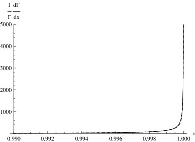
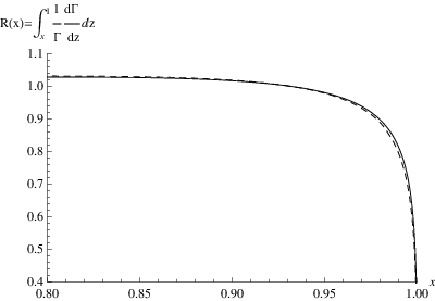
Figure 3: Frozen coupling approx.: top decay jet rates (on the left) and partially integrated jet rates (on the right). Comparison between massless (continuous line) and massive (dashed line) distributions.
Refer to caption
Refer to caption
Figure 4: Frozen coupling approx.: bottom decay jet rates (on the left) and partially integrated jet rates (on the right). Comparison between massless (continuous line) and massive (dashed line) distributions.

It has been already mentioned that there are two ways, analytical and numerical, to compute the inverse Mellin transforms of JN​(Q2,r)J_{N}(Q^{2};r). By numerical method we mean the direct numerical integration in Eq. (47); by analytical method we mean to use the approximated analytical expression for the convolution in Eq. (3.2). In the frozen coupling case, the gig_{i} and did_{i} are linear in λ\lambda and therefore the numerical path does not include the Landau pole; the numerical integration becomes therefore exact.

In figs. 3-4 we compare the (normalized) resummed massless and massive jet rates, in the frozen coupling approximation, for top to b and for b to c decays, respectively. We obtain the same results by calculating the jet factor with both numerical and analytical methods.

5 Resumming with a running coupling constant

Refer to caption
Figure 5: Top decay jet rates: the massive case (dashed line) compared to the massless case (continuous line) at NNLL; αs\alpha_{s} is set to the top mass scale, αs=0.11\alpha_{s}=0.11.
Refer to caption
Figure 6: B decay jet rates: the massive case (dashed line) compared to the massless case (continuous line) at NNLL; αs\alpha_{s} is set to the beauty mass scale, αs=0.219\alpha_{s}=0.219.
Refer to caption
Figure 7: Comparison between the frozen coupling (lighter/red lines) and the running coupling case (thicker/black lines) in B decay jet rates. The dashed (continuous) lines refers the massive (massless) case, at NNLL and with αs=0.23\alpha_{s}=0.23.

By releasing the frozen coupling approximation, we can calculate the distribution with a running coupling. We need in this case a regularization procedure. Indeed, in the massive case, we have four poles on the real axis of the Mellin complex plane respectively for λ=12\lambda=\frac{1}{2}, λ=1\lambda=1 and for ρ=12\rho=\frac{1}{2}, ρ=1\rho=1. These poles arise from the two logarithmic structures of the massless and massive correction formulas. The important point is that the massive poles stand to the right of the massless ones, therefore allowing to use the MP procedure of Ref. [9]. We have integrated numerically Eq. (47), over the path made by two straight lines parallel to the negative real axis, closed by a half-circle centered around the origin and crossing the positive axis between the origin and the first Landau pole. The integrated expression is computed at NNLL order, releasing the frozen coupling approximation; the coupling runs over the whole integration range.

In fig. 5 we compare the resummed massless and massive jet rates for the case of tt to bb decays. All the plots in this section are not normalized. The massless plots coincide, in the considered range, with the ones obtained by the analytical distribution of Eq. (23). Differences between massless and massive case start, as expected, approximately for values of x≃1−r≃0.999x\simeq 1-r\simeq 0.99933 3 We have, approximately, zN−1−1∼−θ⁡(1−z−1/N)z^{N-1}-1\sim-\theta(1-z-1/N) [13], and we can set x≤1−1/N≃1−r.x\leq 1-1/N\simeq 1-r.. We have only listed the NNLL plots, since they do not differ, substantially, with respect to NLL ones. The MP does not avoid approaching to the essentially non-perturbative regime at x≃1x\simeq 1, where the plots start to oscillate and, therefore, a physically motivated treatment of non-perturbative effects has to be introduced. We find that this physical non perturbative cut-off can be put, in practice, equal to 1 in top decay.

In the b decay case (fig. 6), the two curves start differentiating at x≃1−r≃0.9x\simeq 1-r\simeq 0.9, and the difference is visible, with the massive case being less divergent, as expected. The rates in the curves are not normalized, and the NNLL plot presents relevant difference from the NLL one; the addition of NNLL terms renders the plot closer in the rising behavior to the massless plot. At NNLL order we deal not only with double logarithms, but also with single logarithms that shift the position of the minimum 44 4 see f.i. formula (62) in [7].. The effect of the running coupling, affecting in a very distinct manner the massless and the massive case, can be observed by comparing with fig. 4. In order to facilitate the comparison with the frozen coupling case, we report both the massless and massive distributions, not normalized, with frozen and running couplings, in fig. 7.

6 Conclusions

In this paper we have considered the application of the MP to the resummed jet function distributions for heavy quark decays in massless and massive final quarks. We have used a QCD resummation formula in αs\alpha_{s}, that takes into account contribution from large collinear and soft logarithms near the threshold region [8]. Benefits of large threshold logarithms resummation are restoring predictive power to the perturbation series and increase theoretical accuracy, f.i. by a reduction of scale uncertainty. Accuracy is obviously increased by including higher order terms in the exponent. We have considered NNLL order corrections. In the case of massive final quarks, we have analyzed the applicability of the Minimal Prescription scheme to deal with the unavoidable problem, connected with any physical application of QCD resumming formulas, of the integration over the Landau pole.

We calculated the form factors in Mellin and physical space, in order to extract the main and universal features of the perturbative distributions, common to all processes at the threshold. We consider this a necessary first step to approach the phenomenological study of specific decay rates in the QCD resummed framework. In order to compare with data, the further step is to match the distribution with a fixed order coefficient function and include non perturbative effects [21]

As a final remark, let us notice that a very interesting application is to the inclusive semi-leptonic bb decay into cc. In such partonic three body decay, one can combine the resummed with the full triple differential distribution.

We have considered top quark decays, for the recently increased interest due to the large amount of data available at the hadronic machines. One possible application of the present results is to explore the effects of the resummation on the calculation of helicity fractions of the W boson from top quark decays. These are presently measured with increasing precision by both the CDF and the D0 collaboration at the Tevatron.

7 Acknowledgements

We would like to thank U. Aglietti and G. Corcella for very useful discussions. One of us (L.D.G.) thanks the Fondazione A. Della Riccia (Firenze) for financial support and the Theory Group at SLAC for their warm hospitality.

8 Appendix

In this appendix we enlist notations and actual values used in the paper.

The functions g1g_{1} and g2g_{2} introduced in section (2.1) have the following expressions [20]:

g1​(λ,μ2Q2)\displaystyle g_{1}\left(\lambda;\frac{\mu^{2}}{Q^{2}}\right) =\displaystyle= −A12​β0​1λ​[(1−2​λ)​log⁡(1−2​λ)−2​(1−λ)​log⁡(1−λ)];\displaystyle-\frac{A_{1}}{2\beta_{0}}\,\frac{1}{\lambda}\left[\left(1-2\lambda\right)\log\left(1-2\lambda\right)-2\left(1-\lambda\right)\log\left(1-\lambda\right)\right];
g2​(λ,μ2Q2)\displaystyle\,g_{2}\left(\lambda;\frac{\mu^{2}}{Q^{2}}\right) =\displaystyle= +A22​β02​[log⁡(1−2​λ)−2​log⁡(1−λ)]+A1​γEβ0​[log⁡(1−2​λ)−log⁡(1−λ)]+\displaystyle+\frac{A_{2}}{2\beta_{0}^{2}}\left[\log(1-2\lambda)-2\log(1-\lambda)\right]+\frac{A_{1}\gamma_{E}}{\beta_{0}}\left[\log(1-2\lambda)-\log(1-\lambda)\right]+
−β1​A14​β03​[log2⁡(1−2​λ)−2​log2⁡(1−λ)+2​log⁡(1−2​λ)−4​log⁡(1−λ)]+\displaystyle-\frac{\beta_{1}A_{1}}{4\beta_{0}^{3}}\left[\log^{2}(1-2\lambda)-2\log^{2}(1-\lambda)+2\log(1-2\lambda)-4\log(1-\lambda)\right]+
+D12​β0​log⁡(1−2​λ)+B1β0​log⁡(1−λ)+A12​β0​[log⁡(1−2​λ)−2​log⁡(1−λ)]​log​μ2Q2\displaystyle+\frac{D_{1}}{2\beta_{0}}\log(1-2\lambda)+\frac{B_{1}}{\beta_{0}}\log(1-\lambda)+\frac{A_{1}}{2\beta_{0}}\,\left[\log\left(1-2\lambda\right)-2\log\left(1-\lambda\right)\right]\log\frac{\mu^{2}}{Q^{2}}

The NNLO function g3\,g_{3} [19] reads:

g3​(λ,μ2Q2)\displaystyle g_{3}\left(\lambda;\frac{\mu^{2}}{Q^{2}}\right) =\displaystyle= −A32​β02​[λ1−2​λ−λ1−λ]−A1​ζ22​[4​λ1−2​λ−λ1−λ]+\displaystyle-\frac{A_{3}}{2\beta_{0}^{2}}\left[\frac{\lambda}{1-2\lambda}-\frac{\lambda}{1-\lambda}\right]-\frac{A_{1}\zeta_{2}}{2}\left[\frac{4\lambda}{1-2\lambda}-\frac{\lambda}{1-\lambda}\right]+
−A1​β24​β03​[2​λ1−2​λ−2​λ1−λ+2​log⁡(1−2​λ)−4​log⁡(1−λ)]+\displaystyle-\frac{A_{1}\beta_{2}}{4\beta_{0}^{3}}\left[\frac{2\lambda}{1-2\lambda}-\frac{2\lambda}{1-\lambda}+2\log\left(1-2\lambda\right)-4\log\left(1-\lambda\right)\right]+
+A2​β12​β03​[log⁡(1−2​λ)1−2​λ−2​log⁡(1−λ)1−λ+3​λ1−2​λ−3​λ1−λ]+\displaystyle+\frac{A_{2}\beta_{1}}{2\beta_{0}^{3}}\left[\frac{\log\left(1-2\lambda\right)}{1-2\lambda}-\frac{2\log\left(1-\lambda\right)}{1-\lambda}+\frac{3\lambda}{1-2\lambda}-\frac{3\lambda}{1-\lambda}\right]+
−A1​β122​β04[12log2⁡(1−2​λ)1−2​λ−log2⁡(1−λ)1−λ+log⁡(1−2​λ)1−2​λ+\displaystyle-\frac{A_{1}\beta_{1}^{2}}{2\beta_{0}^{4}}\left[\frac{1}{2}\frac{\log^{2}\left(1-2\lambda\right)}{1-2\lambda}-\frac{\log^{2}\left(1-\lambda\right)}{1-\lambda}+\frac{\log\left(1-2\lambda\right)}{1-2\lambda}+\right.
−2​log⁡(1−λ)1−λ+λ1−2​λ−λ1−λ−log(1−2λ)+2log(1−λ)]+\displaystyle\left.-\frac{2\log\left(1-\lambda\right)}{1-\lambda}+\frac{\lambda}{1-2\lambda}-\frac{\lambda}{1-\lambda}-\log\left(1-2\lambda\right)+2\log\left(1-\lambda\right)\right]+
+D1​β12​β02​[log⁡(1−2​λ)1−2​λ+2​λ1−2​λ]+B1​β1β02​[log⁡(1−λ)1−λ+λ1−λ]+\displaystyle+\frac{D_{1}\beta_{1}}{2\beta_{0}^{2}}\left[\frac{\log\left(1-2\lambda\right)}{1-2\lambda}+\frac{2\lambda}{1-2\lambda}\right]+\frac{B_{1}\beta_{1}}{\beta_{0}^{2}}\left[\frac{\log\left(1-\lambda\right)}{1-\lambda}+\frac{\lambda}{1-\lambda}\right]+
−D2β0​λ1−2​λ−B2β0​λ1−λ−A1​γE22​[4​λ1−2​λ−λ1−λ]+\displaystyle-\frac{D_{2}}{\beta_{0}}\frac{\lambda}{1-2\lambda}-\frac{B_{2}}{\beta_{0}}\frac{\lambda}{1-\lambda}-\frac{A_{1}\gamma_{E}^{2}}{2}\left[\frac{4\lambda}{1-2\lambda}-\frac{\lambda}{1-\lambda}\right]+
+A1​β1​γEβ02​[log⁡(1−2​λ)1−2​λ−log⁡(1−λ)1−λ+11−2​λ−11−λ]+\displaystyle+\frac{A_{1}\beta_{1}\gamma_{E}}{\beta_{0}^{2}}\left[\frac{\log\left(1-2\lambda\right)}{1-2\lambda}-\frac{\log\left(1-\lambda\right)}{1-\lambda}+\frac{1}{1-2\lambda}-\frac{1}{1-\lambda}\right]+
−A2​γEβ0​[11−2​λ−11−λ]−D1​γE​2​λ1−2​λ−B1​γE​λ1−λ+\displaystyle-\frac{A_{2}\gamma_{E}}{\beta_{0}}\left[\frac{1}{1-2\lambda}-\frac{1}{1-\lambda}\right]-\frac{D_{1}\gamma_{E}2\lambda}{1-2\lambda}-\frac{B_{1}\gamma_{E}\lambda}{1-\lambda}+
−A12​β0​[2​λ21−2​λ−λ21−λ]​log2​μ2Q2−A2β02​[λ1−2​λ−λ1−λ]​log⁡μ2Q2+\displaystyle-\frac{A_{1}}{2\beta_{0}}\left[\frac{2\lambda^{2}}{1-2\lambda}-\frac{\lambda^{2}}{1-\lambda}\right]\log^{2}\frac{\mu^{2}}{Q^{2}}-\frac{A_{2}}{\beta_{0}^{2}}\left[\frac{\lambda}{1-2\lambda}-\frac{\lambda}{1-\lambda}\right]\log\frac{\mu^{2}}{Q^{2}}+
−A1​γEβ0​[2​λ1−2​λ−λ1−λ]​log⁡μ2Q2−D1β0​λ1−2​λ​log⁡μ2Q2−B1β0​λ1−λ​log⁡μ2Q2+\displaystyle-\frac{A_{1}\gamma_{E}}{\beta_{0}}\left[\frac{2\lambda}{1-2\lambda}-\frac{\lambda}{1-\lambda}\right]\log\frac{\mu^{2}}{Q^{2}}-\frac{D_{1}}{\beta_{0}}\frac{\lambda}{1-2\lambda}\log\frac{\mu^{2}}{Q^{2}}-\frac{B_{1}}{\beta_{0}}\frac{\lambda}{1-\lambda}\log\frac{\mu^{2}}{Q^{2}}+
+A1​β1β03[λ​log⁡(1−2​λ)1−2​λ−λ​log⁡(1−λ)1−λ+λ1−2​λ+\displaystyle+\frac{A_{1}\beta_{1}}{\beta_{0}^{3}}\left[\frac{\lambda\log\left(1-2\lambda\right)}{1-2\lambda}-\frac{\lambda\log\left(1-\lambda\right)}{1-\lambda}+\frac{\lambda}{1-2\lambda}+\right.
−λ1−λ+12log(1−2λ)−log(1−λ)]logμ2Q2.\displaystyle\left.-\frac{\lambda}{1-\lambda}+\frac{1}{2}\log(1-2\lambda)-\log(1-\lambda)\right]\log\frac{\mu^{2}}{Q^{2}}.

Arbitrary constants have been added to the function g3g_{3} in order to make it homogenous. The quantity γE=0.577216​…\gamma_{E}=0.577216\ldots is the Euler constant and ζ⁡(n)\zeta\left(n\right) is the Riemann zeta function,

ζ⁡(n)≡∑k=1∞1kn.\zeta\left(n\right)\equiv\sum_{k=1}^{\infty}\frac{1}{k^{n}}.

ζ⁡(2)=π2/6=1.64493.\zeta\left(2\right)=\pi^{2}/6=1.64493. The functions g2g_{2} and g3g_{3} depend on the renormalization scale μ,\mu, while g1g_{1} does not.

The known values for the resummation constants defined in section (2.1) read:

A1\displaystyle A_{1} =\displaystyle= CFπ;\displaystyle\frac{C_{F}}{\pi};
A2\displaystyle A_{2} =\displaystyle= CFπ2​[CA​(6736−z⁡(2)2)−518​nf];\displaystyle\frac{C_{F}}{\pi^{2}}\left[C_{A}\left(\frac{67}{36}-\frac{z(2)}{2}\right)-\frac{5}{18}n_{f}\right];
A3\displaystyle A_{3} =\displaystyle= CFπ3[CA2(24596+1124z(3)−6736z(2)+118z(4))+\displaystyle\frac{C_{F}}{\pi^{3}}\Bigg[C_{A}^{2}\Big(\,\frac{245}{96}+\frac{11}{24}z(3)-\frac{67}{36}\,z(2)+\frac{11}{8}\,z(4)\Big)\,+
−\displaystyle- CA​nf​(209432+712​z​(3)−518​z​(2))+\displaystyle\,C_{A}\,n_{f}\Big(\frac{209}{432}+\frac{7}{12}z(3)-\frac{5}{18}\,z(2)\Big)+
−\displaystyle- CFnf(5596−z⁡(3)2)−nf2108];\displaystyle\,C_{F}\,n_{f}\Big(\frac{55}{96}-\frac{z(3)}{2}\Big)-\frac{n_{f}^{2}}{108}\Bigg];
B1\displaystyle B_{1} =\displaystyle= −34​CFπ;\displaystyle-\frac{3}{4}\frac{C_{F}}{\pi};
B2\displaystyle B_{2} =\displaystyle= CFπ2[CA(−3155864+1112z(2)+52z(3))+\displaystyle\frac{C_{F}}{\pi^{2}}\Bigg[C_{A}\left(-\frac{3155}{864}+\frac{11}{12}\,z(2)+\frac{5}{2}\,z(3)\right)\,+
−\displaystyle- CF​(332+32​z​(3)−34​z​(2))+\displaystyle C_{F}\left(\frac{3}{32}+\frac{3}{2}z(3)-\frac{3}{4}\,z(2)\right)\,+
+\displaystyle+ nf(247432−z⁡(2)6)];\displaystyle n_{f}\left(\frac{247}{432}-\frac{z(2)}{6}\right)\Bigg];
D1\displaystyle D_{1} =\displaystyle= −CFπ;\displaystyle-\frac{C_{F}}{\pi};
D2\displaystyle D_{2} =\displaystyle= CFπ2​[CA​(55108−94​z​(3)+z⁡(2)2)+nf54],\displaystyle\frac{C_{F}}{\pi^{2}}\left[C_{A}\left(\frac{55}{108}-\frac{9}{4}z(3)+\frac{z(2)}{2}\right)+\frac{n_{f}}{54}\right],

where CA=Nc=3C_{A}=N_{c}=3 is the Casimir of the adjoint representation.

The knowledge of the quantities A1A_{1}, A2A_{2}, B1B_{1} and D1D_{1} is needed for resummation at next-to-leading order.

The coefficients A1A_{1}, B1B_{1} and D1D_{1} are renormalization-scheme independent, as they can be obtained from tree-level amplitudes with one-gluon emission. The higher-order coefficients are instead renormalization-scheme dependent and are given in the M​S¯\overline{MS} scheme for the coupling constant 55 5 A discussion about the scheme dependence of the higher order coefficients A2,B2,A_{2},\,B_{2}, etc. on the coupling constant can be found in [14]..

The coefficients did_{i}, defined in section (2.2), are :

d1​(ρ)\displaystyle d_{1}(\rho) =\displaystyle= A12​β0​ρ​[(1−2​ρ)​log⁡(1−2​ρ)−2​(1−ρ)​log⁡(1−ρ)];\displaystyle\frac{{A_{1}}}{2\,\beta_{0}\,\rho}\Big[\left(1-2\,\rho\right)\,\log(1-2\,\rho)-2\,\left(1-\rho\right)\,\log(1-\rho)\Big];
d2​(ρ)\displaystyle d_{2}(\rho) =\displaystyle= D12​β0​log⁡(1−2​ρ)−B1β0​log⁡(1−ρ)−A22​β02​[log⁡(1−2​ρ)−2​log⁡(1−ρ)]+\displaystyle\frac{{D_{1}}}{2\,{{\beta}_{0}}}\log(1-2\,\rho)-\frac{B_{1}}{{\beta}_{0}}\,\log(1-\rho)-\frac{{A_{2}}}{2\,{{\beta}_{0}}^{2}}\,\Big[\log(1-2\,\rho)-2\,\log(1-\rho)\Big]+
+\displaystyle+ A1​β14​β03​[2​log⁡(1−2​ρ)+log2⁡(1−2​ρ)−4​log⁡(1−ρ)−2​log2⁡(1−ρ)]+\displaystyle\frac{{A_{1}}\,{{\beta}_{1}}}{4\,{{{\beta}_{0}}}^{3}}\,\Big[2\,\log(1-2\,\rho)+{\log^{2}(1-2\,\rho)}-4\,\log(1-\rho)-2\,{\log^{2}(1-\rho)}\Big]\,+
−\displaystyle- A1​γEβ0​[log⁡(1−2​ρ)−log⁡(1−ρ)]−A12​β0​[log⁡(1−2​ρ)−2​log⁡(1−ρ)]​log​μ2m2.\displaystyle\frac{{A_{1}}\,{{\gamma}_{E}}}{{{\beta}_{0}}}\,\Big[\log(1-2\,\rho)-\log(1-\rho)\Big]-\frac{A_{1}}{2\,\beta_{0}}\Big[\log(1-2\,\rho)-2\,\log(1-\rho)\Big]\,\log\frac{\mu^{2}}{m^{2}}.

For the NNLO function d3d_{3} we obtain:

d3​(ρ)\displaystyle d_{3}(\rho) =\displaystyle= −D2β0​ρ1−2​ρ−D1​γE​2​ρ1−2​ρ+D1​β12​β02​[2​ρ1−2​ρ+log⁡(1−2​ρ)1−2​ρ]+\displaystyle-\,\frac{D_{2}}{\beta_{0}}\,\frac{\rho}{1-2\,\rho}\,-\,D_{1}\,\gamma_{E}\,\frac{2\,\rho}{1-2\,\rho}+\frac{{D_{1}}\,{\beta_{1}}}{2\,{{\beta_{0}}}^{2}}\,\left[\frac{2\,\rho}{1-2\,\rho}+\frac{\log(1-2\,\rho)}{1-2\,\rho}\right]\,+
+\displaystyle+ B2β0​ρ1−ρ+B1​γE​ρ1−ρ+\displaystyle\frac{B_{2}}{\beta_{0}}\,\frac{\rho}{1-\rho}\,+\,B_{1}\,\gamma_{E}\,\frac{\rho}{1-\rho}\,+
−\displaystyle- B1​β1β02​[ρ1−ρ+log⁡(1−ρ)1−ρ]+A32​β02​[ρ1−2​ρ−ρ1−ρ]+\displaystyle\frac{B_{1}\,\beta_{1}}{{\beta_{0}}^{2}}\,\left[\frac{\rho}{1-\rho}+\frac{\log(1-\rho)}{1-\rho}\right]+\frac{A_{3}}{2\,{{\beta_{0}}}^{2}}\,\left[\frac{\rho}{1-2\,\rho}-\frac{\rho}{1-\rho}\right]+
+\displaystyle+ A2​γEβ0​[2​ρ1−2​ρ−ρ1−ρ]+\displaystyle\frac{A_{2}\,{\gamma_{E}}}{{\beta_{0}}}\,\left[\frac{2\,\rho}{1-2\,\rho}-\frac{\rho}{1-\rho}\right]+
−\displaystyle- A2​β12​β03​[3​ρ1−2​ρ−3​ρ1−ρ+log⁡(1−2​ρ)1−2​ρ−2​log⁡(1−ρ)1−ρ]+\displaystyle\frac{A_{2}\,\beta_{1}}{2\,{\beta_{0}}^{3}}\,\left[\frac{3\,\rho}{1-2\,\rho}-\frac{3\,\rho}{1-\rho}+\frac{\log(1-2\,\rho)}{1-2\,\rho}-\frac{2\,\log(1-\rho)}{1-\rho}\right]+
+\displaystyle+ A1​γE22​[4​ρ1−2​ρ−ρ1−ρ]+A1​π212​[4​ρ1−2​ρ−ρ1−ρ]+\displaystyle\frac{A_{1}\,{\gamma_{E}}^{2}}{2}\,\left[\frac{4\,\rho}{1-2\,\rho}-\frac{\rho}{1-\rho}\right]+\frac{A_{1}\,{\pi}^{2}}{12}\,\left[\frac{4\,\rho}{1-2\,\rho}-\frac{\rho}{1-\rho}\right]+
+\displaystyle+ A1​β24​β03​[2​ρ1−2​ρ−2​ρ1−ρ+2​log⁡(1−2​ρ)−4​log⁡(1−ρ)]+\displaystyle\frac{A_{1}\,\beta_{2}}{4\,{\beta_{0}}^{3}}\,\left[\frac{2\,\rho}{1-2\,\rho}-\frac{2\,\rho}{1-\rho}+2\,\log(1-2\,\rho)-4\,\log(1-\rho)\right]+
−\displaystyle- A1​β1​γEβ02​[2​ρ1−2​ρ−ρ1−ρ+log⁡(1−2​ρ)1−2​ρ−log⁡(1−ρ)1−ρ]+\displaystyle\frac{A_{1}\,\beta_{1}\,\gamma_{E}}{{\beta_{0}}^{2}}\,\left[\frac{2\,\rho}{1-2\,\rho}-\frac{\rho}{1-\rho}+\frac{\log(1-2\,\rho)}{1-2\,\rho}-\frac{\log(1-\rho)}{1-\rho}\right]+
+\displaystyle+ A1​β122​β04[ρ1−2​ρ−ρ1−ρ−log(1−2ρ)+log⁡(1−2​ρ)1−2​ρ\displaystyle\frac{A_{1}\,{\beta_{1}}^{2}}{2\,{\beta_{0}}^{4}}\,\left[\frac{\rho}{1-2\,\rho}-\frac{\rho}{1-\rho}-\log(1-2\,\rho)+\frac{\log(1-2\,\rho)}{1-2\,\rho}\right.
+\displaystyle+ log2⁡(1−2​ρ)2​(1−2​ρ)+2log(1−ρ)−2​log⁡(1−ρ)1−ρ−log2⁡(1−ρ)1−ρ]+\displaystyle\left.\frac{\log^{2}(1-2\,\rho)}{2\,\left(1-2\,\rho\right)}+2\,\log(1-\rho)-\frac{2\,\log(1-\rho)}{1-\rho}-\frac{\log^{2}(1-\rho)}{1-\rho}\right]\,+\,
−\displaystyle- D1β0​ρ1−2​ρ​log⁡μ2m2+B1β0​ρ1−ρ​log⁡μ2m2+A2β02​[ρ1−2​ρ−ρ1−ρ]​log⁡μ2m2+\displaystyle\frac{D_{1}}{\beta_{0}}\frac{\rho}{1-2\,\rho}\,\log\frac{{\mu}^{2}}{m^{2}}+\frac{B_{1}}{\beta_{0}}\frac{\rho}{1-\rho}\,\log\frac{{\mu}^{2}}{m^{2}}+\frac{{A_{2}}}{{{\beta_{0}}}^{2}}\,\left[\frac{\rho}{1-2\,\rho}-\frac{\rho}{1-\rho}\right]\,\log\frac{{\mu}^{2}}{m^{2}}+
+\displaystyle+ A1​γEβ0​[2​ρ1−2​ρ−ρ1−ρ]​log⁡μ2m2+\displaystyle\frac{{A_{1}}\,{\gamma_{E}}}{{\beta_{0}}}\,\left[\frac{2\,\rho}{1-2\,\rho}-\frac{\rho}{1-\rho}\right]\,\log\frac{{\mu}^{2}}{m^{2}}+
−\displaystyle- A1​β1β03[ρ1−2​ρ−ρ1−ρ+log⁡(1−2​ρ)2+ρ​log⁡(1−2​ρ)1−2​ρ+\displaystyle\frac{{A_{1}}{\beta_{1}}}{{{\beta_{0}}}^{3}}\left[\frac{\rho}{1-2\,\rho}-\frac{\rho}{1-\rho}+\frac{\log(1-2\,\rho)}{2}+\frac{{\rho}\,\log(1-2\,\rho)}{1-2\,\rho}\right.+\,
−\displaystyle- log(1−ρ)−ρ​log⁡(1−ρ)1−ρ]logμ2m2+\displaystyle\left.\log(1-\rho)-\frac{\rho\,\log(1-\rho)}{1-\rho}\right]\log\frac{{\mu}^{2}}{m^{2}}\!+
+\displaystyle+ A12​β0​[2​ρ21−2​ρ−ρ21−ρ]​log2​μ2m2.\displaystyle\frac{{A_{1}}}{2\,{\beta_{0}}}\,\left[\frac{2\,{\rho}^{2}}{1-2\,\rho}-\frac{{\rho}^{2}}{1-\rho}\right]\,{\log^{2}\frac{{\mu}^{2}}{m^{2}}}.

The coefficients βi\beta_{i} of the QCD β\beta-function in our normalization have been given in [7].

References

  • [1] G. Parisi and R. Petronzio, Nucl. Phys. B 154, 427 (1979); G. Curci and M. Greco, Phys. Lett. B92, 175 (1980).
  • [2] J. Kodaira and L. Trentadue, SLAC-PUB-2934 (1982); Phys. Lett. B 112, 66 (1982); S. Catani, E. D’Emilio and L. Trentadue, Phys. Lett. B 211, 335 (1988).
  • [3] S. Catani and L. Trentadue, Nucl. Phys. B 327, 323 (1989).
  • [4] S. Catani and L. Trentadue, Nucl. Phys. B 353, 183 (1991).
  • [5] G. Sterman, Nucl. Phys. B 281, 310 (1987).
  • [6] U. Aglietti, Nucl. Phys. B 610 (2001) 293
  • [7] U. Aglietti, G. Ricciardi and G. Ferrera, Phys. Rev. D 74 (2006) 034004
  • [8] U. Aglietti, L. Di Giustino, G. Ferrera and L. Trentadue, Phys. Lett. B 651 (2007) 275.
  • [9] S. Catani, M. Mangano, P. Nason and L. Trentadue, Nucl. Phys. B 478 (1996) 273.
  • [10] P. Gambino, C. Schwanda, [arXiv:1102.0210 [hep-ex]].
  • [11] M. Cacciari, G. Corcella and A. D. Mitov, JHEP 0212 (2002) 015.
  • [12] M. Cacciari and S. Catani, Nucl. Phys. B 617 (2001) 253.
  • [13] S. Catani and L. Trentadue, Nucl. Phys. B 327 (1989) 323.
  • [14] S. Catani, B. R. Webber and G. Marchesini, Nucl. Phys. B 349 (1991) 635.
  • [15] U. Aglietti, R. Sghedoni and L. Trentadue, Phys. Lett. B 522 (2001) 83; Phys. Lett. B 585 (2004) 131.
  • [16] S. Moch and A. Vogt, Phys. Lett. B 631 (2005) 48
  • [17] J.  Kodaira and L. Trentadue, Phys. Lett. B 112 (1982) 66.
  • [18] A. Vogt, Phys. Lett. B 497 (2001) 228.
  • [19] U. Aglietti and G. Ricciardi, Phys. Rev. D 66 (2002) 074003
  • [20] R. Akhouri and I. Rothstein, Phys. Rev. D 54 (1996) 2349; G. Korchemsky and G. Sterman, Phys. Lett. B 340 (1994) 96.
  • [21] L. Di Giustino, G. Ricciardi and L. Trentadue, in preparation.