跳到论文正文
W Papers独立论文阅读器 arXiv:1102.0238 论文正文 计算阅读时间 · 0%
引用这篇论文根据当前论文元数据生成,正式投稿前建议核对。


License: arXiv.org perpetual non-exclusive license
arXiv:1102.0238v2 [math-ph] 03 Mar 2011

Coherent electromagnetic wavelets and their twisting null congruences

Gerald Kaiser Affiliation: Center for Signals and Waves Affiliation: Austin, TX Affiliation: kaiser@wavelets.com ∙\bullet www.wavelets.com
Abstract

We construct an electromagnetic field whose scalar potential is a pulsed-beam wavelet Ψ~{\tilde{\Psi}} (an analytic continuation of a classical Huygens wavelet). The vector potential 𝐀~{\bf{\tilde{A}}} is determined up to three complex parameters by requiring that (a) it satisfies the Lorenz gauge condition with Ψ~{\tilde{\Psi}}, (b) its current density is supported on the same disk 𝒟{\mathcal{D}} as the charge density of Ψ~{\tilde{\Psi}}, (c) it is axisymmetric, and (d) it has the same retarded time dependence as Ψ~{\tilde{\Psi}}. By choosing one of the parameters in 𝐀~{\bf{\tilde{A}}} appropriately, the electromagnetic field generated by the four-potential (𝐀~,Ψ~)({\bf{\tilde{A}}},{\tilde{\Psi}}) can be made null, meaning that 𝑬2=𝑩2{\boldsymbol{E}}^{2}={\boldsymbol{B}}^{2} and 𝑬⋅𝑩=0{\boldsymbol{E}}\cdot{\boldsymbol{B}}=0. We call such fields coherent because upon being radiated, they do not loiter around the source, generating electromagnetic inertia, but immediately propagate out at the speed of light. The coherent EM wavelets define a twisting null congruence of light rays in Minkowski space, which we show to be identical to the Kerr congruence associated with the Kerr-Newman metric. The latter represents a black hole due to a time-independent charge-current density on a massive disk 𝒟{\mathcal{D}} spinning at the angular velocity c/ac/a, where aa is the radius of 𝒟{\mathcal{D}}. By contrast, our coherent wavelets are electromagnetic pulsed beams radiated by pulsed charge-current distributions on 𝒟{\mathcal{D}}, still spinning at the uniform rate c/ac/a.

1 The inertia density of an electromagnetic field

The energy density uu and the Poynting vector 𝑺{\boldsymbol{S}} of an electromagnetic field (𝑬,𝑩)({\boldsymbol{E}},{\boldsymbol{B}}) in vacuum are given by

u⁡(x)=12​(𝑬​(x)2+𝑩​(x)2)and𝑺⁡(x)=𝑬⁡(x)×𝑩⁡(x),\displaystyle u{(x)}=\frac{1}{2}({\boldsymbol{E}}{(x)}^{2}+{\boldsymbol{B}}{(x)}^{2})\ \ \hbox{and}\ \ {\boldsymbol{S}}{(x)}={\boldsymbol{E}}{(x)}\times{\boldsymbol{B}}{(x)}, (1)

where x=(𝒙,t)∈ℝ4x=({\boldsymbol{x}},t)\in{{\mathbb{R}}^{4}} are the spacetime variables. We are using Heaviside-Lorentz units (ε0=μ0=1)(\varepsilon_{0}=\mu_{0}=1). 𝑺{\boldsymbol{S}} satisfies the vector identity

𝑺2=𝑬2​𝑩2−(𝑬⋅𝑩)2,\displaystyle{\boldsymbol{S}}^{2}={\boldsymbol{E}}^{2}{\boldsymbol{B}}^{2}-({\boldsymbol{E}}\cdot{\boldsymbol{B}})^{2},

which implies that

u2−𝑺2=14​(𝑬2−𝑩2)2+(𝑬⋅𝑩)2≥0.\displaystyle u^{2}-{\boldsymbol{S}}^{2}=\frac{1}{4}({\boldsymbol{E}}^{2}-{\boldsymbol{B}}^{2})^{2}+({\boldsymbol{E}}\cdot{\boldsymbol{B}})^{2}\geq 0. (2)

The electromagnetic momentum density is given by11 1 In SI units [J99, page 261], 𝒈=𝑺/c2{\boldsymbol{g}}={\boldsymbol{S}}/c^{2}.

𝒈⁡(x)=𝑺⁡(x)/c,\displaystyle{\boldsymbol{g}}{(x)}={\boldsymbol{S}}{(x)}/c\,,

where cc is the speed of light. For a relativistic particle with energy EE and momentum 𝒑{\boldsymbol{p}}, the mass and velocity are given by

m2​c4=E2−c2​𝒑2≥0and𝒗=c2​𝒑E⇒𝒗2≤c2.\displaystyle m^{2}c^{4}=E^{2}-c^{2}{\boldsymbol{p}}^{2}\geq 0\ \ \hbox{and}\ \ {\boldsymbol{v}}=\frac{c^{2}{\boldsymbol{p}}}{E}\ \Rightarrow\ {\boldsymbol{v}}^{2}\leq c^{2}. (3)

Thus it makes sense to define the electromagnetic inertia density

ℐ⁡(x)=c−2​u​(x)2−c2​𝒈​(x)2=12​c2​(𝑬2−𝑩2)2+4​(𝑬⋅𝑩)2\displaystyle\boxed{\ {\mathcal{I}}{(x)}=c^{-2}\sqrt{u{(x)}^{2}-c^{2}{\boldsymbol{g}}{(x)}^{2}}=\frac{1}{2c^{2}}\sqrt{({\boldsymbol{E}}^{2}-{\boldsymbol{B}}^{2})^{2}+4({\boldsymbol{E}}\cdot{\boldsymbol{B}})^{2}}\ } (4)

and the electromagnetic energy flow velocity

𝒗(x)=c​𝑺​(x)u⁡(x),𝒗(x)2≤c2.\displaystyle\boxed{\ {\boldsymbol{v}}{(x)}=\frac{c{\boldsymbol{S}}{(x)}}{u{(x)}},\quad{\boldsymbol{v}}{(x)}^{2}\leq c^{2}.\ } (5)

ℐ⁡(x){\mathcal{I}}{(x)} and 𝒗⁡(x){\boldsymbol{v}}{(x)} are local spacetime fields. Since 𝑬2−𝑩2{\boldsymbol{E}}^{2}-{\boldsymbol{B}}^{2} and 𝑬⋅𝑩{\boldsymbol{E}}\cdot{\boldsymbol{B}} are Lorentz-invariant, ℐ⁡(x){\mathcal{I}}{(x)} is a scalar field.

From here on we set

c≡1,\displaystyle c\equiv 1,

although cc will be inserted into expressions occasionally to clarify their physical contents.

The energy, momentum and inertia densities of a field can be expressed succinctly in terms of the complex vector fields

𝑭⁡(x)=𝑬⁡(x)+i​𝑩​(x)\displaystyle{\boldsymbol{F}}{(x)}={\boldsymbol{E}}{(x)}+i{\boldsymbol{B}}{(x)} (6)

as follows:

2​u=𝑭∗⋅𝑭=|𝑭|2\displaystyle 2u={\boldsymbol{F}}^{*}\cdot{\boldsymbol{F}}=|{\boldsymbol{F}}|^{2} 2​i​𝑺=𝑭∗×𝑭\displaystyle 2i{\boldsymbol{S}}={\boldsymbol{F}}^{*}\times{\boldsymbol{F}} 2​ℐ=|𝑭2|.\displaystyle 2{\mathcal{I}}=|{\boldsymbol{F}}^{2}|. (7)

The combinations 𝑬±i​𝑩{\boldsymbol{E}}\pm i{\boldsymbol{B}} have been called Riemann-Silberstein vectors [B96] and Faraday vectors [B99]. They have been rediscovered many times and were explored extensively by Bateman [B15]. See also [K94, Chapter 9] and [K4].

By (4),

ℐ⁡(x)=0⇔𝑬​(x)2−𝑩​(x)2=𝑬⁡(x)⋅𝑩⁡(x)=0⇔𝑭2=0.\displaystyle{\mathcal{I}}{(x)}=0\ \Leftrightarrow\ {\boldsymbol{E}}{(x)}^{2}-{\boldsymbol{B}}{(x)}^{2}={\boldsymbol{E}}{(x)}\cdot{\boldsymbol{B}}{(x)}=0\ \Leftrightarrow\ {\boldsymbol{F}}^{2}=0. (8)

An electromagnetic field with 𝑭​(x)2=0{\boldsymbol{F}}{(x)}^{2}=0 is said to be null at xx. Nullity is a local, Lorentz-invariant concept. It is the field counterpart of a massless particle. Indeed,

|𝒗⁡(x)|=1⇔ℐ⁡(x)=0.\displaystyle|{\boldsymbol{v}}{(x)}|=1\ \Leftrightarrow\ {\mathcal{I}}{(x)}=0. (9)

Electromagnetic energy propagates at the speed of light only at events xx where the field is null. Elsewhere, it travels at speeds less than cc and has a positive inertia density.

Although this simple fact should be widely known in classical electrodynamics, I’ve been unable to find any clear reference to it in the mainstream literature and in discussions with several knowledgeable colleagues. The sole exception, to my knowledge, is a brief note in [B15, page 6].22 2 In quantum electrodynamics it is well known that exchanged photons are virtual (off the zero-mass shell in Fourier space), hence they can have any speed – possibly greater than cc. It should be interesting to connect these classical and quantum ideas. They are in some sense dual: one is local in 4D spacetime, and the other is local in 4D Fourier space.

How are we to understand that electromagnetic waves, which are the ingredients of light itself, do not generally travel at the speed of light? The explanation is simple.

∙\bullet\ It is well known that every electromagnetic field becomes asymptotically null in the far zone, where its wavefronts become asymptotic to plane waves. But fields are generally not null in the near zone, close to their sources. Hence a generic electromagnetic field (i.e., one not chosen in a special way) has a non-vanishing inertia density in the near zone which decays to zero in the far zone. This explains why observed light (which is usually seen in the far zone due to its very short wavelength) is seen to propagate at a speed very close to cc.

∙\bullet\ The inertia in the near zone can be understood as the result of interference between different parts of the field. As illustrated in Figure 1, parts of the near field propagate away from the source while other parts propagate back toward the source. That causes reactive energy to circulate back and forth between the source and the near field, giving rise to inertia. This has important consequences in antenna theory, where electromagnetic fields tend to loiter near the antenna to a larger or lesser extent. Antennas generating a great deal of reactive energy are inefficient radiators since the associated inertia tends to slow down their transmission time, effectively limiting the bandwidth. For a careful analysis of the reactive energy in the near zone of antennas, see [Y96]. See also [Wik-NF] for a less rigorous but easily comprehensible description.

∙\bullet\ An important aspect of nullity was discovered by Iwo Bialynicki-Birula [B3]. A generic electromagnetic field in free space is null along a set of 2-dimensional hypersurfaces 𝒮{\mathcal{S}} in spacetime since 𝑭​(𝒙,t)2=0{\boldsymbol{F}}({\boldsymbol{x}},t)^{2}=0 imposes two real conditions on the four spacetime variables (𝒙,t)({\boldsymbol{x}},t). The time-slices 𝒮t{\mathcal{S}}_{t} of 𝒮{\mathcal{S}} are (generically) curves in space, and these curves evolve with tt. Bialynicki-Birula showed that the non-null field surrounding such a curve circulates around it, forming a vortex line along 𝒮t{\mathcal{S}}_{t}. The above argument shows that when a field is not null in an extended region of spacetime, it travels at the speed of light only along such electromagnetic vortices. Elsewhere it travels at speeds less than cc, although the energy flow speed everywhere approaches cc in the far zone.

∙\bullet\ The characteristic property of fields that are null in an extended region of spacetime (not merely on isolated vortex lines, as in the case of a generic field) is that they are coherent, i.e., their various parts travel in unison and without interference. They are rewarded by having zero inertia and propagating at the exact speed cc within the region of coherence.

Figure 1: In the near zone, the energy in a generic wave propagates back to the source as well as away from it. This incoherence leads to reactive energy and an energy flow speed v<cv<c, hence inertia. In the far zone, only the outgoing waves survive and the field becomes asymptotically coherent.

Various classes of globally null electromagnetic fields (where 𝑭2{\boldsymbol{F}}^{2} vanishes almost everywhere, with the possible exception of singularities whose supports have zero measure) are known; for examples, see [B15, R61, T62, RT64]. However, no solutions with extended sources appear to be known which radiate null fields everywhere outside the source region.

In this paper we construct a class of localized pulsed-beam fields whose charge-current densities live on a disk in space and which are null everywhere outside the disk.33 3 More accurately, the fields are also singular on the line forming the axis of the disk, which acts as a vortex jet. See section 9. We call these fields coherent electromagnetic wavelets. If the singular sources radiating such wavelets can be approximated in practice, they should be very efficient radiators.

2 The scalar pulsed-beam wavelets Ψ~​(𝒙,t){\tilde{\Psi}}({\boldsymbol{x}},t)

We now summarize some results regarding pulsed-beam wavelet solutions of the scalar wave equation. Detailed explanations can be found in [K3, HK9].

Consider the wave Ψ⁡(𝒙,t)\Psi({\boldsymbol{x}},t) radiated by the point source 4​π​δ​(𝒙)4\pi\delta({\boldsymbol{x}}) driven by a pulse g0​(t)g_{0}{(t)}, which satisfies the wave equation

□Ψ(𝒙,t)=4πg0(t)δ(𝒙),where□=∂t2−Δ\displaystyle\Box\Psi({\boldsymbol{x}},t)=4\pi g_{0}{(t)}\delta({\boldsymbol{x}}),\ \ \hbox{where}\ \ \Box=\partial_{t}^{2}-\Delta (10)

is the wave operator. The unique causal (retarded) solution is

Ψ⁡(𝒙,t)=g0​(t−r)r≡g0​(t−r/c)r.\displaystyle\Psi({\boldsymbol{x}},t)=\frac{g_{0}(t-r)}{r}\equiv\frac{g_{0}(t-r/c)}{r}. (11)

The corresponding scalar pulsed-beam wavelet Ψ~{\tilde{\Psi}} is an extension of Ψ\Psi to complex spacetime, obtained formally by displacing the point source from the origin to an imaginary point i​𝒂i{\boldsymbol{a}}. It is defined by

Ψ~​(𝒙,t)=g⁡(τ−ζ)ζ\displaystyle{\tilde{\Psi}}({\boldsymbol{x}},t)=\frac{g(\tau-\zeta)}{\zeta} (12)

where τ=t−i​s\tau=t-is is a complex time,

ζ=(𝒙−i​𝒂)2=r2−a2−2​i​𝒂⋅𝒙,r=|𝒙|,a=|𝒂|\displaystyle\zeta=\sqrt{({\boldsymbol{x}}-i{\boldsymbol{a}})^{2}}=\sqrt{r^{2}-a^{2}-2i{\boldsymbol{a}}\cdot{\boldsymbol{x}}},\quad r=|{\boldsymbol{x}}|,\ a=|{\boldsymbol{a}}| (13)

is the complex distance44 4 The idea of transforming a spherically symmetric solution of a partial differential equation with a point source to a cylindrically symmetric one by an imaginary displacement of the point source, and the ensuing complex distance, was introduced by Ted Newman in general relativity in 1965. Newman and his collaborators used it to derive the Kerr solution (neutral spinning black hole) and the Kerr-Newman solution (charged spinning black hole) from the spherically symmetric Schwarzschild and ReissnerÐNordström solutions, respectively [NJ65, N65]. Deschamps discovered the idea independently in 1971 in the context of the Helmholtz equation, where he use it to derive the time-harmonic complex-source beams [D71] from the spherically symmetric Green function, as in (25): ei​k​rr→ei​k​ζζ.\displaystyle\frac{e^{ikr}}{r}\to\frac{e^{ik\zeta}}{\zeta}. Probably the earliest use of ζ\zeta was in 1897, when Appell used it to study the analytically continued Newtonian potential 1/ζ1/\zeta as a harmonic function [A87]. from the imaginary source point i​𝒂i{\boldsymbol{a}} to the real observation point 𝒙{\boldsymbol{x}}, and gg is the analytic signal or positive-frequency part of the driving signal g0​(t)g_{0}{(t)}, i.e.,

g⁡(τ)\displaystyle g(\tau) =12​π​∫0∞d​ω​e−i​ω​τ​g^0​(ω)=12​π​∫0∞d​ω​e−i​ω​t​e−ω​s​g^0​(ω).\displaystyle=\frac{1}{2\pi}\int_{0}^{\infty}{\rm d}\omega\,e^{-i\omega\tau}{\hat{g}}_{0}{(\omega)}=\frac{1}{2\pi}\int_{0}^{\infty}{\rm d}\omega\,e^{-i\omega t}e^{-\omega s}{\hat{g}}_{0}{(\omega)}. (14)

Here g^0​(ω){\hat{g}}_{0}{(\omega)} is the usual Fourier transform. If g0g_{0} is square-integrable, then gg is analytic in the lower-half complex time plane s>0s>0 due to the smoothing factor e−ω​se^{-\omega s} in (14). If g^0​(ω){\hat{g}}_{0}{(\omega)} decays rapidly as ω→∞\omega\to\infty, then g⁡(t−i​s)g(t-is) may also extend analytically into the upper half-plane. For example, in [HK9] we used the Gaussian pulse of duration d>0d>0,

g0​(t)=e−t2/d2π​d,\displaystyle g_{0}{(t)}=\frac{e^{-t^{2}/d^{2}}}{\sqrt{\pi}d}, (15)

so that

d→0⇒Ψ⁡(𝒙,t)→δ⁡(t−r)r.\displaystyle d\to 0\ \Rightarrow\ \Psi({\boldsymbol{x}},t)\to\frac{\delta(t-r)}{r}.

This is the retarded wave propagator, a fundamental solution of the wave equation:

□​Ψ​(𝒙,t)=4​π​δ​(t)​δ​(𝒙).\displaystyle\Box\Psi({\boldsymbol{x}},t)=4\pi\delta{(t)}\delta({\boldsymbol{x}}).

The associated pulsed beams Ψ~​(𝒙,t){\tilde{\Psi}}({\boldsymbol{x}},t) were shown to form a ‘basis’ for all radiated solutions of the wave equation by extending Huygens’ principle to complex spacetime. Thus Ψ~{\tilde{\Psi}} are ‘wavelets’ in two different senses:

  • •

    From a classical point of view, Ψ~{\tilde{\Psi}} and its spacetime translates Ψ~​(x−x0){\tilde{\Psi}}(x-x_{0}) are pulsed-beam versions of Huygens wavelets. The analytic continuation to complex spacetime breaks the spherical symmetry of the latter, deforming them to pulsed beams.

  • •

    From a modern point of view, they are a family of localized functions paramaterized by their centers and widths which can be used to expand a space of functions, as in time-scale analysis [K94]. In this case, the centers are the real spacetime translation parameters x0x_{0}, the widths are the imaginary translation parameters (𝒂,s)({\boldsymbol{a}},s), and the space of functions represented as superpositions of Ψ~{\tilde{\Psi}} are radiated waves.

Returning to the general wavelet Ψ~{\tilde{\Psi}} in (12), we define its source ϱ~{\tilde{\varrho}} by

4​π​ϱ~​(𝒙,t)=□​Ψ~​(𝒙,t),\displaystyle 4\pi{\tilde{\varrho}}({\boldsymbol{x}},t)=\Box{\tilde{\Psi}}({\boldsymbol{x}},t), (16)

where the wave operator □\Box must act in the distributional sense to accommodate the singularities of Ψ~{\tilde{\Psi}}. To understand ϱ~{\tilde{\varrho}}, note that the complex square root ζ\zeta has branch points whenever its argument belongs to the negative real axis:

r2−a2−2​i​𝒂⋅𝒙≤0⇔r≤aand𝒂⋅𝒙=0.\displaystyle r^{2}-a^{2}-2i{\boldsymbol{a}}\cdot{\boldsymbol{x}}\leq 0\ \Leftrightarrow\ r\leq a\ \ \hbox{and}\ \ {\boldsymbol{a}}\cdot{\boldsymbol{x}}=0.

Since we are keeping the imaginary spacetime variables (𝒂,s)({\boldsymbol{a}},s) fixed, the branch points of ζ\zeta form the disk in ℝ3{{\mathbb{R}}^{3}} given by

𝒟={𝒙:r≤a,𝒂⋅𝒙=0}={𝒙:Reζ=0}.\displaystyle{\mathcal{D}}=\{{\boldsymbol{x}}:r\leq a,\ {\boldsymbol{a}}\cdot{\boldsymbol{x}}=0\}=\{{\boldsymbol{x}}:{\,\rm Re}\ \zeta=0\}. (17)

The formal displacement of the point source from the origin to i​𝒂i{\boldsymbol{a}} transforms the point singularity of Ψ\Psi to a disk singularity of Ψ~{\tilde{\Psi}} on 𝒟{\mathcal{D}}. Ψ~{\tilde{\Psi}} is infinite on the boundary

𝒞=∂𝒟={𝒙:r=a,𝒂⋅𝒙=0}={𝒙:ζ=0}\displaystyle{\mathcal{C}}=\partial{\mathcal{D}}=\{{\boldsymbol{x}}:r=a,\ {\boldsymbol{a}}\cdot{\boldsymbol{x}}=0\}=\{{\boldsymbol{x}}:\zeta=0\} (18)

and discontinuous across the interior of 𝒟{\mathcal{D}}, where Im​ζ{\,\rm Im}\ \zeta has a jump discontinuity. We choose the branch of ζ\zeta with Re​ζ≥0{\,\rm Re}\ \zeta\geq 0, so that ζ\zeta is an extension of the positive Euclidean distance, i.e., ζ→r\zeta\to r as 𝒂→𝟎{\boldsymbol{a}}\to{\boldsymbol{0}}. It then follows that Ψ~{\tilde{\Psi}} is an extension of Ψ\Psi in the sense that (a) its source ϱ~​(𝒙,t){\tilde{\varrho}}({\boldsymbol{x}},t) vanishes whenever 𝒙∉𝒟{\boldsymbol{x}}\notin{\mathcal{D}}, and (b)

𝒂→𝟎,s→0⇒ 2​Re​Ψ~​(𝒙,t)→g0​(t−r)r≡Ψ⁡(𝒙,t).\displaystyle{\boldsymbol{a}}\to{\boldsymbol{0}},\ s\to 0\ \Rightarrow\ 2{\,\rm Re}\ {\tilde{\Psi}}({\boldsymbol{x}},t)\to\frac{g_{0}(t-r)}{r}\equiv\Psi({\boldsymbol{x}},t).

Taking the real part is necessary to restore the negative-frequency component of g0g_{0}. The distribution ϱ~{\tilde{\varrho}} in (16) has been computed rigorously in [K0, K4a].

As its name indicates, Ψ~​(𝒙,t){\tilde{\Psi}}({\boldsymbol{x}},t) is a pulsed beam radiated by the disk 𝒟{\mathcal{D}} and propagating in the direction of 𝒂{\boldsymbol{a}}. To see this, write

ζ=ξ−i​η,ξ≥0.\displaystyle\zeta=\xi-i\eta,\quad\xi\geq 0. (19)

Choosing a cylindrical coordinate system (ρ,ϕ,z)(\rho,\phi,z) with zz-axis parallel to 𝒂{\boldsymbol{a}}, we have

ζ2=(𝒙−i​𝒂)2=r2−a2−2​i​𝒂⋅𝒙=ξ2−η2−2​i​ξ​η,\displaystyle\zeta^{2}=({\boldsymbol{x}}-i{\boldsymbol{a}})^{2}=r^{2}-a^{2}-2i{\boldsymbol{a}}\cdot{\boldsymbol{x}}=\xi^{2}-\eta^{2}-2i\xi\eta,

hence

r2−a2=ξ2−η2anda​z=ξ​η\displaystyle r^{2}-a^{2}=\xi^{2}-\eta^{2}\ \ \hbox{and}\ \ az=\xi\eta

and

a2​ρ2=a2​r2−a2​z2=a2​(a2+ξ2−η2)−ξ2​η2.\displaystyle a^{2}\rho^{2}=a^{2}r^{2}-a^{2}z^{2}=a^{2}(a^{2}+\xi^{2}-\eta^{2})-\xi^{2}\eta^{2}.

Therefore (ξ,η)(\xi,\eta) are related to (ρ,z)(\rho,z) as follows:

a2​ρ2=(a2+ξ2)​(a2−η2)anda​z=ξ​η.\displaystyle\boxed{\ a^{2}\rho^{2}=(a^{2}+\xi^{2})(a^{2}-\eta^{2})\ \ \hbox{and}\ \ az=\xi\eta.\ } (20)

In particular, it follows that

  • •

    0≤ξ≤r0\leq\xi\leq r and −a≤η≤a-a\leq\eta\leq a,

  • •

    the level surfaces of ξ\xi are the oblate spheroids

    𝒪ξ={𝒙:ρ2a2+ξ2+z2ξ2=1},ξ>0,\displaystyle{\mathcal{O}}_{\xi}=\left\{{\boldsymbol{x}}:\frac{\rho^{2}}{a^{2}+\xi^{2}}+\frac{z^{2}}{\xi^{2}}=1\right\},\quad\xi>0, (21)
  • •

    the level surfaces of η\eta are the semi-hyperboloids

    ℋη={𝒙:ρ2a2−η2−z2η2=1,Sgnz=Sgnη},0<η2<a2.\displaystyle{\mathcal{H}}_{\eta}=\left\{{\boldsymbol{x}}:\frac{\rho^{2}}{a^{2}-\eta^{2}}-\frac{z^{2}}{\eta^{2}}=1,\ {\,\rm Sgn\,}z={\,\rm Sgn\,}\eta\right\},\quad 0<\eta^{2}<a^{2}. (22)

The far zone consists of points 𝒙{\boldsymbol{x}} with r≫ar\gg a, where the observer is far from the disk. By (13) and (19),

r≫a⇒ξ≈randη≈𝒂⋅𝐱^≡a​cos⁡θ,𝐱^=𝒙/r.\displaystyle r\gg a\ \Rightarrow\ \xi\approx r\ \ \hbox{and}\ \ \eta\approx{\boldsymbol{a}}\cdot\mbox{\boldmath{{$\rm\hat{x}$}}}\equiv a\cos\theta,\quad\mbox{\boldmath{{$\rm\hat{x}$}}}={\boldsymbol{x}}/r. (23)

Hence ξ\xi is a deformation of rr and η\eta is a deformation of a​cos⁡θa\cos\theta. For ξ≫a\xi\gg a, 𝒪ξ{\mathcal{O}}_{\xi} becomes asymptotic to the sphere of radius r=ξr=\xi and ℋη{\mathcal{H}}_{\eta} becomes asymptotic to the cone cos⁡θ=η/a\cos\theta=\eta/a. The circle 𝒞{\mathcal{C}} (18) is the common focal set of all the spheroids and hyperboloids. See Figure 2.

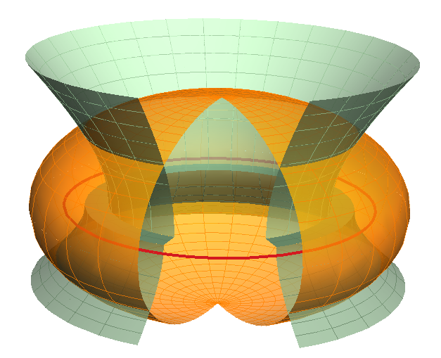
Refer to caption
Figure 2: The real and imaginary parts of ζ=ξ−i​η\zeta=\xi-i\eta, together with the azimuthal angle ϕ\phi, form an oblate spheroidal coordinate system (ξ,η,ϕ)(\xi,\eta,\phi) in ℝ3{{\mathbb{R}}^{3}}. The above plot shows cut-away views of an oblate spheroid 𝒪ξ{\mathcal{O}}_{\xi} with ξ=0.7​a\xi=0.7a, a semi-hyperboloid ℋη{\mathcal{H}}_{\eta} with η=0.8​a​(z>0)\eta=0.8a\,(z>0) and another with η=−0.5​a​(z<0)\eta=-0.5a\,(z<0). Also shown is the focal circle 𝒞{\mathcal{C}} with radius aa at z=0z=0, whose interior is the branch disk 𝒟{\mathcal{D}} of ζ\zeta.

To see that Ψ~​(𝒙,t){\tilde{\Psi}}({\boldsymbol{x}},t) is a pulsed beam propagating in the direction of 𝒂{\boldsymbol{a}}, let g0​(t)g_{0}{(t)} be a pulse peaking around t=0t=0. Then at a fixed observation point 𝒙{\boldsymbol{x}},

g⁡(τ−ζ)=12​π​∫0∞d​ω​e−i​ω​(t−ξ)​e−ω⁡(s−η)​g^0​(ω)\displaystyle g(\tau-\zeta)=\frac{1}{2\pi}\int_{0}^{\infty}{\rm d}\omega\,e^{-i\omega(t-\xi)}e^{-\omega(s-\eta)}{\hat{g}}_{0}{(\omega)} (24)

is a pulse peaking around t=ξ⁡(𝒙)t=\xi({\boldsymbol{x}}). Hence the wavefronts of Ψ~​(𝒙,t){\tilde{\Psi}}({\boldsymbol{x}},t) consist of the oblate spheroids 𝒪ξ{\mathcal{O}}_{\xi}, just as the wavefronts of Ψ⁡(𝒙,t)\Psi({\boldsymbol{x}},t) in (11) are the spheres r=tr=t.

But the pulse amplitude is not uniform on 𝒪ξ{\mathcal{O}}_{\xi}. Due to the factor e−ω⁡(s−η)e^{-\omega(s-\eta)} in (24), it is strongest along the positive zz-axis, where η=a\eta=a, and weakest along the negative zz-axis, where η=−a\eta=-a. In fact, if we follow a propagating wavefront along any given semi-hyperboloid ℋη{\mathcal{H}}_{\eta} (i.e., fix η=η0\eta=\eta_{0} and let ξ\xi increase as ξ⁡(t)=t+ξ0\xi{(t)}=t+\xi_{0}), then

Ψ~​(𝒙,t)=g⁡(−ξ0−i⁡(s−η0))t+ξ0−i​η0∼g⁡(−ξ0−i⁡(s−η0))t,t≫|ξ0−i​η0|.\displaystyle{\tilde{\Psi}}({\boldsymbol{x}},t)=\frac{g(-\xi_{0}-i(s-\eta_{0}))}{t+\xi_{0}-i\eta_{0}}\sim\frac{g(-\xi_{0}-i(s-\eta_{0}))}{t},\quad t\gg|\xi_{0}-i\eta_{0}|.

The numerator remains constant, and the attenuation of Ψ~{\tilde{\Psi}} is due entirely to the increasing distance, i.e., size of the denominator. This shows that Ψ~{\tilde{\Psi}} propagates along ℋη{\mathcal{H}}_{\eta}, so each ℋη{\mathcal{H}}_{\eta} is a diffraction surface for the pulsed beam. In the far zone, 𝒪ξ{\mathcal{O}}_{\xi} becomes a spherical wavefront (ξ≈r\xi\approx r) and ℋη{\mathcal{H}}_{\eta} becomes a diffraction cone (η≈a​cos⁡θ\eta\approx a\cos\theta) for the beam.

In the frequency domain, Ψ~{\tilde{\Psi}} is represented by

Ψ~ω​(𝒙)=g^0​(ω)​ei​k​ζζ=g^0​(ω)​ei​k​ξζ​ek​η,ω>0,\displaystyle{\tilde{\Psi}}_{\omega}({\boldsymbol{x}})={\hat{g}}_{0}{(\omega)}\frac{e^{ik\zeta}}{\zeta}={\hat{g}}_{0}{(\omega)}\frac{e^{ik\xi}}{\zeta}\,e^{k\eta},\quad\omega>0, (25)

where k=ω/c≡ωk=\omega/c\equiv\omega is the wave number and we have suppressed the factor e−ω​se^{-\omega s}, which controls the growth as ω→∞\omega\to\infty. These are the original complex-source beams derived by Deschamps [D71]. In the far zone,

r≫a⇒Ψ~ω​(𝒙)∼g^0​(ω)​ei​k​rr​ek​a​cos⁡θ,\displaystyle r\gg a\ \Rightarrow\ {\tilde{\Psi}}_{\omega}({\boldsymbol{x}})\sim{\hat{g}}_{0}{(\omega)}\frac{e^{ikr}}{r}\,e^{ka\cos\theta},

showing that the radiation pattern of the beam is

ℱω​(θ)=g^0​(ω)​ek​a​cos⁡θ.\displaystyle{\mathcal{F}}_{\omega}{(\theta)}={\hat{g}}_{0}{(\omega)}\,e^{ka\cos\theta}.

Applications of complex-source beams in electrical engineering were developed extensively by Felsen and later extended to the time domain by Heyman et al. using analytic signals. See [F76, HF89]; also [HK9] and references therein.

The spacetime analytic-signal transform, a tool for extending solutions of wave equations (including the Klein-Gordon and Dirac equations in quantum mechanics) to complex spacetime and their interpretation as directed wave packets (relativistic coherent states), was introduced and developed in [K77, K78, K87, K90, K94, K3].

Remark. The analytic signal g⁡(τ)g{(\tau)} can be interpreted as follows. Whereas the point source δ⁡(𝒙)\delta({\boldsymbol{x}}) can be driven by an arbitrary time signal g0​(t)g_{0}{(t)}, the disk 𝒟{\mathcal{D}} must be driven by a separate time signal g0​(𝝆,t)g_{0}({\boldsymbol{\rho}},t) for each 𝝆∈𝒟{\boldsymbol{\rho}}\in{\mathcal{D}}. However, these signals cannot be independent since the points 𝝆{\boldsymbol{\rho}} are rigidly connected to 𝒟{\mathcal{D}}. By the magic of complex analysis, the single analytic function g⁡(t−i​s)g(t-is) represents a coherent driving signal for the entire disk. The imaginary time parameter ss represents a reaction time measuring the degree of correlation. Increasing ss makes g⁡(t−i​s)g(t-is) smoother, hence more correlated. In (24), for example, we must require that

s−η≥0​∀𝒙,hences≥a≡a/c,\displaystyle s-\eta\geq 0\ \forall{\boldsymbol{x}},\ \ \hbox{hence}\ \ s\geq a\equiv a/c,

in order for the integral to converge when gg is a general square-integrable signal. This implies that the correlations between all points on 𝒟{\mathcal{D}} are related causally.

3 The twisted null congruence of Ψ~{\tilde{\Psi}}

We now show that the oblate spheroids 𝒪ξ{\mathcal{O}}_{\xi} and semi-hyperboloids ℋη{\mathcal{H}}_{\eta} can be understood geometrically as the wavefronts and diffraction surfaces, respectively, of ‘light rays’ (points moving in straight lines at speed cc) emitted from the disk 𝒟{\mathcal{D}} if the latter is assumed to spin at the extreme relativistic angular velocity c/ac/a. This will later inspire the construction of coherent electromagnetic wavelets, which fully justify the interpretation in terms of light rays.

We have shown that ℋη{\mathcal{H}}_{\eta} should be interpreted as a diffraction surface for the pulsed beam Ψ~{\tilde{\Psi}}, i.e., a surface along which ζ​Ψ~=g⁡(τ−ζ)\zeta{\tilde{\Psi}}=g(\tau-\zeta) is constant when the wavefront 𝒪ξ{\mathcal{O}}_{\xi} expands as ξ=t\xi=t. We now refine this interpretation.

In Figure 2, imagine that ℋη{\mathcal{H}}_{\eta} consists of individual ‘rays’ propagating away from the source disk in the direction orthogonal to the wavefront 𝒪ξ{\mathcal{O}}_{\xi}. The location of the points tracing out the rays is given in oblate spheroidal coordinates (ξ,η,ϕ)(\xi,\eta,\phi) with

ξ=t,η=η0,ϕ=ϕ0,\displaystyle\xi=t,\quad\eta=\eta_{0},\quad\phi=\phi_{0},

with η0\eta_{0} and ϕ0\phi_{0} fixed. We shall use ξ\xi as the time parameter to describe the motion. The trajectory of the ray in space is then

𝒙0(ξ)=(ρ(ξ)cosϕ0,ρ(ξ)sinϕ0,z(ξ)),\displaystyle{\boldsymbol{x}}_{0}{(\xi)}=(\rho{(\xi)}\cos\phi_{0},\rho{(\xi)}\sin\phi_{0},z{(\xi)}), (26)

and (20) gives

a2​ρ​(ξ)2=(ξ2+a2)​(a2−η02),a​z​(ξ)=ξ​η0.\displaystyle a^{2}\rho{(\xi)}^{2}=(\xi^{2}+a^{2})(a^{2}-\eta_{0}^{2}),\quad az{(\xi)}=\xi\eta_{0}\,.

Its velocity is

𝒗0​(ξ)=∂t𝒙0​(ξ)=(ρξ​cos⁡ϕ,ρξ​sin⁡ϕ,zξ)\displaystyle{\boldsymbol{v}}_{0}{(\xi)}=\partial_{t}{\boldsymbol{x}}_{0}{(\xi)}=(\rho_{\xi}\cos\phi,\rho_{\xi}\sin\phi,z_{\xi})

where

ρξ≡∂ξρ=ξ⁡(a2−η02)a2​ρ,zξ≡∂ξz=η0a.\displaystyle\rho_{\xi}\equiv\partial_{\xi}\rho=\frac{\xi(a^{2}-\eta_{0}^{2})}{a^{2}\rho},\quad z_{\xi}\equiv\partial_{\xi}z=\frac{\eta_{0}}{a}.

It follows that

𝒗02=ρξ2+zξ2=ξ2+η02ξ2+a2.\displaystyle{\boldsymbol{v}}_{0}^{2}=\rho_{\xi}^{2}+z_{\xi}^{2}=\frac{\xi^{2}+\eta_{0}^{2}}{\xi^{2}+a^{2}}\,. (27)

Since ρ​(0)2=a2−η02\rho{(0)}^{2}=a^{2}-\eta_{0}^{2}, the rays starting from the center of the disk (ρ⁡(0)=0\rho{(0)}=0) have η0=±a\eta_{0}=\pm a and travel in straight lines with speed |𝒗0|=1|{\boldsymbol{v}}_{0}|=1. But all other rays, starting with 0<ρ⁡(0)≤a0<\rho{(0)}\leq a, have η02=a2−ρ​(0)2<a2\eta_{0}^{2}=a^{2}-\rho{(0)}^{2}<a^{2}, hence their propagation speed is |𝒗0|<1|{\boldsymbol{v}}_{0}|<1 and their paths are hyperbolic.

Ideally, we would like our ‘rays’ to travel like light in free space: in straight lines, and at speed cc. This can be arranged by allowing ϕ\phi to vary in time. Let the ray have the trajectory

𝒙⁡(ξ)=(ρ⁡(ξ)​cos⁡ϕ⁡(ξ),ρ⁡(ξ)​sin⁡ϕ⁡(ξ),z⁡(ξ)),\displaystyle{\boldsymbol{x}}{(\xi)}=(\rho{(\xi)}\cos\phi{(\xi)},\rho{(\xi)}\sin\phi{(\xi)},z{(\xi)}),

so that its velocity is

𝒗⁡(ξ)≡∂t𝒙⁡(ξ)=𝒗0​(ξ)+ρ⁡(ξ)​ϕ′​(ξ)​ϕ^\displaystyle{\boldsymbol{v}}{(\xi)}\equiv\partial_{t}{\boldsymbol{x}}{(\xi)}={\boldsymbol{v}}_{0}{(\xi)}+\rho{(\xi)}\phi^{\prime}{(\xi)}\mbox{\boldmath{{$\rm\hat{\phi}$}}}

where

ϕ^=∂ϕ𝝆^=∂ϕ(cos⁡ϕ,sin⁡ϕ,0)=(−sin⁡ϕ,cos⁡ϕ,0).\displaystyle\mbox{\boldmath{{$\rm\hat{\phi}$}}}=\partial_{\phi}\mbox{\boldmath{{$\rm\hat{\rho}$}}}=\partial_{\phi}(\cos\phi,\sin\phi,0)=(-\sin\phi,\cos\phi,0).

We require that |𝒗⁡(ξ)|≡1|{\boldsymbol{v}}{(\xi)}|\equiv 1, hence (27) gives

ρ2​ϕ′2=1−ξ2+η02ξ2+a2=a2−η02ξ2+a2⇒ϕ′2=a2(ξ2+a2)2.\displaystyle\rho^{2}\phi^{\prime 2}=1-\frac{\xi^{2}+\eta_{0}^{2}}{\xi^{2}+a^{2}}=\frac{a^{2}-\eta_{0}^{2}}{\xi^{2}+a^{2}}\ \Rightarrow\ \phi^{\prime 2}=\frac{a^{2}}{(\xi^{2}+a^{2})^{2}}.

That is, the points of the circle

𝒞ξ−i​η0=𝒪ξ∩ℋη0\displaystyle{\mathcal{C}}_{\xi-i\eta_{0}}={\mathcal{O}}_{\xi}\cap{\mathcal{H}}_{\eta_{0}}

propagate precisely at the speed c=1c=1 if and only if 𝒞ξ−i​η0{\mathcal{C}}_{\xi-i\eta_{0}} spins at the angular velocity

ω±​(ξ)=ϕ′​(ξ)=±aξ2+a2≡±c​aξ2+a2.\displaystyle\boxed{\ \omega_{\pm}{(\xi)}=\phi^{\prime}{(\xi)}=\pm\frac{a}{\xi^{2}+a^{2}}\equiv\pm\frac{ca}{\xi^{2}+a^{2}}.\ } (28)

Furthermore, since ϕ′​(ξ)\phi^{\prime}{(\xi)} is independent of η0\eta_{0}, all the circles 𝒞ξ−i​η0{\mathcal{C}}_{\xi-i\eta_{0}} with given ξ\xi spin at the same angular velocity and the oblate spheroid 𝒪ξ{\mathcal{O}}_{\xi} spins as a rigid body. We say that the spheroid with angular velocity ω+\omega_{+} has positive helicity and that with angular velocity ω−\omega_{-} has negative helicity.

Since the branch disk 𝒟{\mathcal{D}} is the limit of 𝒪ξ{\mathcal{O}}_{\xi} as ξ→0\xi\to 0, it follows that 𝒟{\mathcal{D}} spins rigidly at ω±(0)=±c/a\omega_{\pm}{(0)}=\pm c/a. This is precisely the angular velocity at which the points on the boundary ∂𝒟\partial{\mathcal{D}} move at the speed of light! More will be said about this in Section 4.

Let us now compute the trajectory of a single point of 𝒞ξ−i​η0{\mathcal{C}}_{\xi-i\eta_{0}}. We can set ϕ0=0\phi_{0}=0 without loss of generality. Integrating (28) gives

ϕ⁡(ξ)=±tan−1⁡(ξ/a),\displaystyle\phi{(\xi)}=\pm\tan^{-1}(\xi/a), (29)

hence

cos⁡ϕ⁡(ξ)=aξ2+a2andsin⁡ϕ⁡(ξ)=±ξξ2+a2.\displaystyle\cos\phi{(\xi)}=\frac{a}{\sqrt{\xi^{2}+a^{2}}}\ \ \hbox{and}\ \ \sin\phi{(\xi)}=\pm\frac{\xi}{\sqrt{\xi^{2}+a^{2}}}.

Furthermore, a​ρ​(ξ)=(ξ2+a2)​(a2−η02)a\rho{(\xi)}=\sqrt{(\xi^{2}+a^{2})(a^{2}-\eta_{0}^{2})}, so

ρ⁡(ξ)​cos⁡ϕ​(ξ)\displaystyle\rho{(\xi)}\cos\phi{(\xi)} =a2−η02=ρ0,ρ⁡(ξ)​sin⁡ϕ⁡(ξ)=±ξ​ρ0a,z⁡(ξ)=t​η0a.\displaystyle=\sqrt{a^{2}-\eta_{0}^{2}}=\rho_{0},\quad\rho{(\xi)}\sin\phi{(\xi)}=\pm\frac{\xi\rho_{0}}{a},\quad z{(\xi)}=\frac{t\eta_{0}}{a}.

The trajectory of the ray starting at the point on 𝒟{\mathcal{D}} with ρ=ρ0\rho=\rho_{0} and ϕ=0\phi=0 is therefore

𝒙⁡(ξ)=(ρ0,±ξ​ρ0a,ξ​η0a)=𝒙⁡(0)+𝒗±​ξ,\displaystyle{\boldsymbol{x}}{(\xi)}=\left(\rho_{0},\pm\frac{\xi\rho_{0}}{a},\frac{\xi\eta_{0}}{a}\right)={\boldsymbol{x}}{(0)}+{\boldsymbol{v}}_{\pm}\xi, (30)

where the velocity is given in Cartesian coordinates by

𝒗±=a−1​(0,±ρ0,η0),𝒗±2=1.\displaystyle{\boldsymbol{v}}_{\pm}=a^{-1}\left(0,\pm\rho_{0},\eta_{0}\right),\quad{\boldsymbol{v}}_{\pm}^{2}=1.

Since the choice ϕ⁡(0)=0\phi{(0)}=0 is arbitrary, we have proved the following result.

Theorem 1

Every point emanating from 𝒟{\mathcal{D}} which follows the exploding wavefront 𝒪ξ{\mathcal{O}}_{\xi} with ξ=c​t\xi=ct as it spins at the angular velocity ω±​(ξ)\omega_{\pm}{(\xi)} while constrained to ℋη0{\mathcal{H}}_{\eta_{0}} moves in a straight line at speed cc.

The trajectories of such points might be interpreted as ‘light rays,’ except that they are associated with a solution of the scalar wave equation rather than Maxwell’s equations. This will be corrected later.

The existence of two families of straight lines generating ℋη{\mathcal{H}}_{\eta} is a well-known fact of geometry: every circular hyperboloid of one sheet is a doubly ruled surface. Our semi-hyperboloids are ruled by the rays, which are half-lines emanating from a circle on 𝒟{\mathcal{D}} as shown in Figure 3. The rays move upwards if η>0\eta>0 and downwards if η<0\eta<0.55 5 In our case, the ruling for η<0\eta<0 has the opposite helicity from that for η>0\eta>0. That is because when the disk spins counterclockwise as seen from the top, it spins clockwise as seen from the bottom. The motion is vertical if η=±a⁡(ρ=0)\eta=\pm a\ (\rho=0). It acquires a horizontal component when 0<|η|<a0<|\eta|<a, and becomes purely horizontal as η→0​(ρ→a)\eta\to 0\ (\rho\to a). For η=0\eta=0, the trajectory begins on the branch circle 𝒞{\mathcal{C}} and is tangent to 𝒞{\mathcal{C}}, remaining in the x​yxy-plane. That is so because 𝒞{\mathcal{C}} is already moving at the speed of light, so the vertical velocity component must vanish. The union of all such horizontal rays forms the degenerate semi-hyperboloid

ℋ0={𝒙:η=0}={𝒙:r≥a,z=0}.\displaystyle{\mathcal{H}}_{0}=\{{\boldsymbol{x}}:\eta=0\}=\{{\boldsymbol{x}}:r\geq a,z=0\}. (31)
Refer to caption
Figure 3: The semi-hyperboloids ℋη{\mathcal{H}}_{\eta} are doubly ruled surfaces, with the straight lines interpreted as ‘light rays’ radiated by 𝒟{\mathcal{D}} and traveling at speed cc.

Let us now compute the velocity vector of the ray going through an arbitrary point 𝒙∈ℝ3{\boldsymbol{x}}\in{{\mathbb{R}}^{3}}. Identifying tt again with ξ\xi, define

𝒖⁡(𝒙)\displaystyle{\boldsymbol{u}}({\boldsymbol{x}}) ≡∂𝒙∂ξ=∂𝒙∂ρ​∂ρ∂ξ+∂𝒙∂z​∂z∂ξ+∂𝒙∂ϕ​∂ϕ∂ξ.\displaystyle\equiv\frac{\partial{\boldsymbol{x}}}{\partial\xi}=\frac{\partial{\boldsymbol{x}}}{\partial\rho}\frac{\partial\rho}{\partial\xi}+\frac{\partial{\boldsymbol{x}}}{\partial z}\frac{\partial z}{\partial\xi}+\frac{\partial{\boldsymbol{x}}}{\partial\phi}\frac{\partial\phi}{\partial\xi}.

Using (20) and

∂𝒙∂ρ=𝝆^\displaystyle\frac{\partial{\boldsymbol{x}}}{\partial\rho}=\mbox{\boldmath{{$\rm\hat{\rho}$}}} ∂𝒙∂z=𝐳^\displaystyle\frac{\partial{\boldsymbol{x}}}{\partial z}=\mbox{\boldmath{{$\rm\hat{z}$}}} ∂𝒙∂ϕ=ρ​ϕ^,\displaystyle\frac{\partial{\boldsymbol{x}}}{\partial\phi}=\rho\mbox{\boldmath{{$\rm\hat{\phi}$}}},

we obtain

𝒖±​(𝒙)=𝝆^​ξa​a2−η2ξ2+a2+𝐳^​ηa±ϕ^​a2−η2ξ2+a2.\displaystyle\boxed{\ {\boldsymbol{u}}_{\pm}({\boldsymbol{x}})=\mbox{\boldmath{{$\rm\hat{\rho}$}}}\,\frac{\xi}{a}\sqrt{\frac{a^{2}-\eta^{2}}{\xi^{2}+a^{2}}}+\mbox{\boldmath{{$\rm\hat{z}$}}}\,\frac{\eta}{a}\pm\mbox{\boldmath{{$\rm\hat{\phi}$}}}\sqrt{\frac{a^{2}-\eta^{2}}{\xi^{2}+a^{2}}}.\ } (32)

In terms of the orthonormal oblate spheroidal basis (𝝃^,𝜼^,ϕ^)(\mbox{\boldmath{{$\rm\hat{\xi}$}}},\mbox{\boldmath{{$\rm\hat{\eta}$}}},\mbox{\boldmath{{$\rm\hat{\phi}$}}}), this is seen to be

𝒖±​(𝒙)=𝝃^​ξ2+η2ξ2+a2±ϕ^​a2−η2ξ2+a2.\displaystyle{\boldsymbol{u}}_{\pm}({\boldsymbol{x}})=\mbox{\boldmath{{$\rm\hat{\xi}$}}}\sqrt{\frac{\xi^{2}+\eta^{2}}{\xi^{2}+a^{2}}}\pm\mbox{\boldmath{{$\rm\hat{\phi}$}}}\sqrt{\frac{a^{2}-\eta^{2}}{\xi^{2}+a^{2}}}. (33)

As expected, the coefficient of 𝜼^\rm\hat{\eta} vanishes since the rays propagate with constant η\eta. Furthermore, 𝒖±{\boldsymbol{u}}_{\pm} is not orthogonal to the wavefront 𝒪ξ{\mathcal{O}}_{\xi} since

𝝃^×𝒖±=±𝜼^​a2−η2ξ2+a2.\displaystyle\mbox{\boldmath{{$\rm\hat{\xi}$}}}\times{\boldsymbol{u}}_{\pm}=\pm\mbox{\boldmath{{$\rm\hat{\eta}$}}}\sqrt{\frac{a^{2}-\eta^{2}}{\xi^{2}+a^{2}}}.

Note that the ϕ\phi-component of 𝒖±{\boldsymbol{u}}_{\pm} does not depend on the sign of η\eta. This confirms that the upper and lower semi-hyperboloids (±η>0\pm\eta>0) are ruled oppositely. Both (32) and (33) show that |𝒖±|=1|{\boldsymbol{u}}_{\pm}|=1, as expected.

The above picture of radiation from a rotating disk explains both the wavefronts 𝒪ξ{\mathcal{O}}_{\xi} and the diffraction surfaces ℋη{\mathcal{H}}_{\eta}. With some poetic license, let us call the emitted particles ‘photons’ even though Ψ~{\tilde{\Psi}} is a scalar potential and not an electromagnetic potential.66 6 In Section 5 we shall reinterpret Ψ~{\tilde{\Psi}} as the scalar component of an electromagnetic 4-vector potential, so that the terminology, while still classical, is not entirely inappropriate. As shown above, the envelope of all the rays emanating from a fixed circle of radius ρ0<a\rho_{0}<a in 𝒟{\mathcal{D}} is the pair of semi-hyperboloids ℋ±η0{\mathcal{H}}_{\pm\eta_{0}} with η0=a2−ρ02\eta_{0}=\sqrt{a^{2}-\rho_{0}^{2}}. However, if we take a snapshot of all the photons at fixed time t=ξ>0t=\xi>0, we find that they form the wavefront 𝒪ξ{\mathcal{O}}_{\xi}. This is illustrated in Figure 4. The radiation from a spinning disk thus explains the level surfaces of both ξ\xi and η\eta, showing the complex distance ζ=ξ−i​η\zeta=\xi-i\eta is a natural tool for its analysis.

Refer to caption
Refer to caption
Figure 4: This picture gives a geometric explanation of ℋη{\mathcal{H}}_{\eta} and 𝒪ξ{\mathcal{O}}_{\xi} in terms of the disk 𝒟{\mathcal{D}} spinning at the extreme relativistic angular velocity c/ac/a. Left: The envelope of the rays emitted from a circle or radius 0<ρ<a0<\rho<a on 𝒟{\mathcal{D}} is the diffraction semi-hyperboloid ℋη{\mathcal{H}}_{\eta} with η=±a2−ρ2\eta=\pm\sqrt{a^{2}-\rho^{2}}. (We show only ℋη{\mathcal{H}}_{\eta} with η=0.7\eta=0.7.) The larger ρ\rho, the greater the horizontal speed and the more twisted is the bundle of rays generating ℋη{\mathcal{H}}_{\eta}. Right: The ‘photons’ emitted from the entire disk 𝒟{\mathcal{D}} at t=0t=0 form the wavefront 𝒪ξ{\mathcal{O}}_{\xi} at t=ξt=\xi.

It can be shown that the vorticity of 𝒖±{\boldsymbol{u}}_{\pm} is given by

𝝎±≡∇×𝒖±=±2​ηξ2+η2​𝒖±.\displaystyle{\boldsymbol{\omega}}_{\pm}\equiv\nabla\times{\boldsymbol{u}}_{\pm}=\pm\frac{2\eta}{\xi^{2}+\eta^{2}}\,{\boldsymbol{u}}_{\pm}. (34)

Thus 𝒖±{\boldsymbol{u}}_{\pm} is a Beltrami field, curling around its own axis with helicity ±\pm.

There is a natural four-dimensional (spacetime) formulation of the above. Consider the two stationary 4-vector fields u±​(𝒙)u_{\pm}({\boldsymbol{x}}) with contravariant and covariant components

u±μ​(𝒙)=(𝒖±​(𝒙),1)uμ±​(𝒙)=(−𝒖±​(𝒙),1),μ=1,2,3,4.\displaystyle u_{\pm}^{\mu}({\boldsymbol{x}})=({\boldsymbol{u}}_{\pm}({\boldsymbol{x}}),1)\quad u^{\pm}_{\mu}({\boldsymbol{x}})=(-{\boldsymbol{u}}_{\pm}({\boldsymbol{x}}),1),\quad\mu=1,2,3,4. (35)

They are null, i.e., their Lorentzian squares with respect to the Minkowski metric ημ​ν=diag⁡(−1,−1,−1,1)\eta_{\mu\nu}={\rm diag}\,(-1,-1,-1,1) vanish:

u±2≡ημ​ν​u±ν​u±μ=uμ±​u±μ=1−𝒖±2=0,\displaystyle u^{2}_{\pm}\equiv\eta_{\mu\nu}u_{\pm}^{\nu}u_{\pm}^{\mu}=u^{\pm}_{\mu}u_{\pm}^{\mu}=1-{\boldsymbol{u}}_{\pm}^{2}=0,

where we sum as usual over the repeated index μ\mu. u±u_{\pm} are the 4-velocities of the twisted ray bundles with helicity ±\pm, and they determine the rays by77 7 Here tt ranges over all real numbers and there is a unique t0t_{0} for which 𝒙+t0​𝒖±∈𝒟{\boldsymbol{x}}+t_{0}{\boldsymbol{u}}_{\pm}\in{\mathcal{D}}. For t>t0t>t_{0}, x±​(𝒙,t)x_{\pm}({\boldsymbol{x}},t) has helicity ±\pm, while for t<t0t<t_{0} it has helicity ∓\mp.

x±μ​(𝒙,t)=(𝒙,0)+t​u±μ​(𝒙)=(𝒙+t​𝒖±​(𝒙),t).\displaystyle x_{\pm}^{\mu}({\boldsymbol{x}},t)=({\boldsymbol{x}},0)+tu_{\pm}^{\mu}({\boldsymbol{x}})=({\boldsymbol{x}}+t{\boldsymbol{u}}_{\pm}({\boldsymbol{x}}),t). (36)

In general relativity, ray bundles (possibly in curved spacetime) such as (36) are called null congruences, and they play an important role in the construction and analysis of nontrivial solutions to the Einstein and Einstein-Maxwell equations; see Section 11. Note that our rays are not orthogonal to the wavefronts 𝒪ξ{\mathcal{O}}_{\xi}. This is a characteristic of twisted congruences, which are characterized by 𝒖⋅∇×𝒖≠0{\boldsymbol{u}}\cdot\nabla\times{\boldsymbol{u}}\neq 0.88 8 In general, a four-dimensional version of (37) must hold. But since 𝒖±{\boldsymbol{u}}_{\pm} depends only on 𝒙{\boldsymbol{x}} and the time component u±0=1u_{\pm}^{0}=1, this reduces to (37). In our case,

𝒖±⋅∇×𝒖±=±2​ηξ2+η2≠0∀z≠0.\displaystyle{\boldsymbol{u}}_{\pm}\cdot\nabla\times{\boldsymbol{u}}_{\pm}=\pm\frac{2\eta}{\xi^{2}+\eta^{2}}\neq 0\quad\forall z\neq 0. (37)

The congruence is twisting everywhere outside the x​yxy-plane, where its rays span the degenerate hyperboloid ℋ0{\mathcal{H}}_{0} (31) of half-lines tangent to 𝒞=∂𝒟{\mathcal{C}}=\partial{\mathcal{D}}.

Remark. It will be shown in Section 11 that the null congruence u±μu^{\mu}_{\pm} in (35) is identical to the null congruences of the Kerr and Kerr-Newman metrics in general relativity [R61, T62, RT64, NJ65, N65]. This is an intriguing fact whose significance remains to be fully understood since the Kerr metric and electromagnetic fields are stationary while Ψ~{\tilde{\Psi}} is time-dependent.

4 Newman’s ‘magic’ electromagnetic field

In 1973, Ted Newman published a paper [N73] detailing the electromagnetic part of the Kerr-Newman solution of the Einstein-Maxwell equations in general relativity [N65], which represents a spinning, charged black hole. Although the Kerr-Newman solution is quite complicated, its purely electromagnetic part is a simple static field in flat spacetime. Newman begins with the analytically continued Coulomb field obtained by replacing the Coulomb potential r−1r^{-1} by ζ−1\zeta^{-1}:

𝐄~​(𝒙)=−∇1ζ=𝒙−i​𝒂ζ3.\displaystyle{\bf{\tilde{E}}}({\boldsymbol{x}})=-\nabla\frac{1}{\zeta}=\frac{{\boldsymbol{x}}-i{\boldsymbol{a}}}{\zeta^{3}}. (38)

He then notes that 𝐄~{\bf{\tilde{E}}} has the following multipole structure:

Re​𝐄~\displaystyle{\,\rm Re}\ {\bf{\tilde{E}}} =(electric monopole)+(electric quadrupole)+⋯\displaystyle=\hbox{(electric monopole)}+\hbox{(electric quadrupole)}+\cdots (39)
Im​𝐄~\displaystyle{\,\rm Im}\ {\bf{\tilde{E}}} =(magnetic dipole)+(magnetic octupole)+⋯.\displaystyle=\hbox{(magnetic dipole)}+\hbox{(magnetic octupole)}+\cdots.

For example, using the far-zone approximation (23) gives

r≫a⇒𝐄~\displaystyle r\gg a\ \Rightarrow\ {\bf{\tilde{E}}} =𝒙−i​𝒂(r−i​𝐱^⋅𝒂)3∼𝒙r3+i​3​𝐱^⋅𝒂−𝒂r3+𝒪⁡(a2/r4).\displaystyle=\frac{{\boldsymbol{x}}-i{\boldsymbol{a}}}{(r-i\mbox{\boldmath{{$\rm\hat{x}$}}}\cdot{\boldsymbol{a}})^{3}}\sim\frac{{\boldsymbol{x}}}{r^{3}}+i\frac{3\mbox{\boldmath{{$\rm\hat{x}$}}}\cdot{\boldsymbol{a}}-{\boldsymbol{a}}}{r^{3}}+{\mathcal{O}}(a^{2}/r^{4}).

The first term is a real electric monopole of charge q=1q=1, and the second term is an imaginary magnetic dipole of magnetic moment 𝒂{\boldsymbol{a}}. Newman therefore interprets 𝐄~{\bf{\tilde{E}}} by writing it as

𝐄~​(𝒙)≡𝑬⁡(𝒙)+i​𝑩​(𝒙),\displaystyle{\bf{\tilde{E}}}({\boldsymbol{x}})\equiv{\boldsymbol{E}}({\boldsymbol{x}})+i{\boldsymbol{B}}({\boldsymbol{x}}), (40)

where 𝑬{\boldsymbol{E}} a real electrostatic field and 𝑩{\boldsymbol{B}} is a real magnetostatic field.

In [K4b], I computed the charge- and current densities of the field (𝑬,𝑩)({\boldsymbol{E}},{\boldsymbol{B}}) as the distributions in ℝ3{{\mathbb{R}}^{3}} defined by

4πϱ(𝒙)=∇⋅𝐄~(𝒙),4π𝑱(𝒙)=−i∇×𝐄~(𝒙)−∂t𝐄~(𝒙)=−i∇×𝐄~(𝒙),\displaystyle 4\pi\varrho({\boldsymbol{x}})=\nabla\cdot{\bf{\tilde{E}}}({\boldsymbol{x}}),\quad 4\pi{\boldsymbol{J}}({\boldsymbol{x}})=-i\nabla\times{\bf{\tilde{E}}}({\boldsymbol{x}})-\partial_{t}{\bf{\tilde{E}}}({\boldsymbol{x}})=-i\nabla\times{\bf{\tilde{E}}}({\boldsymbol{x}}), (41)

which is just the complex form of the usual Maxwell equations. The use of distribution theory is necessary because 𝐄~{\bf{\tilde{E}}} is discontinuous on the branch cut 𝒟{\mathcal{D}} of ζ\zeta and singular on the focal circle 𝒞=∂𝒟{\mathcal{C}}=\partial{\mathcal{D}}, where ζ=0\zeta=0. I showed that:

∙\bullet\ ϱ\varrho and 𝑱{\boldsymbol{J}} are real distributions supported on 𝒟{\mathcal{D}}, so that the homogeneous Maxwell equations are satisfied and thus no magnetic charges or currents are introduced by the complexification.

∙\bullet\ The surface charge-current density on the interior of 𝒟{\mathcal{D}} is given by

σ=−2​a(a2−ρ2)3/2,𝑲=−2​ρ​ϕ^(a2−ρ2)3/2.\displaystyle{\sigma}=-\frac{2a}{(a^{2}-\rho^{2})^{3/2}},\quad{\boldsymbol{K}}=-\frac{2\rho\,\mbox{\boldmath{{$\rm\hat{\phi}$}}}}{(a^{2}-\rho^{2})^{3/2}}. (42)

This is the charge-current density of a rigidly spinning disk rotating in the counterclockwise direction ϕ^\rm\hat{\phi} with angular velocity99 9 The reader may wonder how cc has entered an expression obtained by analytically continuing the Coulomb field. The answer is that the dimensionally correct expression for the current (41) is 4π𝑱(𝒙)=−ic∇×𝐄~(𝒙)−∂t𝐄~(𝒙)=−ic∇×𝐄~(𝒙),\displaystyle 4\pi{\boldsymbol{J}}({\boldsymbol{x}})=-ic\nabla\times{\bf{\tilde{E}}}({\boldsymbol{x}})-\partial_{t}{\bf{\tilde{E}}}({\boldsymbol{x}})=-ic\nabla\times{\bf{\tilde{E}}}({\boldsymbol{x}}), so 𝑲{\boldsymbol{K}} must be multiplied by cc.

ω=|𝑲|σ​ρ=1a≡ca.\displaystyle\omega=\frac{|{\boldsymbol{K}}|}{{\sigma}\rho}=\frac{1}{a}\equiv\frac{c}{a}. (43)

The focal circle 𝒞{\mathcal{C}} therefore spins at the speed of light.1010 10 This bizarre property is related to the fact that 𝐄~{\bf{\tilde{E}}} is the flat-spacetime limit of the electromagnetic field around a spinning charged black hole. That also explains the singular nature of ϱ\varrho and 𝑲{\boldsymbol{K}} on 𝒞{\mathcal{C}}. See [N65, N73]. Note that the speed of a point on 𝒟{\mathcal{D}} is v=c​ρ/av=c\rho/a, hence (42) can be rewritten in a form displaying its relativistic nature:

σ=−2a2​(1−v2/c2)3/2,𝑲=−2​c​ρ​ϕ^a3​(1−v2/c2)3/2.\displaystyle{\sigma}=-\frac{2}{a^{2}(1-v^{2}/c^{2})^{3/2}},\quad{\boldsymbol{K}}=-\frac{2c\rho\,\mbox{\boldmath{{$\rm\hat{\phi}$}}}}{a^{3}(1-v^{2}/c^{2})^{3/2}}. (44)

The surface sources (42) can be obtained easily from the discontinuities of 𝑬{\boldsymbol{E}} and 𝑩{\boldsymbol{B}} across the branch cut 𝒟{\mathcal{D}}. As 𝒙→𝒟{\boldsymbol{x}}\to{\mathcal{D}} from above and below, we have

ρ<a,z→0±⇒ζ→∓i​a2−ρ2,𝒙→ρ​𝝆^≡𝝆.\displaystyle\rho<a,\ z\to 0^{\pm}\ \Rightarrow\ \zeta\to\mp i\sqrt{a^{2}-\rho^{2}},\quad{\boldsymbol{x}}\to\rho\mbox{\boldmath{{$\rm\hat{\rho}$}}}\equiv{\boldsymbol{\rho}}.

The upper and lower boundary values of 𝐄~{\bf{\tilde{E}}} are thus

𝐄~±→𝝆−i​𝒂±i​(a2−ρ2)3/2,\displaystyle{\bf{\tilde{E}}}^{\pm}\to\frac{{\boldsymbol{\rho}}-i{\boldsymbol{a}}}{\pm i(a^{2}-\rho^{2})^{3/2}},

showing that

𝑬±=∓𝒂(a2−ρ2)3/2,𝑩±=∓𝝆(a2−ρ2)3/2,\displaystyle{\boldsymbol{E}}^{\pm}=\mp\frac{{\boldsymbol{a}}}{(a^{2}-\rho^{2})^{3/2}},\quad{\boldsymbol{B}}^{\pm}=\mp\frac{{\boldsymbol{\rho}}}{(a^{2}-\rho^{2})^{3/2}},

and the discontinuities are

δ​𝑬\displaystyle\delta{\boldsymbol{E}} ≡𝑬+−𝑬−=−2​𝒂(a2−ρ2)3/2\displaystyle\equiv{\boldsymbol{E}}^{+}-{\boldsymbol{E}}^{-}=-\frac{2{\boldsymbol{a}}}{(a^{2}-\rho^{2})^{3/2}}
δ​𝑩\displaystyle\delta{\boldsymbol{B}} ≡𝑩+−𝑩−=−2​𝝆(a2−ρ2)3/2.\displaystyle\equiv{\boldsymbol{B}}^{+}-{\boldsymbol{B}}^{-}=-\frac{2{\boldsymbol{\rho}}}{(a^{2}-\rho^{2})^{3/2}}.

The jump conditions at an interface [J99, page 18] thus give

σ\displaystyle{\sigma} =𝐳^⋅δ​𝑬=−2​a(a2−ρ2)3/2\displaystyle=\mbox{\boldmath{{$\rm\hat{z}$}}}\cdot\delta{\boldsymbol{E}}=-\frac{2a}{(a^{2}-\rho^{2})^{3/2}} 𝑲=𝐳^×δ​𝑩=−2​ρ​ϕ^(a2−ρ2)3/2,\displaystyle{\boldsymbol{K}}=\mbox{\boldmath{{$\rm\hat{z}$}}}\times\delta{\boldsymbol{B}}=-\frac{2\rho\,\mbox{\boldmath{{$\rm\hat{\phi}$}}}}{(a^{2}-\rho^{2})^{3/2}}, (45)

proving (42). Furthermore,

𝐳^⋅δ​𝑩=0and𝐳^×δ​𝑬=𝟎,\displaystyle\mbox{\boldmath{{$\rm\hat{z}$}}}\cdot\delta{\boldsymbol{B}}=0\ \ \hbox{and}\ \ \mbox{\boldmath{{$\rm\hat{z}$}}}\times\delta{\boldsymbol{E}}={\boldsymbol{0}}, (46)

proving that the magnetic charge-current density on 𝒟{\mathcal{D}} vanishes as required by the homogeneous Maxwell equations.

However, these surface sources do not give the entire story. The jump conditions do not account for a 1-dimensional charge-current distribution along the boundary 𝒞=∂𝒟{\mathcal{C}}=\partial{\mathcal{D}} since the usual method [J99, page 18] of infinitesimal pillboxes and rectangular line integrals fails there. This failure is reflected by the fact that the total charge of σ{\sigma} is q=−∞q=-\infty, whereas the field 𝐄~{\bf{\tilde{E}}} was derived under the assumption that q=1q=1.

The solution to this puzzle is to compute the complete volume charge-current densities, defined as distributions using (41). When they are computed rigorously (this requires a regularization), we recover (42) on the interior of 𝒟{\mathcal{D}} but also find that ∂𝒟\partial{\mathcal{D}} carries a linear charge-current distribution of charge +∞+\infty, precisely so that the total charge remains q=1q=1.

It is interesting to compute the inertia density ℐ{\mathcal{I}} and energy flow velocity 𝒗{\boldsymbol{v}} of the Newman field 𝐄~{\bf{\tilde{E}}}. By (7),

𝐄~2=1ζ4,henceℐ=12​|ζ4|=12​(ξ2+η2)2,\displaystyle{\bf{\tilde{E}}}^{2}=\frac{1}{\zeta^{4}},\ \ \hbox{hence}\ \ {\mathcal{I}}=\frac{1}{2|\zeta^{4}|}=\frac{1}{2(\xi^{2}+\eta^{2})^{2}}, (47)

which is infinite on the focal circle 𝒞{\mathcal{C}} where ζ=0\zeta=0. Its energy density and Poynting vector are

u\displaystyle u =12​|𝐄~|2=|𝒙−i​𝒂|22​|ζ|4=r2+a22​(ξ2+η2)2=ξ2−η2+2​a22​(ξ2+η2)2\displaystyle=\frac{1}{2}|{\bf{\tilde{E}}}|^{2}=\frac{|{\boldsymbol{x}}-i{\boldsymbol{a}}|^{2}}{2|\zeta|^{4}}=\frac{r^{2}+a^{2}}{2(\xi^{2}+\eta^{2})^{2}}=\frac{\xi^{2}-\eta^{2}+2a^{2}}{2(\xi^{2}+\eta^{2})^{2}} (48)
𝑺\displaystyle{\boldsymbol{S}} =i2​𝐄~×𝐄~∗=𝒂×𝒙|ζ|4=a​ρ(ξ2+η2)2​ϕ^,\displaystyle=\frac{i}{2}{\bf{\tilde{E}}}\times{\bf{\tilde{E}}}^{*}=\frac{{\boldsymbol{a}}\times{\boldsymbol{x}}}{|\zeta|^{4}}=\frac{a\rho}{(\xi^{2}+\eta^{2})^{2}}\,\mbox{\boldmath{{$\rm\hat{\phi}$}}},

so the energy flow velocity is

𝒗=𝑺u=2​a​ρ2​a2+ξ2−η2​ϕ^.\displaystyle{\boldsymbol{v}}=\frac{{\boldsymbol{S}}}{u}=\frac{2a\rho}{2a^{2}+\xi^{2}-\eta^{2}}\mbox{\boldmath{{$\rm\hat{\phi}$}}}. (49)

It follows from (20) with X=a2+ξ2X=a^{2}+\xi^{2} and Y=a2−η2Y=a^{2}-\eta^{2} that

𝒗2\displaystyle{\boldsymbol{v}}^{2} =4​X​Y(X+Y)2=1−(X−Y)2(X+Y)2≤1≡c,\displaystyle=\frac{4XY}{(X+Y)^{2}}=1-\frac{(X-Y)^{2}}{(X+Y)^{2}}\leq 1\equiv c,

with equality only when ξ=η=0\xi=\eta=0, i.e., 𝐱∈𝒞{\boldsymbol{x}}\in{\mathcal{C}}.

Conclusions:

∙\bullet\ Note the similarity between the charge flow (43) on 𝒟{\mathcal{D}} and the twisted congruence derived from Ψ~{\tilde{\Psi}} in Section 3. In both cases, 𝒟{\mathcal{D}} is seen to spin at the extreme relativistic rate ω=c/a\omega=c/a. This will be the inspiration for reinterpreting Ψ~{\tilde{\Psi}} as the scalar part of an electromagnetic 4-potential (𝐀~,Ψ~)({\bf{\tilde{A}}},{\tilde{\Psi}}) whose field is a pulsed version of the Newman field 𝐄~{\bf{\tilde{E}}} (Section 5).

∙\bullet\ The energy field circulates about the zz-axis without propagating out (49), which is expected since the field is non-radiating. Its angular velocity at 𝒙{\boldsymbol{x}} is

Ω⁡(𝒙)=vρ=2​a2​a2+ξ2−η2.\displaystyle\Omega({\boldsymbol{x}})=\frac{v}{\rho}=\frac{2a}{2a^{2}+\xi^{2}-\eta^{2}}. (50)

For fixed ξ>0\xi>0 i.e., 𝐱∈𝒪ξ{\boldsymbol{x}}\in{\mathcal{O}}_{\xi}, Ω⁡(𝒙)\Omega({\boldsymbol{x}}) is a minimum on the equator (η=0)(\eta=0) and increases steadily to its maximum at the north and south poles as |η||\eta| increases from 0 to aa. Hence the energy flow forms a vortex along the zz-axis.

∙\bullet\ On 𝒟⁡(ξ=0){\mathcal{D}}\ (\xi=0), we have

Ω⁡(𝝆)=2​a2​a2−η2=2​aa2+ρ2≡2​a​ca2+ρ2,ρ≤a.\displaystyle\Omega({\boldsymbol{\rho}})=\frac{2a}{2a^{2}-\eta^{2}}=\frac{2a}{a^{2}+\rho^{2}}\equiv\frac{2ac}{a^{2}+\rho^{2}},\quad\rho\leq a.

The angular velocity of the energy flow on 𝒟{\mathcal{D}} differs from the uniform angular velocity ω\omega (43) of the charge flow. It increases from its minimum value Ω⁡(a)=c/a=ω\Omega{(a)}=c/a=\omega on 𝒞{\mathcal{C}} to its maximum value Ω⁡(0)=2​ω\Omega{(0)}=2\omega at the origin, which is the center of the vortex.

∙\bullet\ The real Coulomb field is stationary, as expected:

a→0⇒𝒗→𝟎.\displaystyle a\to 0\ \Rightarrow\ {\boldsymbol{v}}\to{\boldsymbol{0}}.

The rotation thus comes directly from the analytic continuation r→ζr\to\zeta.

5 From scalar to electromagnetic wavelets

In this section we introduce the idea of electromagnetic pulsed-beam wavelets as time-dependent (pulsed) versions of Newman’s static field 𝐄~​(𝒙){\bf{\tilde{E}}}({\boldsymbol{x}}). Like the latter, they will be formulated in complex form as

𝐅~​(𝒙,t)=𝑬⁡(𝒙,t)+i​𝑩​(𝒙,t).\displaystyle{\bf{\tilde{F}}}({\boldsymbol{x}},t)={\boldsymbol{E}}({\boldsymbol{x}},t)+i{\boldsymbol{B}}({\boldsymbol{x}},t). (51)

We begin by interpreting the pulsed beam Ψ~​(𝒙,t){\tilde{\Psi}}({\boldsymbol{x}},t) of Section 2 as a scalar potential and computing a complementary vector potential 𝐀~​(𝒙,t){\bf{\tilde{A}}}({\boldsymbol{x}},t). Both Ψ~{\tilde{\Psi}} and 𝐀~{\bf{\tilde{A}}} are complex. The real field is then obtained as follows. First define the complex fields by complexifying the usual expressions,

𝐄~=−∇Ψ~−∂t𝐀~\displaystyle{\bf{\tilde{E}}}=-\nabla{\tilde{\Psi}}-\partial_{t}{\bf{\tilde{A}}} 𝐁~=∇×𝐀~,\displaystyle{\bf{\tilde{B}}}=\nabla\times{\bf{\tilde{A}}}, (52)

and let

𝐅~=𝐄~+i​𝐁~.\displaystyle{\bf{\tilde{F}}}={\bf{\tilde{E}}}+i{\bf{\tilde{B}}}. (53)

Then (51) implies

𝑬=Re​𝐄~−Im​𝐁~\displaystyle{\boldsymbol{E}}={\,\rm Re}\ {\bf{\tilde{E}}}-{\,\rm Im}\ {\bf{\tilde{B}}} 𝑩=Re​𝐁~+Im​𝐄~.\displaystyle{\boldsymbol{B}}={\,\rm Re}\ {\bf{\tilde{B}}}+{\,\rm Im}\ {\bf{\tilde{E}}}.

Since Ψ~{\tilde{\Psi}} in (12) is retarded, we require that the four-vector (𝐀~,Ψ~)({\bf{\tilde{A}}},{\tilde{\Psi}}) satisfy the Lorenz gauge condition1111 11 Other gauge conditions do not respect causality. While this is acceptable for potentials due to the gauge invariance of the fields, it is not desirable in our case. For example, the fact that Ψ~{\tilde{\Psi}} depends on the complex retarded time τ−ζ\tau-\zeta gave us both the wavefronts 𝒪ξ{\mathcal{O}}_{\xi} and the diffraction semi-hyperboloids ℋη{\mathcal{H}}_{\eta}.

∇⋅𝐀~+∂tΨ~=0.\displaystyle\nabla\cdot{\bf{\tilde{A}}}+\partial_{t}{\tilde{\Psi}}=0. (54)

This relates the unknown vector potential to the known scalar potential. We furthermore require that the current density must vanish outside the branch disk 𝒟{\mathcal{D}} of ζ\zeta, which is also the support of the charge density ϱ~{\tilde{\varrho}} defined in (16):

4​π​𝐉~​(𝒙,t)≡□​𝐀~​(𝒙,t)=𝟎∀𝒙∉𝒟.\displaystyle 4\pi{\bf{\tilde{J}}}({\boldsymbol{x}},t)\equiv\Box{\bf{\tilde{A}}}({\boldsymbol{x}},t)={\boldsymbol{0}}\quad\forall{\boldsymbol{x}}\notin{\mathcal{D}}. (55)

Since we expect 𝐀~{\bf{\tilde{A}}} to have the same time dependence as Ψ~{\tilde{\Psi}}, given by the factor g⁡(τ−ζ)g(\tau-\zeta), we make the Ansatz that

𝐀~​(𝒙,t)=Ψ~​(𝒙,t)​𝒘​(𝒙)\displaystyle\boxed{\ {\bf{\tilde{A}}}({\boldsymbol{x}},t)={\tilde{\Psi}}({\boldsymbol{x}},t){\boldsymbol{w}}({\boldsymbol{x}})\ } (56)

for some static vector field 𝒘⁡(𝒙){\boldsymbol{w}}({\boldsymbol{x}}). This will now be used to solve Equations (54) and (55). Since

∇Ψ~=−g′​(τ−ζ)ζ∇ζ−g⁡(τ−ζ)ζ2∇ζ≡−(g′ζ+gζ2)∇ζ,\displaystyle\nabla{\tilde{\Psi}}=-\frac{g^{\prime}(\tau-\zeta)}{\zeta}\nabla\zeta-\frac{g(\tau-\zeta)}{\zeta^{2}}\nabla\zeta\equiv-\left(\frac{g^{\prime}}{\zeta}+\frac{g}{\zeta^{2}}\right)\nabla\zeta, (57)

we have

∇⋅𝐀~=∇Ψ~⋅𝒘+Ψ~∇⋅𝒘=−(g′ζ+gζ2)∇ζ⋅𝒘+gζ∇⋅𝒘.\displaystyle\nabla\cdot{\bf{\tilde{A}}}=\nabla{\tilde{\Psi}}\cdot{\boldsymbol{w}}+{\tilde{\Psi}}\nabla\cdot{\boldsymbol{w}}=-\left(\frac{g^{\prime}}{\zeta}+\frac{g}{\zeta^{2}}\right)\nabla\zeta\cdot{\boldsymbol{w}}+\frac{g}{\zeta}\nabla\cdot{\boldsymbol{w}}.

Hence (54) requires

−(g′ζ+gζ2)∇ζ⋅𝒘+gζ∇⋅𝒘+g′ζ=0.\displaystyle-\left(\frac{g^{\prime}}{\zeta}+\frac{g}{\zeta^{2}}\right)\nabla\zeta\cdot{\boldsymbol{w}}+\frac{g}{\zeta}\nabla\cdot{\boldsymbol{w}}+\frac{g^{\prime}}{\zeta}=0.

Because this must hold for all analytic signals gg, we have

∇⋅𝐀~+∂tΨ~=0∀g⇔∇ζ⋅𝒘=1and∇⋅𝒘=1ζ.\displaystyle\boxed{\ \nabla\cdot{\bf{\tilde{A}}}+\partial_{t}{\tilde{\Psi}}=0\ \forall g\ \Leftrightarrow\ \nabla\zeta\cdot{\boldsymbol{w}}=1\ \ \hbox{and}\ \ \nabla\cdot{\boldsymbol{w}}=\frac{1}{\zeta}.\ } (58)

Using (56) in (55) gives

□(Ψ~𝒘)=(□Ψ~)𝒘−2(∇Ψ~⋅∇)𝒘−Ψ~Δ𝒘=𝟎∀𝒙∉𝒟.\displaystyle\Box({\tilde{\Psi}}{\boldsymbol{w}})=(\Box{\tilde{\Psi}}){\boldsymbol{w}}-2(\nabla{\tilde{\Psi}}\cdot\nabla){\boldsymbol{w}}-{\tilde{\Psi}}\Delta{\boldsymbol{w}}={\boldsymbol{0}}\ \forall{\boldsymbol{x}}\notin{\mathcal{D}}.

Since □​Ψ~=0\Box{\tilde{\Psi}}=0 outside 𝒟{\mathcal{D}}, the first term vanishes and (57) gives

2(g′ζ+gζ2)(∇ζ⋅∇)𝒘−gζΔ𝒘=𝟎∀𝒙∉𝒟.\displaystyle 2\left(\frac{g^{\prime}}{\zeta}+\frac{g}{\zeta^{2}}\right)(\nabla\zeta\cdot\nabla){\boldsymbol{w}}-\frac{g}{\zeta}\Delta{\boldsymbol{w}}={\boldsymbol{0}}\ \forall{\boldsymbol{x}}\notin{\mathcal{D}}.

Again, this must hold for all gg, hence

(∇ζ⋅∇)𝒘=𝟎andΔ𝒘=𝟎∀𝒙∉𝒟.\displaystyle\boxed{\ (\nabla\zeta\cdot\nabla){\boldsymbol{w}}={\boldsymbol{0}}\ \ \hbox{and}\ \ \Delta{\boldsymbol{w}}={\boldsymbol{0}}\ \forall{\boldsymbol{x}}\notin{\mathcal{D}}.\ } (59)

Finding 𝐀~{\bf{\tilde{A}}} thus reduces to finding a vector field 𝒘⁡(𝒙){\boldsymbol{w}}({\boldsymbol{x}}) satisfying (58) and (59). Amazingly, although this system appears to be overdetermined, we shall find a reasonable set of solutions 𝒘{\boldsymbol{w}}.

Note: If 𝒘=𝒘⁡(𝒙,t){\boldsymbol{w}}={\boldsymbol{w}}({\boldsymbol{x}},t), then (58) remains the same but (59) generalizes to

∂t𝒘+(∇ζ⋅∇)𝒘=𝟎and□𝒘+2ζ∂t𝒘=𝟎.\displaystyle\boxed{\ \partial_{t}{\boldsymbol{w}}+(\nabla\zeta\cdot\nabla){\boldsymbol{w}}={\boldsymbol{0}}\ \ \hbox{and}\ \ \Box{\boldsymbol{w}}+\frac{2}{\zeta}\partial_{t}{\boldsymbol{w}}={\boldsymbol{0}}.\ } (60)

6 The complex spheroidal frame defined by ζ\zeta

Our main tool for computing 𝒘⁡(𝒙){\boldsymbol{w}}({\boldsymbol{x}}) will be a complex moving frame [F63] in ℂ3{{\mathbb{C}\hskip 0.5pt}^{3}} which conforms entirely to the spheroidal geometry defined by ζ\zeta. Let

𝜻^\rm\hat{\zeta} =∇ζ=𝒙−i​𝒂ζ=ρ​𝝆^+z​𝐳^−i​a​𝐳^ζ=ρ​𝝆^+z~​𝐳^ζ,where z~=z−i​a.\displaystyle=\nabla\zeta=\frac{{\boldsymbol{x}}-i{\boldsymbol{a}}}{\zeta}=\frac{\rho\mbox{\boldmath{{$\rm\hat{\rho}$}}}+z\mbox{\boldmath{{$\rm\hat{z}$}}}-ia\mbox{\boldmath{{$\rm\hat{z}$}}}}{\zeta}=\frac{\rho\mbox{\boldmath{{$\rm\hat{\rho}$}}}+{\tilde{z}}\mbox{\boldmath{{$\rm\hat{z}$}}}}{\zeta},\ \ \hbox{where }\ \ {\tilde{z}}=z-ia.

This is the complexification of the real unit vector 𝐫^=∇r\mbox{\boldmath{{$\rm\hat{r}$}}}=\nabla r, and it satisfies

𝜻^2≡𝜻^⋅𝜻^=1.\displaystyle\mbox{\boldmath{{$\rm\hat{\zeta}$}}}^{2}\equiv\mbox{\boldmath{{$\rm\hat{\zeta}$}}}\cdot\mbox{\boldmath{{$\rm\hat{\zeta}$}}}=1.

Note that

(∇ξ−i∇η)2=1⇒|∇ξ|2−|∇η|2=1and∇ξ⋅∇η=0,\displaystyle(\nabla\xi-i\nabla\eta)^{2}=1\ \Rightarrow\ |\nabla\xi|^{2}-|\nabla\eta|^{2}=1\ \ \hbox{and}\ \ \nabla\xi\cdot\nabla\eta=0,

confirming that the levelsurfaces 𝒪ξ{\mathcal{O}}_{\xi} and ℋη{\mathcal{H}}_{\eta} are orthogonal. Define the complexification ϑ\vartheta of the polar angle θ\theta by

sin⁡ϑ=ρζ,cos⁡ϑ=z~ζ,sin2⁡ϑ+cos2⁡ϑ=1,\displaystyle\sin\vartheta=\frac{\rho}{\zeta},\quad\cos\vartheta=\frac{{\tilde{z}}}{\zeta},\quad\sin^{2}\vartheta+\cos^{2}\vartheta=1, (61)

so that

𝜻^=𝝆^​sin⁡ϑ+𝐳^​cos⁡ϑ.\displaystyle\boxed{\ \mbox{\boldmath{{$\rm\hat{\zeta}$}}}=\mbox{\boldmath{{$\rm\hat{\rho}$}}}\sin\vartheta+\mbox{\boldmath{{$\rm\hat{z}$}}}\cos\vartheta.\ } (62)

Next, define the complexification of the unit vector 𝜽^=ϕ^×𝜻^\mbox{\boldmath{{$\rm\hat{\theta}$}}}=\mbox{\boldmath{{$\rm\hat{\phi}$}}}\times\mbox{\boldmath{{$\rm\hat{\zeta}$}}} by

ϑ^=ϕ^×𝜻^=𝝆^​cos⁡ϑ−𝐳^​sin⁡ϑ\displaystyle\boxed{\ \mbox{\boldmath{{$\rm\hat{\vartheta}$}}}=\mbox{\boldmath{{$\rm\hat{\phi}$}}}\times\mbox{\boldmath{{$\rm\hat{\zeta}$}}}=\mbox{\boldmath{{$\rm\hat{\rho}$}}}\cos\vartheta-\mbox{\boldmath{{$\rm\hat{z}$}}}\sin\vartheta\ } (63)

whose real and imaginary parts can be shown to be given by

ϑ^\rm\hat{\vartheta} =ξ​r​𝜽^+a​η​𝝆^ξ2+η2+i​η​r​𝜽^−a​ξ​𝝆^ξ2+η2.\displaystyle=\frac{\xi r\mbox{\boldmath{{$\rm\hat{\theta}$}}}+a\eta\mbox{\boldmath{{$\rm\hat{\rho}$}}}}{\xi^{2}+\eta^{2}}+i\frac{\eta r\mbox{\boldmath{{$\rm\hat{\theta}$}}}-a\xi\mbox{\boldmath{{$\rm\hat{\rho}$}}}}{\xi^{2}+\eta^{2}}.

The three vectors

𝒖1=𝜻^,𝒖2=ϑ^,𝒖3=ϕ^\displaystyle{\boldsymbol{u}}_{1}=\mbox{\boldmath{{$\rm\hat{\zeta}$}}},\quad{\boldsymbol{u}}_{2}=\mbox{\boldmath{{$\rm\hat{\vartheta}$}}},\quad{\boldsymbol{u}}_{3}=\mbox{\boldmath{{$\rm\hat{\phi}$}}} (64)

satisfy the bilinear orthonormality conditions 1212 12 Not the sesquilinear orthonormality condition 𝒖k∗⋅𝒖l=δk​l{\boldsymbol{u}}_{k}^{*}\cdot{\boldsymbol{u}}_{l}=\delta_{kl} based on a hermitian inner product like the one used in quantum mechanics.

𝒖k⋅𝒖l=δk​l\displaystyle{\boldsymbol{u}}_{k}\cdot{\boldsymbol{u}}_{l}=\delta_{kl} (65)

and form a right-handed complex-orthonormal frame in ℂ3{{\mathbb{C}\hskip 0.5pt}^{3}}. Every vector field 𝒘⁡(𝒙){\boldsymbol{w}}({\boldsymbol{x}}) has the unique expansion

𝒘=∑k(𝒘⋅𝒖k)​𝒖k.\displaystyle{\boldsymbol{w}}=\sum_{k}({\boldsymbol{w}}\cdot{\boldsymbol{u}}_{k}){\boldsymbol{u}}_{k}. (66)

The entire basis is determined by the complex distance ζ\zeta, and thus it conforms completely to the associated complex spheroidal geometry. The use of ϕ^\rm\hat{\phi} in defining ϑ^\rm\hat{\vartheta} does not spoil this because ζ\zeta is independent of ϕ\phi. Consequently, the electromagnetic field (51), including its polarization, will conform to this geometry. As we shall see, that makes it possible to construct coherent fields with vanishing inertia because the polarizations on nearby rays do not clash.

Let the unknown vector field 𝒘{\boldsymbol{w}} have the expansion

𝒘⁡(𝒙)=α⁡(𝒙)​𝜻^+β⁡(𝒙)​ϑ^+γ⁡(𝒙)​ϕ^.\displaystyle{\boldsymbol{w}}({\boldsymbol{x}})=\alpha({\boldsymbol{x}})\mbox{\boldmath{{$\rm\hat{\zeta}$}}}+\beta({\boldsymbol{x}})\mbox{\boldmath{{$\rm\hat{\vartheta}$}}}+\gamma({\boldsymbol{x}})\mbox{\boldmath{{$\rm\hat{\phi}$}}}. (67)

We want to use Equations (58) and (59) to compute (α,β,γ)(\alpha,\beta,\gamma). The most difficult one of these would appear to be the first equation in (59), i.e.,

Dζ𝒘=𝟎whereDζ=𝜻^⋅∇,\displaystyle D_{\zeta}{\boldsymbol{w}}={\boldsymbol{0}}\ \ \hbox{where}\ \ D_{\zeta}=\mbox{\boldmath{{$\rm\hat{\zeta}$}}}\cdot\nabla, (68)

since the directional derivative DζD_{\zeta} generally acts on the basis vectors as well as their coefficients. Note that the gradient operator can be expressed by

∇=∇ζ∂ζ+∇ζ∗∂ζ∗+∇ϕ∂ϕ=𝜻^∂ζ+𝜻^∗∂ζ∗+ϕ^ρ∂ϕ\displaystyle\nabla=\nabla\zeta\,\partial_{\zeta}+\nabla\zeta^{*}\partial_{\zeta}^{*}+\nabla\phi\,\partial_{\phi}=\mbox{\boldmath{{$\rm\hat{\zeta}$}}}\partial_{\zeta}+\mbox{\boldmath{{$\rm\hat{\zeta}$}}}^{*}\partial_{\zeta}^{*}+\frac{\mbox{\boldmath{{$\rm\hat{\phi}$}}}}{\rho}\,\partial_{\phi} (69)

where

∂ζ=12(∂ξ+i∂η)\displaystyle\partial_{\zeta}=\frac{1}{2}(\partial_{\xi}+i\partial_{\eta}) ∂ζ∗=12(∂ξ−i∂η)\displaystyle\partial_{\zeta}^{*}=\frac{1}{2}(\partial_{\xi}-i\partial_{\eta}) (70)

are the complex derivatives. Hence (68) becomes

Dζ𝒘=𝟎whereDζ≡𝜻^⋅∇=∂ζ+|𝜻^|2∂ζ∗.\displaystyle\boxed{\ D_{\zeta}{\boldsymbol{w}}={\boldsymbol{0}}\ \ \hbox{where}\ \ D_{\zeta}\equiv\mbox{\boldmath{{$\rm\hat{\zeta}$}}}\cdot\nabla=\partial_{\zeta}+|\mbox{\boldmath{{$\rm\hat{\zeta}$}}}|^{2}\partial_{\zeta}^{*}.\ } (71)

A glimmer of hope appears when we consider the real limit:

𝒂→𝟎⇒Dr→𝐫^⋅∇=∂r.\displaystyle{\boldsymbol{a}}\to{\boldsymbol{0}}\ \Rightarrow\ D_{r}\to\mbox{\boldmath{{$\rm\hat{r}$}}}\cdot\nabla=\partial_{r}.

Since the spherical basis vectors do not depend on rr, we have

∂r𝐫^=∂r𝜽^=∂rϕ^=𝟎,\displaystyle\partial_{r}\mbox{\boldmath{{$\rm\hat{r}$}}}=\partial_{r}\mbox{\boldmath{{$\rm\hat{\theta}$}}}=\partial_{r}\mbox{\boldmath{{$\rm\hat{\phi}$}}}={\boldsymbol{0}}, (72)

and ∂r\partial_{r} does indeed differentiate only the coefficients of a vector field expressed in that basis.

The complex case is more subtle. While the real variables rr and θ\theta are independent, ζ\zeta and ϑ\vartheta cannot be independent as complex variables since they are both functions of (ξ,η)(\xi,\eta).1313 13 The precise relation between ζ\zeta and ϑ\vartheta is 4​a​ζ​sin⁡ϑ\displaystyle 4a\zeta\sin\vartheta =4​a​ρ=4​a2+4​ξ2​4​a2−4​η2=4​a2+(ζ+ζ∗)2​4​a2+(ζ−ζ∗)2.\displaystyle=4a\rho=\sqrt{4a^{2}+4\xi^{2}}\sqrt{4a^{2}-4\eta^{2}}=\sqrt{4a^{2}+(\zeta+\zeta^{*})^{2}}\sqrt{4a^{2}+(\zeta-\zeta^{*})^{2}}. But somewhat miraculously, it turns out that the essential property (72) survives complexification.

Theorem 2

(a) The complexified polar angle ϑ\vartheta is constant with respect to differentiation along the complex direction 𝛇^\rm\hat{\zeta}. That is,

Dζ​ϑ=0.\displaystyle\boxed{\ D_{\zeta}\vartheta=0.\ } (73)

(b) Consequently, the basis vectors {𝛇^,ϑ^,ϕ^}\{\mbox{\boldmath{{$\rm\hat{\zeta}$}}},\mbox{\boldmath{{$\rm\hat{\vartheta}$}}},\mbox{\boldmath{{$\rm\hat{\phi}$}}}\} are are also constant with respect to DζD_{\zeta}:

Dζ​𝜻^=Dζ​ϑ^=Dζ​ϕ^=𝟎.\displaystyle D_{\zeta}\mbox{\boldmath{{$\rm\hat{\zeta}$}}}=D_{\zeta}\mbox{\boldmath{{$\rm\hat{\vartheta}$}}}=D_{\zeta}\mbox{\boldmath{{$\rm\hat{\phi}$}}}={\boldsymbol{0}}. (74)

Proof: (a) Differentiating ζ​sin⁡ϑ=ρ\zeta\sin\vartheta=\rho with respect to ζ∗\zeta^{*} and ζ\zeta gives

ζ​∂ζ∗ϑ​cos⁡ϑ=∂ζ∗ρ\displaystyle\zeta\partial_{\zeta}^{*}\vartheta\cos\vartheta=\partial_{\zeta}^{*}\rho sin⁡ϑ+ζ​∂ζϑ​cos⁡ϑ=∂ζρ\displaystyle\sin\vartheta+\zeta\partial_{\zeta}\vartheta\cos\vartheta=\partial_{\zeta}\rho (75)

From (20) and (70) it follows that

∂ζ∗ρ=−ζ∗​z~2​i​a​ρ=−ζ∗​ζ2​i​a​ρ​cos⁡ϑ\displaystyle\partial_{\zeta}^{*}\rho=-\frac{\zeta^{*}{\tilde{z}}}{2ia\rho}=-\frac{\zeta^{*}\zeta}{2ia\rho}\cos\vartheta ∂ζρ=ζ​z~∗2​i​a​ρ.\displaystyle\partial_{\zeta}\rho=\frac{\zeta{\tilde{z}}^{*}}{2ia\rho}.

The first equation in (75) gives

∂ζ∗ϑ=−ζ∗2​i​a​ρ\displaystyle\partial_{\zeta}^{*}\vartheta=-\frac{\zeta^{*}}{2ia\rho} (76)

and the second equation gives

ζ​∂ζϑ​cos⁡ϑ=ζ​z~∗2​i​a​ρ−ρζ=ζ2​z~∗−2​i​a​ρ22​i​a​ρ​ζ.\displaystyle\zeta\partial_{\zeta}\vartheta\cos\vartheta=\frac{\zeta{\tilde{z}}^{*}}{2ia\rho}-\frac{\rho}{\zeta}=\frac{\zeta^{2}{\tilde{z}}^{*}-2ia\rho^{2}}{2ia\rho\zeta}.

Inserting ζ2=ρ2+z~2\zeta^{2}=\rho^{2}+{\tilde{z}}^{2} and −2​i​a=z~∗−z~-2ia={\tilde{z}}^{*}-{\tilde{z}}, this reduces to

ζ​∂ζϑ​cos⁡ϑ=|z~|2+ρ2ζ∗​ζ⋅ζ∗​z~2​i​a​ρ=|𝜻^|2​ζ∗​z~2​i​a​ρ=|𝜻^|2​ζ∗​ζ2​i​a​ρ​cos⁡ϑ,\displaystyle\zeta\partial_{\zeta}\vartheta\cos\vartheta=\frac{|{\tilde{z}}|^{2}+\rho^{2}}{\zeta^{*}\zeta}\cdot\frac{\zeta^{*}{\tilde{z}}}{2ia\rho}=|\mbox{\boldmath{{$\rm\hat{\zeta}$}}}|^{2}\frac{\zeta^{*}{\tilde{z}}}{2ia\rho}=|\mbox{\boldmath{{$\rm\hat{\zeta}$}}}|^{2}\frac{\zeta^{*}\zeta}{2ia\rho}\cos\vartheta,

which proves that

∂ζϑ=|𝜻^|2ζ∗2​i​a​ρ=−|𝜻^|2∂ζ∗ϑ,henceDζϑ=0.\displaystyle\partial_{\zeta}\vartheta=|\mbox{\boldmath{{$\rm\hat{\zeta}$}}}|^{2}\frac{\zeta^{*}}{2ia\rho}=-|\mbox{\boldmath{{$\rm\hat{\zeta}$}}}|^{2}\partial_{\zeta}^{*}\vartheta,\ \ \hbox{hence}\ \ D_{\zeta}\vartheta=0.

To prove (b), note that

ϑ^=∂ϑ𝜻^\displaystyle\mbox{\boldmath{{$\rm\hat{\vartheta}$}}}=\partial_{\vartheta}\mbox{\boldmath{{$\rm\hat{\zeta}$}}}

by (62) and (63), hence

∂ζ𝜻^=ϑ^​∂ζϑ,∂ζ∗𝜻^=ϑ^​∂ζ∗ϑ\displaystyle\partial_{\zeta}\mbox{\boldmath{{$\rm\hat{\zeta}$}}}=\mbox{\boldmath{{$\rm\hat{\vartheta}$}}}\partial_{\zeta}\vartheta,\quad\partial_{\zeta}^{*}\mbox{\boldmath{{$\rm\hat{\zeta}$}}}=\mbox{\boldmath{{$\rm\hat{\vartheta}$}}}\partial_{\zeta}^{*}\vartheta

and

Dζ​𝜻^=∂ζ𝜻^+|𝜻^|2​∂ζ∗𝜻^=ϑ^​[∂ζϑ+|𝜻^|2​∂ζ∗ϑ]=ϑ^​Dζ​ϑ=𝟎.\displaystyle D_{\zeta}\mbox{\boldmath{{$\rm\hat{\zeta}$}}}=\partial_{\zeta}\mbox{\boldmath{{$\rm\hat{\zeta}$}}}+|\mbox{\boldmath{{$\rm\hat{\zeta}$}}}|^{2}\partial_{\zeta}^{*}\mbox{\boldmath{{$\rm\hat{\zeta}$}}}=\mbox{\boldmath{{$\rm\hat{\vartheta}$}}}\left[\partial_{\zeta}\vartheta+|\mbox{\boldmath{{$\rm\hat{\zeta}$}}}|^{2}\partial_{\zeta}^{*}\vartheta\right]=\mbox{\boldmath{{$\rm\hat{\vartheta}$}}}D_{\zeta}\vartheta={\boldsymbol{0}}. (77)

Furthermore, since ϕ^\rm\hat{\phi} is independent of ζ\zeta and ζ∗\zeta^{*}, we have

Dζ​ϕ^=𝟎andDζ​ϑ^=Dζ​(ϕ^×𝜻^)=ϕ^×Dζ​𝜻^=𝟎.■\displaystyle D_{\zeta}\mbox{\boldmath{{$\rm\hat{\phi}$}}}={\boldsymbol{0}}\ \ \hbox{and}\ \ D_{\zeta}\mbox{\boldmath{{$\rm\hat{\vartheta}$}}}=D_{\zeta}(\mbox{\boldmath{{$\rm\hat{\phi}$}}}\times\mbox{\boldmath{{$\rm\hat{\zeta}$}}})=\mbox{\boldmath{{$\rm\hat{\phi}$}}}\times D_{\zeta}\mbox{\boldmath{{$\rm\hat{\zeta}$}}}={\boldsymbol{0}}.\quad\blacksquare

7 Computing 𝒘⁡(𝒙){\boldsymbol{w}}({\boldsymbol{x}})

We are now ready to compute

𝒘⁡(𝒙)=α⁡(𝒙)​𝜻^+β⁡(𝒙)​ϑ^+γ⁡(𝒙)​ϕ^\displaystyle{\boldsymbol{w}}({\boldsymbol{x}})=\alpha({\boldsymbol{x}})\mbox{\boldmath{{$\rm\hat{\zeta}$}}}+\beta({\boldsymbol{x}})\mbox{\boldmath{{$\rm\hat{\vartheta}$}}}+\gamma({\boldsymbol{x}})\mbox{\boldmath{{$\rm\hat{\phi}$}}} (78)

by enforcing Equations (58) and (59), which are here summarized as

(a)𝜻^⋅𝒘=1,(b)∇⋅𝒘=1ζ,(c)Dζ𝒘=𝟎,(d)Δ𝒘=𝟎.\displaystyle\boxed{\ \hbox{(a)}\ \mbox{\boldmath{{$\rm\hat{\zeta}$}}}\cdot{\boldsymbol{w}}=1,\quad\hbox{(b)}\ \nabla\cdot{\boldsymbol{w}}=\frac{1}{\zeta},\quad\hbox{(c)}\ D_{\zeta}{\boldsymbol{w}}={\boldsymbol{0}},\quad\hbox{(d)}\ \Delta{\boldsymbol{w}}={\boldsymbol{0}}.\ } (79)

∙\bullet\ Equation (79) (a) immediately gives α⁡(𝒙)≡1\alpha({\boldsymbol{x}})\equiv 1.

∙\bullet\ By (71), Dζ​ζ=1,Dζ​ζ∗=|𝜻^|2D_{\zeta}\zeta=1,\,D_{\zeta}\zeta^{*}=|\mbox{\boldmath{{$\rm\hat{\zeta}$}}}|^{2}, and

Dζ​ϑ∗=∂ζϑ∗+|𝜻^|2​∂ζ∗ϑ∗=ζ2​i​a​ρ−|𝜻^|4​ζ2​i​a​ρ≠0.\displaystyle D_{\zeta}\vartheta^{*}=\partial_{\zeta}\vartheta^{*}+|\mbox{\boldmath{{$\rm\hat{\zeta}$}}}|^{2}\partial_{\zeta}^{*}\vartheta^{*}=\frac{\zeta}{2ia\rho}-|\mbox{\boldmath{{$\rm\hat{\zeta}$}}}|^{4}\frac{\zeta}{2ia\rho}\neq 0.

Of the four variables ζ,ζ∗,ϑ,ϑ∗\zeta,\zeta^{*},\vartheta,\vartheta^{*}, only ϑ\vartheta is constant under DζD_{\zeta}. Hence Theorem 2 shows that β\beta and γ\gamma are functions of the angles (ϑ,ϕ)(\vartheta,\phi). That is, they are analytic in ϑ\vartheta, just as Ψ~{\tilde{\Psi}} is analytic in ζ\zeta:

𝒘=𝜻^+β⁡(ϑ,ϕ)​ϑ^+γ⁡(ϑ,ϕ)​ϕ^.\displaystyle{\boldsymbol{w}}=\mbox{\boldmath{{$\rm\hat{\zeta}$}}}+\beta(\vartheta,\phi)\mbox{\boldmath{{$\rm\hat{\vartheta}$}}}+\gamma(\vartheta,\phi)\mbox{\boldmath{{$\rm\hat{\phi}$}}}.

∙\bullet\ Assume that 𝐀~{\bf{\tilde{A}}}, like Ψ~{\tilde{\Psi}}, is axisymmetric, i.e., its components are independent of ϕ\phi. Then

𝒘=𝜻^+β⁡(ϑ)​ϑ^+γ⁡(ϑ)​ϕ^\displaystyle{\boldsymbol{w}}=\mbox{\boldmath{{$\rm\hat{\zeta}$}}}+\beta(\vartheta)\mbox{\boldmath{{$\rm\hat{\vartheta}$}}}+\gamma(\vartheta)\mbox{\boldmath{{$\rm\hat{\phi}$}}} (80)

and

Dζ​𝒘=(Dζ​β)​ϑ^+(Dζ​γ)​ϕ^=β′​(Dζ​ϑ)​ϑ^+γ′​(Dζ​ϑ)​ϕ^=0\displaystyle D_{\zeta}{\boldsymbol{w}}=(D_{\zeta}\beta)\mbox{\boldmath{{$\rm\hat{\vartheta}$}}}+(D_{\zeta}\gamma)\mbox{\boldmath{{$\rm\hat{\phi}$}}}=\beta^{\prime}(D_{\zeta}\vartheta)\mbox{\boldmath{{$\rm\hat{\vartheta}$}}}+\gamma^{\prime}(D_{\zeta}\vartheta)\mbox{\boldmath{{$\rm\hat{\phi}$}}}=0

as required by (79) (c). We now list some relations that will be needed in solving the remaining equations (79) (b) and (d).

Proposition 1
∇ζ=𝜻^\displaystyle\nabla\zeta=\mbox{\boldmath{{$\rm\hat{\zeta}$}}} ∇×𝜻^=𝟎\displaystyle\nabla\times\mbox{\boldmath{{$\rm\hat{\zeta}$}}}={\boldsymbol{0}} ∇⋅𝜻^=2ζ\displaystyle\nabla\cdot\mbox{\boldmath{{$\rm\hat{\zeta}$}}}=\frac{2}{\zeta} Δ​ζ=2ζ\displaystyle\Delta\zeta=\frac{2}{\zeta} Δ​𝜻^=−2​𝜻^ζ2\displaystyle\Delta\mbox{\boldmath{{$\rm\hat{\zeta}$}}}=-\frac{2\mbox{\boldmath{{$\rm\hat{\zeta}$}}}}{\zeta^{2}}
∇ϑ=ϑ^ζ\displaystyle\nabla\vartheta=\frac{\mbox{\boldmath{{$\rm\hat{\vartheta}$}}}}{\zeta} ∇×ϑ^=ϕ^ζ\displaystyle\nabla\times\mbox{\boldmath{{$\rm\hat{\vartheta}$}}}=\frac{\mbox{\boldmath{{$\rm\hat{\phi}$}}}}{\zeta} ∇⋅ϑ^=cos⁡ϑρ\displaystyle\nabla\cdot\mbox{\boldmath{{$\rm\hat{\vartheta}$}}}=\frac{\cos\vartheta}{\rho} Δ​ϑ=cot⁡ϑζ2\displaystyle\Delta\vartheta=\frac{\cot\vartheta}{\zeta^{2}} Δ​ϑ^=−ϑ^+sin⁡2​ϑ​𝜻^ρ2\displaystyle\Delta\mbox{\boldmath{{$\rm\hat{\vartheta}$}}}=-\frac{\mbox{\boldmath{{$\rm\hat{\vartheta}$}}}+\sin 2\vartheta\,\mbox{\boldmath{{$\rm\hat{\zeta}$}}}}{\rho^{2}}
∇ϕ=ϕ^ρ\displaystyle\nabla\phi=\frac{\mbox{\boldmath{{$\rm\hat{\phi}$}}}}{\rho} ∇×ϕ^=𝐳^ρ\displaystyle\nabla\times\mbox{\boldmath{{$\rm\hat{\phi}$}}}=\frac{\mbox{\boldmath{{$\rm\hat{z}$}}}}{\rho} ∇⋅ϕ^=0\displaystyle\nabla\cdot\mbox{\boldmath{{$\rm\hat{\phi}$}}}=0 Δ​ϕ=0\displaystyle\Delta\phi=0 Δ​ϕ^=−ϕ^ρ2.\displaystyle\Delta\mbox{\boldmath{{$\rm\hat{\phi}$}}}=-\frac{\mbox{\boldmath{{$\rm\hat{\phi}$}}}}{\rho^{2}}.

Proofs of the less obvious results are as follows:

∙\displaystyle\bullet\quad ζcosϑ∇ϑ=𝝆^−(𝝆^sinϑ+𝐳^cosϑ)sinϑ=𝝆^cos2ϑ−𝜻^cosϑsinϑ=ϑ^cosϑ\displaystyle\zeta\cos\vartheta\nabla\vartheta=\mbox{\boldmath{{$\rm\hat{\rho}$}}}-(\mbox{\boldmath{{$\rm\hat{\rho}$}}}\sin\vartheta+\mbox{\boldmath{{$\rm\hat{z}$}}}\cos\vartheta)\sin\vartheta=\mbox{\boldmath{{$\rm\hat{\rho}$}}}\cos^{2}\vartheta-\mbox{\boldmath{{$\rm\hat{\zeta}$}}}\cos\vartheta\sin\vartheta=\mbox{\boldmath{{$\rm\hat{\vartheta}$}}}\cos\vartheta
∙\displaystyle\bullet\quad ∇×ϕ^=∇×(ρ∇ϕ)=𝝆^×∇ϕ=𝝆^×ϕ^ρ=𝐳^ρ\displaystyle\nabla\times\mbox{\boldmath{{$\rm\hat{\phi}$}}}=\nabla\times(\rho\nabla\phi)=\mbox{\boldmath{{$\rm\hat{\rho}$}}}\times\nabla\phi=\frac{\mbox{\boldmath{{$\rm\hat{\rho}$}}}\times\mbox{\boldmath{{$\rm\hat{\phi}$}}}}{\rho}=\frac{\mbox{\boldmath{{$\rm\hat{z}$}}}}{\rho}
∙\displaystyle\bullet\quad ∇⋅ϑ^=∇⋅(ϕ^×𝜻^)=𝜻^⋅∇×ϕ^=cos⁡ϑρ\displaystyle\nabla\cdot\mbox{\boldmath{{$\rm\hat{\vartheta}$}}}=\nabla\cdot(\mbox{\boldmath{{$\rm\hat{\phi}$}}}\times\mbox{\boldmath{{$\rm\hat{\zeta}$}}})=\mbox{\boldmath{{$\rm\hat{\zeta}$}}}\cdot\nabla\times\mbox{\boldmath{{$\rm\hat{\phi}$}}}=\frac{\cos\vartheta}{\rho}
∙\displaystyle\bullet\quad ∇⋅ϕ^=∇⋅(ρ∇ϕ)=𝝆^⋅ϕ^+ρΔϕ=0\displaystyle\nabla\cdot\mbox{\boldmath{{$\rm\hat{\phi}$}}}=\nabla\cdot(\rho\nabla\phi)=\mbox{\boldmath{{$\rm\hat{\rho}$}}}\cdot\mbox{\boldmath{{$\rm\hat{\phi}$}}}+\rho\Delta\phi=0
∙\displaystyle\bullet\quad Δ𝜻^=Δ∇ζ=∇Δζ=∇2ζ=−2​𝜻^ζ2.\displaystyle\Delta\mbox{\boldmath{{$\rm\hat{\zeta}$}}}=\Delta\nabla\zeta=\nabla\Delta\zeta=\nabla\frac{2}{\zeta}=-\frac{2\mbox{\boldmath{{$\rm\hat{\zeta}$}}}}{\zeta^{2}}.

Thus

∇⋅𝒘=2ζ+β∇⋅ϑ^+β′∇ϑ⋅ϑ^+γ∇⋅ϕ^+γ′∇ϑ⋅ϕ^=2ζ+β​cos⁡ϑρ+β′ζ\displaystyle\nabla\cdot{\boldsymbol{w}}=\frac{2}{\zeta}+\beta\nabla\cdot\mbox{\boldmath{{$\rm\hat{\vartheta}$}}}+\beta^{\prime}\nabla\vartheta\cdot\mbox{\boldmath{{$\rm\hat{\vartheta}$}}}+\gamma\nabla\cdot\mbox{\boldmath{{$\rm\hat{\phi}$}}}+\gamma^{\prime}\nabla\vartheta\cdot\mbox{\boldmath{{$\rm\hat{\phi}$}}}=\frac{2}{\zeta}+\frac{\beta\cos\vartheta}{\rho}+\frac{\beta^{\prime}}{\zeta}

and Equation (79) (b) becomes

β​cos⁡ϑρ+β′ζ=−1ζ.\displaystyle\frac{\beta\cos\vartheta}{\rho}+\frac{\beta^{\prime}}{\zeta}=-\frac{1}{\zeta}.

To solve this, multiply by ζ​sin⁡ϑ=ρ\zeta\sin\vartheta=\rho:

β​cos⁡ϑ+β′​sin⁡ϑ=∂ϑ(β​sin⁡ϑ)=−sin⁡ϑ,\displaystyle\beta\cos\vartheta+\beta^{\prime}\sin\vartheta=\partial_{\vartheta}(\beta\sin\vartheta)=-\sin\vartheta,

hence

β​sin⁡ϑ=cos⁡ϑ+κ\displaystyle\beta\sin\vartheta=\cos\vartheta+\kappa (81)

where κ\kappa is constant of integration. Thus we have used Equations (79) (a)–(c) to find

𝒘=𝜻^+β​ϑ^+γ​ϕ^whereβ=cot⁡ϑ+κ​csc⁡ϑ.\displaystyle{\boldsymbol{w}}=\mbox{\boldmath{{$\rm\hat{\zeta}$}}}+\beta\mbox{\boldmath{{$\rm\hat{\vartheta}$}}}+\gamma\mbox{\boldmath{{$\rm\hat{\phi}$}}}\ \ \hbox{where}\ \ \beta=\cot\vartheta+\kappa\csc\vartheta. (82)

It remains only to enforce equation (79) (d). We have

Δ​𝒘\displaystyle\Delta{\boldsymbol{w}} =Δ𝜻^+(Δβ)ϑ^+2(∇β⋅∇)ϑ^+βΔϑ^+(Δγ)ϕ^+2(∇γ⋅∇)ϕ^+γΔϕ^\displaystyle=\Delta\mbox{\boldmath{{$\rm\hat{\zeta}$}}}+(\Delta\beta)\mbox{\boldmath{{$\rm\hat{\vartheta}$}}}+2(\nabla\beta\cdot\nabla)\mbox{\boldmath{{$\rm\hat{\vartheta}$}}}+\beta\Delta\mbox{\boldmath{{$\rm\hat{\vartheta}$}}}+(\Delta\gamma)\mbox{\boldmath{{$\rm\hat{\phi}$}}}+2(\nabla\gamma\cdot\nabla)\mbox{\boldmath{{$\rm\hat{\phi}$}}}+\gamma\Delta\mbox{\boldmath{{$\rm\hat{\phi}$}}}
=Δ𝜻^+(Δβ)ϑ^+2β′(∇ϑ⋅∇)ϑ^+βΔϑ^+(Δγ)ϕ^+2γ′(∇ϑ⋅∇)ϕ^+γΔϕ^.\displaystyle=\Delta\mbox{\boldmath{{$\rm\hat{\zeta}$}}}+(\Delta\beta)\mbox{\boldmath{{$\rm\hat{\vartheta}$}}}+2\beta^{\prime}(\nabla\vartheta\cdot\nabla)\mbox{\boldmath{{$\rm\hat{\vartheta}$}}}+\beta\Delta\mbox{\boldmath{{$\rm\hat{\vartheta}$}}}+(\Delta\gamma)\mbox{\boldmath{{$\rm\hat{\phi}$}}}+2\gamma^{\prime}(\nabla\vartheta\cdot\nabla)\mbox{\boldmath{{$\rm\hat{\phi}$}}}+\gamma\Delta\mbox{\boldmath{{$\rm\hat{\phi}$}}}.

We find

β′=−csc2⁡ϑ−κ​cot⁡ϑ​csc⁡ϑ,Δ​β=βρ2,\displaystyle\beta^{\prime}=-\csc^{2}\vartheta-\kappa\cot\vartheta\csc\vartheta,\qquad\Delta\beta=\frac{\beta}{\rho^{2}},
(∇ϑ⋅∇)ϑ^=ϑ^ζ⋅(𝜻^∂ζ+𝜻^∗∂ζ∗+ϕ^ρ∂ϕ)=ϑ^⋅𝜻^∗ζ∂ζ∗ϑ^=−2​i​a​ρζ∗​ζ2∂ζ∗ϑ^.\displaystyle(\nabla\vartheta\cdot\nabla)\mbox{\boldmath{{$\rm\hat{\vartheta}$}}}=\frac{\mbox{\boldmath{{$\rm\hat{\vartheta}$}}}}{\zeta}\cdot\left(\mbox{\boldmath{{$\rm\hat{\zeta}$}}}\partial_{\zeta}+\mbox{\boldmath{{$\rm\hat{\zeta}$}}}^{*}\partial_{\zeta}^{*}+\frac{\mbox{\boldmath{{$\rm\hat{\phi}$}}}}{\rho}\,\partial_{\phi}\right)=\frac{\mbox{\boldmath{{$\rm\hat{\vartheta}$}}}\cdot\mbox{\boldmath{{$\rm\hat{\zeta}$}}}^{*}}{\zeta}\,\partial_{\zeta}^{*}\mbox{\boldmath{{$\rm\hat{\vartheta}$}}}=-\frac{2ia\rho}{\zeta^{*}\zeta^{2}}\,\partial_{\zeta}^{*}\mbox{\boldmath{{$\rm\hat{\vartheta}$}}}.

But

∂ζ∗ϑ^=(∂ζ∗ϑ)​(∂ϑϑ^)=ζ∗2​i​a​ρ​𝜻^,\displaystyle\partial_{\zeta}^{*}\mbox{\boldmath{{$\rm\hat{\vartheta}$}}}=(\partial_{\zeta}^{*}\vartheta)(\partial_{\vartheta}\mbox{\boldmath{{$\rm\hat{\vartheta}$}}})=\frac{\zeta^{*}}{2ia\rho}\mbox{\boldmath{{$\rm\hat{\zeta}$}}},

hence

(∇ϑ⋅∇)ϑ^=−𝜻^ζ2.\displaystyle(\nabla\vartheta\cdot\nabla)\mbox{\boldmath{{$\rm\hat{\vartheta}$}}}=-\frac{\mbox{\boldmath{{$\rm\hat{\zeta}$}}}}{\zeta^{2}}.

Since (∇ϑ⋅∇)ϕ^=𝟎(\nabla\vartheta\cdot\nabla)\mbox{\boldmath{{$\rm\hat{\phi}$}}}={\boldsymbol{0}}, we have

Δ​𝒘\displaystyle\Delta{\boldsymbol{w}} =−2ζ2​𝜻^+βρ2​ϑ^−2​β′ζ2​𝜻^−βρ2​[ϑ^+𝜻^​sin⁡2​ϑ]+[Δ​γ−γρ2]​ϕ^.\displaystyle=-\frac{2}{\zeta^{2}}\mbox{\boldmath{{$\rm\hat{\zeta}$}}}+\frac{\beta}{\rho^{2}}\mbox{\boldmath{{$\rm\hat{\vartheta}$}}}-\frac{2\beta^{\prime}}{\zeta^{2}}\mbox{\boldmath{{$\rm\hat{\zeta}$}}}-\frac{\beta}{\rho^{2}}\left[\mbox{\boldmath{{$\rm\hat{\vartheta}$}}}+\mbox{\boldmath{{$\rm\hat{\zeta}$}}}\sin 2\vartheta\right]+\left[\Delta\gamma-\frac{\gamma}{\rho^{2}}\right]\mbox{\boldmath{{$\rm\hat{\phi}$}}}.

By yet another miracle, the coefficients of 𝛇^\rm\hat{\zeta} and ϑ^\rm\hat{\vartheta} both vanish and we are left with

Δ​𝒘=[Δ​γ−γρ2]​ϕ^.\displaystyle\Delta{\boldsymbol{w}}=\left[\Delta\gamma-\frac{\gamma}{\rho^{2}}\right]\mbox{\boldmath{{$\rm\hat{\phi}$}}}. (83)

Thus (79) (d) requires that γ\gamma satisfy the same equation as β\beta, for which we have already found a general solution:

Δ​𝒘=𝟎⇒Δ​γ=γρ2⇒γ=λ​cot⁡ϑ+μ​csc⁡ϑ.\displaystyle\boxed{\ \Delta{\boldsymbol{w}}={\boldsymbol{0}}\ \Rightarrow\ \Delta\gamma=\frac{\gamma}{\rho^{2}}\ \Rightarrow\ \gamma=\lambda\cot\vartheta+\mu\csc\vartheta.\ } (84)

We have proved the following result.

Theorem 3

The general axisymmetric solution of Equations (79) is

𝒘=𝜻^+(cot⁡ϑ+κ​csc⁡ϑ)​ϑ^+(λ​cot⁡ϑ+μ​csc⁡ϑ)​ϕ^\displaystyle{\boldsymbol{w}}=\mbox{\boldmath{{$\rm\hat{\zeta}$}}}+(\cot\vartheta+\kappa\csc\vartheta)\mbox{\boldmath{{$\rm\hat{\vartheta}$}}}+(\lambda\cot\vartheta+\mu\csc\vartheta)\mbox{\boldmath{{$\rm\hat{\phi}$}}} (85)

where κ,λ,μ\kappa,\lambda,\mu are arbitrary complex constants.

Remark. The solution (85) is singular on the branch disk 𝒟{\mathcal{D}} since ζ\zeta, hence also ϑ\vartheta, is discontinuous there. In fact,

ξ→0,z→0±\displaystyle\xi\to 0,\ z\to 0^{\pm} ⇒ζ→∓i​a2−ρ2,z~→−i​a\displaystyle\ \Rightarrow\ \zeta\to\mp i\sqrt{a^{2}-\rho^{2}},\quad{\tilde{z}}\to-ia
⇒cos⁡ϑ→±aa2−ρ2,sin⁡ϑ→±i​ρa2−ρ2\displaystyle\ \Rightarrow\ \cos\vartheta\to\pm\frac{a}{\sqrt{a^{2}-\rho^{2}}},\quad\sin\vartheta\to\pm i\frac{\rho}{\sqrt{a^{2}-\rho^{2}}}

In addition, 𝒘{\boldsymbol{w}} and thus 𝐀~{\bf{\tilde{A}}}, is singular on the zz-axis. To bring out this singularity, recall that sin⁡ϑ=ρ/ζ\sin\vartheta=\rho/\zeta, hence (85) can be rewritten as

𝒘=𝜻^+ζρ​(cos⁡ϑ+κ)​ϑ^+ζρ​(λ​cos⁡ϑ+μ)​ϕ^.\displaystyle\boxed{\ {\boldsymbol{w}}=\mbox{\boldmath{{$\rm\hat{\zeta}$}}}+\frac{\zeta}{\rho}(\cos\vartheta+\kappa)\mbox{\boldmath{{$\rm\hat{\vartheta}$}}}+\frac{\zeta}{\rho}(\lambda\cos\vartheta+\mu)\mbox{\boldmath{{$\rm\hat{\phi}$}}}.\ } (86)

8 The general pulsed-beam fields 𝐅~±{\bf{\tilde{F}}}_{\pm}

According to (56) and (86), the general axisymmetric vector potential complementing Ψ~{\tilde{\Psi}} is

𝐀~=gζ​𝜻^+gρ​(cos⁡ϑ+κ)​ϑ^+gρ​(λ​cos⁡ϑ+μ)​ϕ^,\displaystyle{\bf{\tilde{A}}}=\frac{g}{\zeta}\mbox{\boldmath{{$\rm\hat{\zeta}$}}}+\frac{g}{\rho}(\cos\vartheta+\kappa)\mbox{\boldmath{{$\rm\hat{\vartheta}$}}}+\frac{g}{\rho}(\lambda\cos\vartheta+\mu)\mbox{\boldmath{{$\rm\hat{\phi}$}}}, (87)

where we have used the shorthand g≡g⁡(τ−ζ)g\equiv g(\tau-\zeta) and κ,λ,μ\kappa,\lambda,\mu are arbitrary complex constants.

Let us compute the complex electric and magnetic fields defined in (53):

𝐄~\displaystyle{\bf{\tilde{E}}} =−∇Ψ~−∂t𝐀~\displaystyle=-\nabla{\tilde{\Psi}}-\partial_{t}{\bf{\tilde{A}}}
=[g′ζ+gζ2]​𝜻^−g′ζ​𝜻^−g′ρ​(cos⁡ϑ+κ)​ϑ^−g′ρ​(λ​cos⁡ϑ+μ)​ϕ^.\displaystyle=\left[\frac{g^{\prime}}{\zeta}+\frac{g}{\zeta^{2}}\right]\mbox{\boldmath{{$\rm\hat{\zeta}$}}}-\frac{g^{\prime}}{\zeta}\mbox{\boldmath{{$\rm\hat{\zeta}$}}}-\frac{g^{\prime}}{\rho}(\cos\vartheta+\kappa)\mbox{\boldmath{{$\rm\hat{\vartheta}$}}}-\frac{g^{\prime}}{\rho}(\lambda\cos\vartheta+\mu)\mbox{\boldmath{{$\rm\hat{\phi}$}}}.

Note that the radiating longitudinal component (g′/ζ)​𝜻^(g^{\prime}/\zeta)\mbox{\boldmath{{$\rm\hat{\zeta}$}}} cancels, leaving only the non-radiating longitudinal component (g/ζ2)​𝜻^(g/\zeta^{2})\mbox{\boldmath{{$\rm\hat{\zeta}$}}}:

𝐄~=gζ2​𝜻^−g′ρ​(cos⁡ϑ+κ)​ϑ^−g′ρ​(λ​cos⁡ϑ+μ)​ϕ^.\displaystyle\boxed{\ {\bf{\tilde{E}}}=\frac{g}{\zeta^{2}}\mbox{\boldmath{{$\rm\hat{\zeta}$}}}-\frac{g^{\prime}}{\rho}(\cos\vartheta+\kappa)\mbox{\boldmath{{$\rm\hat{\vartheta}$}}}-\frac{g^{\prime}}{\rho}(\lambda\cos\vartheta+\mu)\mbox{\boldmath{{$\rm\hat{\phi}$}}}.\ } (88)

The radiation is seen to be confined to the (complex) transversal directions ϑ^\rm\hat{\vartheta} and ϕ^\rm\hat{\phi}. The 1/ρ1/\rho decay of the radiating terms indicates that the singularity along the zz-axis carries a charge-current distribution and thus represents a filament attached to the branch disk. This will be investigated in detail elsewhere.

For computing 𝐁~=∇×𝐀~{\bf{\tilde{B}}}=\nabla\times{\bf{\tilde{A}}}, it will be convenient to rewrite 𝐀~{\bf{\tilde{A}}} as

𝐀~=gζ𝜻^+g(cotϑ+κcscϑ)∇ϑ+g(λcosϑ+μ)∇ϕ,\displaystyle{\bf{\tilde{A}}}=\frac{g}{\zeta}\mbox{\boldmath{{$\rm\hat{\zeta}$}}}+g(\cot\vartheta+\kappa\csc\vartheta)\nabla\vartheta+g(\lambda\cos\vartheta+\mu)\nabla\phi, (89)

where we have used ϑ^=ζ∇ϑ,ϕ^=ρ∇ϕ\mbox{\boldmath{{$\rm\hat{\vartheta}$}}}=\zeta\nabla\vartheta,\,\mbox{\boldmath{{$\rm\hat{\phi}$}}}=\rho\nabla\phi, and ζ/ρ=csc⁡ϑ\zeta/\rho=\csc\vartheta. Then

𝐁~\displaystyle{\bf{\tilde{B}}} =−g′(cotϑ+κcscϑ)𝜻^×∇ϑ−g′(λcosϑ+μ)𝜻^×∇ϕ−λgsinϑ∇ϑ×∇ϕ\displaystyle=-g^{\prime}(\cot\vartheta+\kappa\csc\vartheta)\mbox{\boldmath{{$\rm\hat{\zeta}$}}}\times\nabla\vartheta-g^{\prime}(\lambda\cos\vartheta+\mu)\mbox{\boldmath{{$\rm\hat{\zeta}$}}}\times\nabla\phi-\lambda g\sin\vartheta\nabla\vartheta\times\nabla\phi
=−g′ζ​(cot⁡ϑ+κ​csc⁡ϑ)​ϕ^+g′ρ​(λ​cos⁡ϑ+μ)​ϑ^−λ​g​sin⁡ϑρ​ζ​𝜻^,\displaystyle=-\frac{g^{\prime}}{\zeta}(\cot\vartheta+\kappa\csc\vartheta)\mbox{\boldmath{{$\rm\hat{\phi}$}}}+\frac{g^{\prime}}{\rho}(\lambda\cos\vartheta+\mu)\mbox{\boldmath{{$\rm\hat{\vartheta}$}}}-\frac{\lambda g\sin\vartheta}{\rho\zeta}\mbox{\boldmath{{$\rm\hat{\zeta}$}}},

whose radiative structure is seen more clearly in the form

𝐁~=−λ​gζ2​𝜻^+g′ρ​(λ​cos⁡ϑ+μ)​ϑ^−g′ρ​(cos⁡ϑ+κ)​ϕ^.\displaystyle\boxed{\ {\bf{\tilde{B}}}=-\frac{\lambda g}{\zeta^{2}}\mbox{\boldmath{{$\rm\hat{\zeta}$}}}+\frac{g^{\prime}}{\rho}(\lambda\cos\vartheta+\mu)\mbox{\boldmath{{$\rm\hat{\vartheta}$}}}-\frac{g^{\prime}}{\rho}(\cos\vartheta+\kappa)\mbox{\boldmath{{$\rm\hat{\phi}$}}}.\ } (90)

Note the close similarities between 𝐄~{\bf{\tilde{E}}} and 𝐁~{\bf{\tilde{B}}}, down to the non-radiating longitudinal parts. These similarities combine to give

𝐅~±≡𝐄~±i​𝐁~=p±​gζ2​𝜻^+(q±−p±​cos⁡ϑ)​g′ρ​φ~±\displaystyle\boxed{\ {\bf{\tilde{F}}}_{\pm}\equiv{\bf{\tilde{E}}}\pm i{\bf{\tilde{B}}}=p_{\pm}\frac{g}{\zeta^{2}}\mbox{\boldmath{{$\rm\hat{\zeta}$}}}+(q_{\pm}-p_{\pm}\cos\vartheta)\frac{g^{\prime}}{\rho}{\bf{\tilde{\varphi}}}_{\pm}\ } (91)

where

p±=1∓iλ,q±=−κ±iμ,φ~±=ϑ^±iϕ^.\displaystyle\boxed{\ p_{\pm}=1\mp i\lambda,\quad q_{\pm}=-\kappa\pm i\mu,\quad{\bf{\tilde{\varphi}}}_{\pm}=\mbox{\boldmath{{$\rm\hat{\vartheta}$}}}\pm i\mbox{\boldmath{{$\rm\hat{\phi}$}}}.\ } (92)

Note that φ~+{\bf{\tilde{\varphi}}}_{+} and φ~−{\bf{\tilde{\varphi}}}_{-} are null vectors:

φ~±2=ϑ^2−ϕ^2±2​i​ϑ^⋅ϕ^=0.\displaystyle{\bf{\tilde{\varphi}}}_{\pm}^{2}=\mbox{\boldmath{{$\rm\hat{\vartheta}$}}}^{2}-\mbox{\boldmath{{$\rm\hat{\phi}$}}}^{2}\pm 2i\mbox{\boldmath{{$\rm\hat{\vartheta}$}}}\cdot\mbox{\boldmath{{$\rm\hat{\phi}$}}}=0. (93)

They form a complex basis of helicity ±\pm for the the directions ϑ^,ϕ^\mbox{\boldmath{{$\rm\hat{\vartheta}$}}},\mbox{\boldmath{{$\rm\hat{\phi}$}}} orthogonal to 𝜻^\rm\hat{\zeta}, and will play an important role in the representation of our coherent wavelets. Note also that

φ~±ρ=∇ϑsin⁡ϑ±i∇ϕ=∇ψ±\displaystyle\frac{{\bf{\tilde{\varphi}}}_{\pm}}{\rho}=\frac{\nabla\vartheta}{\sin\vartheta}\pm i\nabla\phi=\nabla\psi_{\pm} (94)

where

ψ±​(ϑ,ϕ)=ln⁡tan⁡(ϑ/2)±i​ϕ=ln⁡(e±i​ϕ​tan⁡(ϑ/2)),\displaystyle\psi_{\pm}(\vartheta,\phi)=\ln\tan(\vartheta/2)\pm i\phi=\ln\left(e^{\pm i\phi}\tan(\vartheta/2)\right), (95)

hence

ρ−1​φ~±⋅d​𝒙=d​ϑsin⁡ϑ±i​d​ϕ=d​ψ±.\displaystyle\boxed{\ \rho^{-1}{\bf{\tilde{\varphi}}}_{\pm}\cdot{\rm d}{\boldsymbol{x}}=\frac{{\rm d}\vartheta}{\sin\vartheta}\pm i{\rm d}\phi={\rm d}\psi_{\pm}.\ } (96)

This can be used to write

𝐅~±⋅d​𝒙=p±​gζ2​d​ζ+(q±−p±​cos⁡ϑ)​g′​d​ψ±.\displaystyle\boxed{\ {\bf{\tilde{F}}}_{\pm}\cdot{\rm d}{\boldsymbol{x}}=p_{\pm}\frac{g}{\zeta^{2}}{\rm d}\zeta+(q_{\pm}-p_{\pm}\cos\vartheta)g^{\prime}{\rm d}\psi_{\pm}.\ } (97)

Remark 1. It might seem that using both complex fields 𝐅~±{\bf{\tilde{F}}}_{\pm} in (91) is superfluous. But since 𝐄~{\bf{\tilde{E}}} and 𝐁~{\bf{\tilde{B}}} are complex, 𝐅~+{\bf{\tilde{F}}}_{+} and 𝐅~−{\bf{\tilde{F}}}_{-} are not related by complex conjugation, thus both fields are needed to recover 𝐄~{\bf{\tilde{E}}} and 𝐁~{\bf{\tilde{B}}}:

2​𝐄~=𝐅~++𝐅~−\displaystyle 2{\bf{\tilde{E}}}={\bf{\tilde{F}}}_{+}+{\bf{\tilde{F}}}_{-} 2​i​𝐁~=𝐅~+−𝐅~−.\displaystyle 2i{\bf{\tilde{B}}}={\bf{\tilde{F}}}_{+}-{\bf{\tilde{F}}}_{-}.

On the other hand, to compute real fields, we need either 𝐅~+{\bf{\tilde{F}}}_{+} or 𝐅~−{\bf{\tilde{F}}}_{-} but not both. Define the two real fields (𝑬+,𝑩+)({\boldsymbol{E}}_{+},{\boldsymbol{B}}_{+}) and (𝑬−,𝑩−)({\boldsymbol{E}}_{-},{\boldsymbol{B}}_{-}) by

𝐅~±=𝑬±±i​𝑩±,\displaystyle{\bf{\tilde{F}}}_{\pm}={\boldsymbol{E}}_{\pm}\pm i{\boldsymbol{B}}_{\pm},

so that

𝑬±\displaystyle{\boldsymbol{E}}_{\pm} =Re​𝐅~±=Re​𝐄~∓Im​𝐁~\displaystyle={\,\rm Re}\ {\bf{\tilde{F}}}_{\pm}={\,\rm Re}\ {\bf{\tilde{E}}}\mp{\,\rm Im}\ {\bf{\tilde{B}}} (98)
𝑩±\displaystyle{\boldsymbol{B}}_{\pm} =±Im​𝐅~±=Re​𝐁~±Im​𝐄~.\displaystyle=\pm{\,\rm Im}\ {\bf{\tilde{F}}}_{\pm}={\,\rm Re}\ {\bf{\tilde{B}}}\pm{\,\rm Im}\ {\bf{\tilde{E}}}\,.

Clearly these two fields are inequivalent, so 𝐅~+{\bf{\tilde{F}}}_{+} and 𝐅~−{\bf{\tilde{F}}}_{-} give two independent real solutions to Maxwell’s equations. Each of these solutions corresponds to a class of equivalent complex fields. Namely, the real field (𝑬±,𝑩±)({\boldsymbol{E}}_{\pm},{\boldsymbol{B}}_{\pm}) remains unchanged when

𝐄~→𝐄~+𝐄~±′and𝐁~→𝐁~+𝐁~±′where𝐁~±′=±i​𝐄~′,\displaystyle{\bf{\tilde{E}}}\to{\bf{\tilde{E}}}+{\bf{\tilde{E}}}^{\prime}_{\pm}\ \ \hbox{and}\ \ {\bf{\tilde{B}}}\to{\bf{\tilde{B}}}+{\bf{\tilde{B}}}^{\prime}_{\pm}\ \ \hbox{where}\ \ {\bf{\tilde{B}}}^{\prime}_{\pm}=\pm i{\bf{\tilde{E}}}^{\prime}, (99)

since this leaves 𝐅~±{\bf{\tilde{F}}}_{\pm} invariant:

𝐅~±→(𝐄~+𝐄~±′)±i⁡(𝐁~±i​𝐄~±′)=𝐄~±i​𝐁~=𝐅~±.\displaystyle{\bf{\tilde{F}}}_{\pm}\to({\bf{\tilde{E}}}+{\bf{\tilde{E}}}^{\prime}_{\pm})\pm i({\bf{\tilde{B}}}\pm i{\bf{\tilde{E}}}^{\prime}_{\pm})={\bf{\tilde{E}}}\pm i{\bf{\tilde{B}}}={\bf{\tilde{F}}}_{\pm}.

If the changes are induced by changes (𝐀~±′,Ψ~±′)({\bf{\tilde{A}}}^{\prime}_{\pm},{\tilde{\Psi}}^{\prime}_{\pm}) of the potentials, then

−∇Ψ~′±−∂t𝐀~′±=𝐄~′±=∓i𝐁~′±=∓i∇×𝐀~′±.\displaystyle-\nabla{\tilde{\Psi}}^{\prime}_{\pm}-\partial_{t}{\bf{\tilde{A}}}^{\prime}_{\pm}={\bf{\tilde{E}}}^{\prime}_{\pm}=\mp i{\bf{\tilde{B}}}^{\prime}_{\pm}=\mp i\nabla\times{\bf{\tilde{A}}}^{\prime}_{\pm}. (100)

Taking the divergence of both sides and using the Lorenz condition gives

−Δ​Ψ~±′−∂t∇⋅𝐀~±′=−Δ​Ψ~±′+∂t2Ψ~±′=□​Ψ~±′=0.\displaystyle-\Delta{\tilde{\Psi}}^{\prime}_{\pm}-\partial_{t}\nabla\cdot{\bf{\tilde{A}}}^{\prime}_{\pm}=-\Delta{\tilde{\Psi}}^{\prime}_{\pm}+\partial_{t}^{2}{\tilde{\Psi}}^{\prime}_{\pm}=\Box{\tilde{\Psi}}^{\prime}_{\pm}=0. (101)

Similarly, taking the curl of (100) yields □​𝐀~±=𝟎\Box{\bf{\tilde{A}}}_{\pm}={\boldsymbol{0}}. The addition of a sourceless term (𝐀~±′,Ψ~±′)({\bf{\tilde{A}}}_{\pm}^{\prime},{\tilde{\Psi}}^{\prime}_{\pm}) to the 4-potential (𝐀~,Ψ~)({\bf{\tilde{A}}},{\tilde{\Psi}}) thus leaves the real field (𝑬±,𝑩±)({\boldsymbol{E}}_{\pm},{\boldsymbol{B}}_{\pm}) invariant. However, this does change the field (𝑬∓,𝑩∓)({\boldsymbol{E}}_{\mp},{\boldsymbol{B}}_{\mp}) of opposite helicity:

𝐅~∓→(𝐄~+𝐄~±′)∓i⁡(𝐁~±i​𝐄~±′)=𝐅~∓+2​𝐄~±′\displaystyle{\bf{\tilde{F}}}_{\mp}\to({\bf{\tilde{E}}}+{\bf{\tilde{E}}}^{\prime}_{\pm})\mp i({\bf{\tilde{B}}}\pm i{\bf{\tilde{E}}}^{\prime}_{\pm})={\bf{\tilde{F}}}_{\mp}+2{\bf{\tilde{E}}}^{\prime}_{\pm}
⇒\displaystyle\ \Rightarrow\ 𝑬∓→𝑬∓+2​Re​𝐄~′,𝑩∓→𝑩∓∓2​Im​𝐄~′.\displaystyle{\boldsymbol{E}}_{\mp}\to{\boldsymbol{E}}_{\mp}+2{\,\rm Re}\ {\bf{\tilde{E}}}^{\prime},\quad{\boldsymbol{B}}_{\mp}\to{\boldsymbol{B}}_{\mp}\mp 2{\,\rm Im}\ {\bf{\tilde{E}}}^{\prime}.

Furthermore, note that (𝑬±,𝑩±)({\boldsymbol{E}}_{\pm},{\boldsymbol{B}}_{\pm}) remains unaffected outside its source region even if (𝐀~±′,Ψ~±′)({\bf{\tilde{A}}}_{\pm}^{\prime},{\tilde{\Psi}}^{\prime}_{\pm}) has a charge-current density whose support is contained in that of (𝐀~,Ψ~)({\bf{\tilde{A}}},{\tilde{\Psi}}). This is a new kind of ‘gauge freedom’ belonging to the complex representation (91). In Secton 11 we shall encounter an example of a ‘pure gauge’ field where 𝐀~≠𝟎{\bf{\tilde{A}}}\neq{\boldsymbol{0}} but 𝐅~±=𝟎{\bf{\tilde{F}}}_{\pm}={\boldsymbol{0}}; see (120).

Remark 2. Equation (91) shows that the radiating parts of the two independent fields (𝑬+,𝑩+)({\boldsymbol{E}}_{+},{\boldsymbol{B}}_{+}) and (𝑬−,𝑩−)({\boldsymbol{E}}_{-},{\boldsymbol{B}}_{-}) associated with 𝐅~+{\bf{\tilde{F}}}_{+} and 𝐅~−{\bf{\tilde{F}}}_{-} have helicity ++ and −-, respectively. This confirms that both fields 𝐅~±{\bf{\tilde{F}}}_{\pm} are needed, as explained above.

9 Coherent electromagnetic wavelets

The inertia density (4) of the field 𝐅~±{\bf{\tilde{F}}}_{\pm} is

ℐ±=12​|𝐅~±2|.\displaystyle{\mathcal{I}}_{\pm}=\frac{1}{2}|{\bf{\tilde{F}}}_{\pm}^{2}|.

Since 𝜻^⋅φ~±=0\mbox{\boldmath{{$\rm\hat{\zeta}$}}}\cdot{\bf{\tilde{\varphi}}}_{\pm}=0 and φ~±2=0{\bf{\tilde{\varphi}}}_{\pm}^{2}=0, (91) gives

𝐅~±2=p±2​g​(τ−ζ)2ζ4.\displaystyle{\bf{\tilde{F}}}_{\pm}^{2}=p_{\pm}^{2}\frac{g(\tau-\zeta)^{2}}{\zeta^{4}}. (102)

Thus one, but not both, of the fields 𝐅~+{\bf{\tilde{F}}}_{+} and 𝐅~−{\bf{\tilde{F}}}_{-} can be made null:

λ=−i\displaystyle\lambda=-i ⇒p+=0⇒𝐅~+=q+​g′​(τ−ζ)ρ​φ~+⇒𝐅~+2=0\displaystyle\ \Rightarrow\ p_{+}=0\ \Rightarrow\ {\bf{\tilde{F}}}_{+}=q_{+}\frac{g^{\prime}(\tau-\zeta)}{\rho}\,{\bf{\tilde{\varphi}}}_{+}\ \Rightarrow\ {\bf{\tilde{F}}}_{+}^{2}=0 (103)
λ=i\displaystyle\lambda=i ⇒p−=0⇒𝐅~−=q−​g′​(τ−ζ)ρ​φ~−⇒𝐅~−2=0.\displaystyle\ \Rightarrow\ p_{-}=0\ \Rightarrow\ {\bf{\tilde{F}}}_{-}=q_{-}\frac{g^{\prime}(\tau-\zeta)}{\rho}\,{\bf{\tilde{\varphi}}}_{-}\ \Rightarrow\ {\bf{\tilde{F}}}_{-}^{2}=0.

Up to a complex scalar factor, we have thus found two unique null fields.

Theorem 4

The field 𝐅~±{\bf{\tilde{F}}}_{\pm} is null if and only if λ=∓i\lambda=\mp i, and then

𝐅~±​(𝒙,t)=g′​(τ−ζ)ρ​φ~±,𝐅~±⋅d​𝒙=g′​(τ−ζ)​d​ψ±\displaystyle\boxed{\ {\bf{\tilde{F}}}_{\pm}({\boldsymbol{x}},t)=\frac{g^{\prime}(\tau-\zeta)}{\rho}\,{\bf{\tilde{\varphi}}}_{\pm},\qquad{\bf{\tilde{F}}}_{\pm}\cdot{\rm d}{\boldsymbol{x}}=g^{\prime}(\tau-\zeta){\rm d}\psi_{\pm}\ } (104)

or a complex scalar multiple thereof, where ψ±\psi_{\pm} is given by (95).

Definition 1

We call 𝐅~±{\bf{\tilde{F}}}_{\pm} the coherent electromagnetic wavelets with helicity ±\pm and driving signal gg.

Recall that 𝐀~{\bf{\tilde{A}}} contained three independent complex parameters κ,λ,μ\kappa,\lambda,\mu. To make 𝐅~±{\bf{\tilde{F}}}_{\pm} null, we must choose λ=∓i\lambda=\mp i, respectively. That leaves two complex parameters, given now by q±q_{\pm} in (103). To reconstruct the complex fields 𝐄~{\bf{\tilde{E}}} and 𝐁~{\bf{\tilde{B}}}, we need both the null field 𝐅~±{\bf{\tilde{F}}}_{\pm} and the non-null field 𝐅~∓{\bf{\tilde{F}}}_{\mp}, hence both q+q_{+} and q−q_{-}. However, if we are interested only in null fields, then we need only q+q_{+} (for positive helicity) or q−q_{-} (for negative helicity).

Theorem 5

𝐅~±{\bf{\tilde{F}}}_{\pm} is an an electromagnetic pulsed beam propagating in the direction of 𝐚{\boldsymbol{a}}, with wavefronts 𝒪ξ{\mathcal{O}}_{\xi} exploding as ξ=c​t\xi=ct, and diffracting along ℋη{\mathcal{H}}_{\eta}.

Proof: Apply the argument used with Equation (24) to interpret Ψ~{\tilde{\Psi}} as a scalar pulsed beam to the pulse-shape factor in (104):

g′(τ−ζ)=−i2​π∫0∞dωωe−i​ω​(t−ξ)e−ω⁡(s−η)g^0(ω).■\displaystyle g^{\prime}(\tau-\zeta)=-\frac{i}{2\pi}\int_{0}^{\infty}{\rm d}\omega\,\omega e^{-i\omega(t-\xi)}e^{-\omega(s-\eta)}{\hat{g}}_{0}{(\omega)}.\quad\blacksquare

Remark. Since φ~±=ϑ^±i​ϕ^{\bf{\tilde{\varphi}}}_{\pm}=\mbox{\boldmath{{$\rm\hat{\vartheta}$}}}\pm i\mbox{\boldmath{{$\rm\hat{\phi}$}}} and

ϑ^=z~​𝝆^−ρ​𝐳^ζ,\displaystyle\mbox{\boldmath{{$\rm\hat{\vartheta}$}}}=\frac{{\tilde{z}}\mbox{\boldmath{{$\rm\hat{\rho}$}}}-\rho\mbox{\boldmath{{$\rm\hat{z}$}}}}{\zeta},

by (63) and (61), 𝐅~±{\bf{\tilde{F}}}_{\pm} is singular on the branch disk 𝒟{\mathcal{D}} of ζ\zeta. Furthermore, (104) shows that it is singular along the zz-axis ρ=0\rho=0. 𝐅~±{\bf{\tilde{F}}}_{\pm} is analytic elsewhere, and this implies that its charge-current distribution is supported on 𝒟{\mathcal{D}}, representing a spinning charged disk, as well as the zz-axis, representing vortex jets generated by the spin of 𝒟{\mathcal{D}} in the positive and negative zz-directions. However, as shown in Theorem 5, the jet along the negative zz-axis is much weaker due to the pulse-shape factor g′​(τ−ζ)g^{\prime}(\tau-\zeta).

The sources of 𝐅~±{\bf{\tilde{F}}}_{\pm} will be studied elsewhere.

10 The real and complex null congruences of 𝐅~±{\bf{\tilde{F}}}_{\pm}

The null fields (103) define both real and complex twisted null congruences in spacetime. The real congruence follow from the nullity condition

(𝑬±±i​𝑩±)2=0⇒𝑺±2≡|𝑬±×𝑩±|2=u±2≡14​(𝑬±2+𝑩±2)2,\displaystyle({\boldsymbol{E}}_{\pm}\pm i{\boldsymbol{B}}_{\pm})^{2}=0\ \Rightarrow\ {\boldsymbol{S}}_{\pm}^{2}\equiv|{\boldsymbol{E}}_{\pm}\times{\boldsymbol{B}}_{\pm}|^{2}=u_{\pm}^{2}\equiv\frac{1}{4}({\boldsymbol{E}}_{\pm}^{2}+{\boldsymbol{B}}_{\pm}^{2})^{2},

which shows that the energy propagates at the speed of light:

𝒗±=𝑺±u±⇒𝒗±2=𝑺±2u±2=1≡c2.\displaystyle{\boldsymbol{v}}_{\pm}=\frac{{\boldsymbol{S}}_{\pm}}{u_{\pm}}\ \Rightarrow\ {\boldsymbol{v}}_{\pm}^{2}=\frac{{\boldsymbol{S}}_{\pm}^{2}}{u_{\pm}^{2}}=1\equiv c^{2}.
Theorem 6

The energy flow velocity for the coherent wavelets (103) is

𝒗±​(𝒙)\displaystyle{\boldsymbol{v}}_{\pm}({\boldsymbol{x}}) =ξa​a2−η2ξ2+a2​𝝆^+ηa​𝐳^±a2−η2ξ2+a2​ϕ^\displaystyle=\frac{\xi}{a}\sqrt{\frac{a^{2}-\eta^{2}}{\xi^{2}+a^{2}}}\,\mbox{\boldmath{{$\rm\hat{\rho}$}}}+\frac{\eta}{a}\,\mbox{\boldmath{{$\rm\hat{z}$}}}\pm\sqrt{\frac{a^{2}-\eta^{2}}{\xi^{2}+a^{2}}}\,\mbox{\boldmath{{$\rm\hat{\phi}$}}} (105)
=𝝃^​ξ2+η2ξ2+a2±ϕ^​a2−η2ξ2+a2,\displaystyle=\mbox{\boldmath{{$\rm\hat{\xi}$}}}\sqrt{\frac{\xi^{2}+\eta^{2}}{\xi^{2}+a^{2}}}\pm\mbox{\boldmath{{$\rm\hat{\phi}$}}}\sqrt{\frac{a^{2}-\eta^{2}}{\xi^{2}+a^{2}}}\,,

which is identical to the velocity field (32)–(33) associated with the scalar wavelet Ψ~{\tilde{\Psi}}. The 4-vector field v±μ=(𝐯±,1)v^{\mu}_{\pm}=({\boldsymbol{v}}_{\pm},1) thus forms a twisting congruence in Minkowski spacetime. This can be expressed as a differential form:

𝒗±​(𝒙)⋅d​𝒙=ξ2+η2ξ2+a2​d​ξ±a2−η2a​d​ϕ.\displaystyle{\boldsymbol{v}}_{\pm}({\boldsymbol{x}})\cdot{\rm d}{\boldsymbol{x}}=\frac{\xi^{2}+\eta^{2}}{\xi^{2}+a^{2}}\,{\rm d}\xi\pm\frac{a^{2}-\eta^{2}}{a}\,{\rm d}\phi. (106)

Proof: Recall from (62) and (63) that

ζ​𝜻^=ρ​𝝆^+z~​𝐳^\displaystyle\zeta\mbox{\boldmath{{$\rm\hat{\zeta}$}}}=\rho\mbox{\boldmath{{$\rm\hat{\rho}$}}}+{\tilde{z}}\mbox{\boldmath{{$\rm\hat{z}$}}} ζ​ϑ^=z~​𝝆^−ρ​𝐳^\displaystyle\zeta\mbox{\boldmath{{$\rm\hat{\vartheta}$}}}={\tilde{z}}\mbox{\boldmath{{$\rm\hat{\rho}$}}}-\rho\mbox{\boldmath{{$\rm\hat{z}$}}} z~=z−i​a.\displaystyle{\tilde{z}}=z-ia.

It follows that

|ζ|2​ϑ^∗⋅ϑ^=r2+a2=|ζ|2​|𝜻^|2=ξ2−η2+2​a2\displaystyle|\zeta|^{2}\mbox{\boldmath{{$\rm\hat{\vartheta}$}}}^{*}\cdot\mbox{\boldmath{{$\rm\hat{\vartheta}$}}}=r^{2}+a^{2}=|\zeta|^{2}|\mbox{\boldmath{{$\rm\hat{\zeta}$}}}|^{2}=\xi^{2}-\eta^{2}+2a^{2}
|ζ|2​ϑ^∗×ϑ^=2​i​a​ρ​ϕ^.\displaystyle|\zeta|^{2}\mbox{\boldmath{{$\rm\hat{\vartheta}$}}}^{*}\times\mbox{\boldmath{{$\rm\hat{\vartheta}$}}}=2ia\rho\mbox{\boldmath{{$\rm\hat{\phi}$}}}.

To simplify the notation, let

X=ξ2+a2andY=a2−η2\displaystyle X=\xi^{2}+a^{2}\ \ \hbox{and}\ \ Y=a^{2}-\eta^{2}

so that

X​Y=a2​ρ2\displaystyle XY=a^{2}\rho^{2} X+Y=ξ2−η2+2​a2\displaystyle X+Y=\xi^{2}-\eta^{2}+2a^{2} X−Y=ξ2+η2=|ζ|2.\displaystyle X-Y=\xi^{2}+\eta^{2}=|\zeta|^{2}.

From φ~±=ϑ^±i​ϕ^{\bf{\tilde{\varphi}}}_{\pm}=\mbox{\boldmath{{$\rm\hat{\vartheta}$}}}\pm i\mbox{\boldmath{{$\rm\hat{\phi}$}}} it follows that

|ζ|2​φ~±∗⋅φ~±=2​X\displaystyle|\zeta|^{2}{\bf{\tilde{\varphi}}}_{\pm}^{*}\cdot{\bf{\tilde{\varphi}}}_{\pm}=2X
|ζ|2​φ~±∗×φ~±=±2​i​[ξ​ρ​𝝆^+(X​η/a)​𝐳^±a​ρ​ϕ^].\displaystyle|\zeta|^{2}{\bf{\tilde{\varphi}}}_{\pm}^{*}\times{\bf{\tilde{\varphi}}}_{\pm}=\pm 2i\left[\xi\rho\mbox{\boldmath{{$\rm\hat{\rho}$}}}+(X\eta/a)\mbox{\boldmath{{$\rm\hat{z}$}}}\pm a\rho\mbox{\boldmath{{$\rm\hat{\phi}$}}}\right].

For the null field 𝐅~±=(g′/ρ)​φ~±{\bf{\tilde{F}}}_{\pm}=(g^{\prime}/\rho){\bf{\tilde{\varphi}}}_{\pm} we have

u±\displaystyle u_{\pm} =12​𝐅~±∗⋅𝐅~±=|g′|2ρ2​2​XX−Y\displaystyle=\frac{1}{2}{\bf{\tilde{F}}}_{\pm}^{*}\cdot{\bf{\tilde{F}}}_{\pm}=\frac{|g^{\prime}|^{2}}{\rho^{2}}\,\frac{2X}{X-Y}
𝑺±\displaystyle{\boldsymbol{S}}_{\pm} =±𝐅~±∗×𝐅~±2​i=|g′|2ρ2​ξ​ρ​𝝆^+(X​η/a)​𝐳^±a​ρ​ϕ^X−Y,\displaystyle=\pm\frac{{\bf{\tilde{F}}}_{\pm}^{*}\times{\bf{\tilde{F}}}_{\pm}}{2i}=\frac{|g^{\prime}|^{2}}{\rho^{2}}\,\frac{\xi\rho\mbox{\boldmath{{$\rm\hat{\rho}$}}}+(X\eta/a)\mbox{\boldmath{{$\rm\hat{z}$}}}\pm a\rho\mbox{\boldmath{{$\rm\hat{\phi}$}}}}{X-Y},

hence

𝒗±​(𝒙)=ξ​ρX​𝝆^+ηa​𝐳^±a​ρX​ϕ^⇒𝒗±2=1.\displaystyle{\boldsymbol{v}}_{\pm}({\boldsymbol{x}})=\frac{\xi\rho}{X}\,\mbox{\boldmath{{$\rm\hat{\rho}$}}}+\frac{\eta}{a}\,\mbox{\boldmath{{$\rm\hat{z}$}}}\pm\frac{a\rho}{X}\,\mbox{\boldmath{{$\rm\hat{\phi}$}}}\ \Rightarrow\ {\boldsymbol{v}}_{\pm}^{2}=1.

Using a​ρ=X​Ya\rho=\sqrt{XY}, we obtain (105). To derive (106), use the identities

|∇ξ|=ξ2+η2ξ2+a2,ϕ^=ρ∇ϕ=(ξ2+a2)​(a2−η2)a∇ϕ.■\displaystyle|\nabla\xi|=\sqrt{\frac{\xi^{2}+\eta^{2}}{\xi^{2}+a^{2}}},\quad\mbox{\boldmath{{$\rm\hat{\phi}$}}}=\rho\nabla\phi=\frac{\sqrt{(\xi^{2}+a^{2})(a^{2}-\eta^{2})}}{a}\nabla\phi.\quad\blacksquare

Note that 𝒗±{\boldsymbol{v}}_{\pm} is time-independent because the pulse factors |g′|2|g^{\prime}|^{2} in 𝑺±{\boldsymbol{S}}_{\pm} and u±u_{\pm} cancel. Therefore the integral curves of 𝒗±{\boldsymbol{v}}_{\pm} are straight lines in ℝ3{{\mathbb{R}}^{3}} propagating at the speed of light. Accompanied by their fields (𝑬±,𝑩±)({\boldsymbol{E}}_{\pm},{\boldsymbol{B}}_{\pm}), these can now be justifiably interpreted as light rays.

Whereas the physical interpretation of the null congruence associated with the scalar wavelet Ψ~{\tilde{\Psi}} was vague because scalar (longitudinal) waves would seem to propagate in the direction orthogonal to their wavefronts, so their congruence could not be twisted, the identical null congruence defined by 𝒗±{\boldsymbol{v}}_{\pm} has a clear physical interpretation: the spinning disk 𝒟{\mathcal{D}} emits light rays whose trajectories are given by

𝒙±​(ξ)=𝝆0+t​𝒗±o,𝝆0∈𝒟,t≥0\displaystyle{\boldsymbol{x}}_{\pm}{(\xi)}={\boldsymbol{\rho}}_{0}+t{\boldsymbol{v}}^{o}_{\pm},\quad{\boldsymbol{\rho}}_{0}\in{\mathcal{D}},\quad t\geq 0
where𝒗±o=Sgn​z​a2−ρ02a​𝐳^±ρ0a​ϕ^.\displaystyle\hbox{where}\ \ {\boldsymbol{v}}^{o}_{\pm}={\,\rm Sgn\,}z\frac{\sqrt{a^{2}-\rho_{0}^{2}}}{a}\,\mbox{\boldmath{{$\rm\hat{z}$}}}\pm\frac{\rho_{0}}{a}\,\mbox{\boldmath{{$\rm\hat{\phi}$}}}.

The rays with ρ0=0\rho_{0}=0 form vertical vortex jets along the zz-axis, while the rays emanating from any circle of radius 0<ρ0<a0<\rho_{0}<a generate the hyperboloid ℋη0∪ℋ−η0{\mathcal{H}}_{\eta_{0}}\cup{\mathcal{H}}_{-\eta_{0}}, with opposite rulings on the upper and lower halves. The rays coming from the circle ρ0=a\rho_{0}=a are tangent to that circle, forming the degenerate hyperboloid ℋ0{\mathcal{H}}_{0}.

To find the complex congruence of 𝐅~±{\bf{\tilde{F}}}_{\pm}, define the complex electromagnetic energy and momentum densities

u~=12​(𝐄~2+𝐁~2),𝐒~=𝐄~×𝐁~.\displaystyle{\tilde{u}}=\frac{1}{2}({\bf{\tilde{E}}}^{2}+{\bf{\tilde{B}}}^{2}),\quad{\bf{\tilde{S}}}={\bf{\tilde{E}}}\times{\bf{\tilde{B}}}. (107)

Letting

L=cos⁡ϑ+κ,M=λ​cos⁡ϑ+μ\displaystyle L=\cos\vartheta+\kappa,\quad M=\lambda\cos\vartheta+\mu

in (88) and (90), we obtain

u~\displaystyle{\tilde{u}} =1+λ22​g2ζ4+g′2ρ2​(L2+M2)\displaystyle=\frac{1+\lambda^{2}}{2}\,\frac{g^{2}}{\zeta^{4}}+\frac{g^{\prime 2}}{\rho^{2}}(L^{2}+M^{2}) (108)
𝐒~\displaystyle{\bf{\tilde{S}}} =g′2ρ2​(L2+M2)​𝜻^+g​g′ζ2​ρ​(L+λ​M)​ϑ^+g​g′ζ2​ρ​(M−λ​L)​ϕ^.\displaystyle=\frac{g^{\prime 2}}{\rho^{2}}(L^{2}+M^{2})\mbox{\boldmath{{$\rm\hat{\zeta}$}}}+\frac{gg^{\prime}}{\zeta^{2}\rho}(L+\lambda M)\mbox{\boldmath{{$\rm\hat{\vartheta}$}}}+\frac{gg^{\prime}}{\zeta^{2}\rho}(M-\lambda L)\mbox{\boldmath{{$\rm\hat{\phi}$}}}.

Now assume that 𝐅~±{\bf{\tilde{F}}}_{\pm} is null. Then λ=∓i\lambda=\mp i and

L2+M2=κ2+μ2=q+​q−,L+λ​M=−q±,M−λ​L=±i​q±,\displaystyle L^{2}+M^{2}=\kappa^{2}+\mu^{2}=q_{+}q_{-},\ L+\lambda M=-q_{\pm},\ M-\lambda L=\pm iq_{\pm},

so

u~\displaystyle{\tilde{u}} =q+​q−​g′2ρ2,𝐒~=q+​q−​g′2ρ2​𝜻^−q±​g​g′ζ2​ρ​φ~±.\displaystyle=q_{+}q_{-}\frac{g^{\prime 2}}{\rho^{2}},\quad{\bf{\tilde{S}}}=q_{+}q_{-}\frac{g^{\prime 2}}{\rho^{2}}\mbox{\boldmath{{$\rm\hat{\zeta}$}}}-q_{\pm}\frac{gg^{\prime}}{\zeta^{2}\rho}\,{\bf{\tilde{\varphi}}}_{\pm}. (109)

Hence the complex energy propagation velocity is

𝐯~±≡𝐒~u~=𝜻^−q∓−1​g​ρg′​ζ2​φ~±.\displaystyle\boxed{\ {\bf{\tilde{v}}}_{\pm}\equiv\frac{{\bf{\tilde{S}}}}{{\tilde{u}}}=\mbox{\boldmath{{$\rm\hat{\zeta}$}}}-q_{\mp}^{-1}\frac{g\rho}{g^{\prime}\zeta^{2}}\,{\bf{\tilde{\varphi}}}_{\pm}\,.\ } (110)

We shall suppress the helicity index ±\pm and write 𝐯~{\bf{\tilde{v}}} for notational simplicity. Thus

𝐯~2=𝜻^2=1≡c2,\displaystyle{\bf{\tilde{v}}}^{2}=\mbox{\boldmath{{$\rm\hat{\zeta}$}}}^{2}=1\equiv c^{2},

so the corresponding complex energy flow velocity 4-vector

v~μ=(𝐯~,1),vμ=(−𝐯~,1)\displaystyle{\tilde{v}}^{\mu}=({\bf{\tilde{v}}},1),\quad v_{\mu}=(-{\bf{\tilde{v}}},1)

defines a null congruence in ℂ4{{\mathbb{C}\hskip 0.5pt}^{4}}:

vμ​vμ=0.\displaystyle v_{\mu}v^{\mu}=0. (111)

To show that this congruence is twisted, consider the complex 1-form

v~\displaystyle{\tilde{v}} ≡v~μ​d​xμ=d​t−𝐯~⋅d​𝒙=d​t−d​ζ+q∓−1​g​ρ2g′​ζ2​d​ψ±,\displaystyle\equiv{\tilde{v}}_{\mu}{\rm d}x^{\mu}={\rm d}t-{\bf{\tilde{v}}}\cdot{\rm d}{\boldsymbol{x}}={\rm d}t-{\rm d}\zeta+q_{\mp}^{-1}\frac{g\rho^{2}}{g^{\prime}\zeta^{2}}\,{\rm d}\psi_{\pm}, (112)

where we have used (96). Since τ=t−i​s\tau=t-is and ss is fixed,

d​t−d​ζ=d​τζwhereτζ=τ−ζ\displaystyle{\rm d}t-{\rm d}\zeta={\rm d}\tau_{\zeta}\ \ \hbox{where}\ \ \tau_{\zeta}=\tau-\zeta (113)

is the complex retarded time. Letting

h⁡(τζ)=q∓−1​g⁡(τζ)g′​(τζ)\displaystyle h(\tau_{\zeta})=q_{\mp}^{-1}\frac{g(\tau_{\zeta})}{g^{\prime}(\tau_{\zeta})}

and recalling that ρ/ζ=sin⁡ϑ\rho/\zeta=\sin\vartheta, we have

v~=d​τζ+h​sin⁡ϑ​d​ϑ±i​h​sin2⁡ϑ​d​ϕ.\displaystyle\boxed{\ {\tilde{v}}={\rm d}\tau_{\zeta}+h\sin\vartheta\,{\rm d}\vartheta\pm ih\sin^{2}\vartheta\,{\rm d}\phi.\ } (114)

The exterior derivative [F63] of v~{\tilde{v}} is given by

d​v~\displaystyle{\rm d}{\tilde{v}} =sin⁡ϑ​d​h∧d​ϑ±i​sin2⁡ϑ​d​h∧d​ϕ±i​h​sin⁡(2​ϑ)​d​ϑ∧d​ϕ,\displaystyle=\sin\vartheta\,{\rm d}h\wedge{\rm d}\vartheta\pm i\sin^{2}\vartheta\,{\rm d}h\wedge{\rm d}\phi\pm ih\sin(2\vartheta)\,{\rm d}\vartheta\wedge{\rm d}\phi,

hence

v~∧d​v~=±i​h​sin⁡(2​ϑ)​d​τζ∧d​ϑ∧d​ϕ.\displaystyle{\tilde{v}}\wedge{\rm d}{\tilde{v}}=\pm ih\sin(2\vartheta)\,{\rm d}\tau_{\zeta}\wedge{\rm d}\vartheta\wedge{\rm d}\phi.

Since g⁡(τζ)g(\tau_{\zeta}) is analytic, its zeros are isolated and so are those of h⁡(τζ)h(\tau_{\zeta}). It follows that the congruence is twisting wherever sin⁡(2​ϑ)≠0\sin(2\vartheta)\neq 0. But

sin⁡(2​ϑ)=2​sin⁡ϑ​cos⁡ϑ=2​ρ​z~ζ2=0⇒ρ=0\displaystyle\sin(2\vartheta)=2\sin\vartheta\cos\vartheta=\frac{2\rho{\tilde{z}}}{\zeta^{2}}=0\ \Rightarrow\ \rho=0

since z~=z−i​a≠0{\tilde{z}}=z-ia\neq 0 for all 𝒙{\boldsymbol{x}} if a>0a>0. The complex congruence is therefore twisting everywhere outside the zz-axis. Recall from (37) that the real congruence defined by 𝑬±±i​𝑩±{\boldsymbol{E}}_{\pm}\pm i{\boldsymbol{B}}_{\pm} was twisting everywhere outside the x​yxy-plane.

Remark. The complex electromagnetic energy-momentum density is related to the real fields (𝑬±,𝑩±)({\boldsymbol{E}}_{\pm},{\boldsymbol{B}}_{\pm}) as follows:

u~\displaystyle{\tilde{u}} =12​(𝑬+⋅𝑬−+𝑩+⋅𝑩−)+i2​(𝑬−⋅𝑩+−𝑬+⋅𝑩−)\displaystyle=\frac{1}{2}({\boldsymbol{E}}_{+}\cdot{\boldsymbol{E}}_{-}+{\boldsymbol{B}}_{+}\cdot{\boldsymbol{B}}_{-})+\frac{i}{2}({\boldsymbol{E}}_{-}\cdot{\boldsymbol{B}}_{+}-{\boldsymbol{E}}_{+}\cdot{\boldsymbol{B}}_{-})
𝐒~\displaystyle{\bf{\tilde{S}}} =12​(𝑬+×𝑩−+𝑬−×𝑩+)+i2​(𝑬+×𝑬−+𝑩+×𝑩−)\displaystyle=\frac{1}{2}({\boldsymbol{E}}_{+}\times{\boldsymbol{B}}_{-}+{\boldsymbol{E}}_{-}\times{\boldsymbol{B}}_{+})+\frac{i}{2}({\boldsymbol{E}}_{+}\times{\boldsymbol{E}}_{-}+{\boldsymbol{B}}_{+}\times{\boldsymbol{B}}_{-})

They represent a Hermitian cross-correlation between the fields (𝑬+,𝑩+)({\boldsymbol{E}}_{+},{\boldsymbol{B}}_{+}) and (𝑬−,𝑩−)({\boldsymbol{E}}_{-},{\boldsymbol{B}}_{-}) whose physical significance, if any, remains to be investigated.

11 Relation to Kerr-Newman black holes

The Kerr-Newman solution of the Einstein-Maxwell equations in general relativity can be described in a simple way as follows [Wik-KN].

∙\bullet\ The spacetime metric gμ​ν±g^{\pm}_{\mu\nu} of the solution is given in terms of flat Minkowski spacetime coordinates (x,y,z,t)(x,y,z,t) by

gμ​ν±=ημ​ν+f​kμ±​kν±\displaystyle g^{\pm}_{\mu\nu}=\eta_{\mu\nu}+fk^{\pm}_{\mu}k^{\pm}_{\nu} (115)

where ημ​ν=diag⁡(1,−1,−1,−1)\eta_{\mu\nu}={\rm diag}(1,-1,-1,-1) is the Minkowski metric, the scalar function ff is given by

f=G​r2​(2​M​r−Q2)r4+a2​z2\displaystyle f=G\frac{r^{2}(2Mr-Q^{2})}{r^{4}+a^{2}z^{2}} (116)

where GG is Newton’s gravitational constant, and

kμ±=(𝒌±,1)where𝒌±=(r​x∓a​yr2+a2,r​y±a​xr2+a2,zr).\displaystyle k^{\pm}_{\mu}=\left({\boldsymbol{k}}_{\pm},1\right)\ \ \hbox{where}\ \ {\boldsymbol{k}}_{\pm}=\left(\frac{rx\mp ay}{r^{2}+a^{2}},\frac{ry\pm ax}{r^{2}+a^{2}},\frac{z}{r}\right). (117)

This describes a spinning black hole with mass MM, charge QQ, and angular momentum 𝑳=m​c​a​𝐳^{\boldsymbol{L}}=mca\mbox{\boldmath{{$\rm\hat{z}$}}}. It can be checked that 𝒌±2=1{\boldsymbol{k}}_{\pm}^{2}=1, hence kμ​kμ=0k_{\mu}k^{\mu}=0 and kμk_{\mu} defines a null congruence. Since 𝒌±{\boldsymbol{k}}_{\pm} is time-independent, the rays of this congruence are straight lines in Minkowski space. They become geodesics in the curved space defined by gμ​ν±g^{\pm}_{\mu\nu}.

∙\bullet\ The electromagnetic field Fμ​νF_{\mu\nu} of the Kerr-Newman black hole is derived from the 4-vector potential

Aμ=Q​r3r4+a2​z2​kμ±,Fμ​ν=∂νAμ−∂μAν,\displaystyle A_{\mu}=\frac{Qr^{3}}{r^{4}+a^{2}z^{2}}\,k^{\pm}_{\mu},\quad F_{\mu\nu}=\partial_{\nu}A_{\mu}-\partial_{\mu}A_{\nu}, (118)

where we have suppressed the helicity index ±\pm in AμA_{\mu} and Fμ​νF_{\mu\nu}. The parameter aa above coincides with our parameter aa, which represents the magnitude of the imaginary displacement of the point source. However, the parameter rr does not signify the Euclidean distance |𝒙||{\boldsymbol{x}}| in ℝ3{{\mathbb{R}}^{3}}. Instead, it identical to our parameter ξ\xi, representing the real part of the complex distance ζ=ξ−i​η\zeta=\xi-i\eta. Since a​z=ξ​ηaz=\xi\eta by (20), ff and AμA_{\mu} simplify to

f=G​2​M​ξ−Q2ξ2+a2,Aμ=Q​ξξ2+a2​kμ±.\displaystyle f=G\frac{2M\xi-Q^{2}}{\xi^{2}+a^{2}},\quad A_{\mu}=\frac{Q\xi}{\xi^{2}+a^{2}}\,k^{\pm}_{\mu}. (119)
Theorem 7

The 4-vector kμ±k^{\pm}_{\mu} defining the null congruence of the Kerr-Newman solution (115) is identical with the 4-velocities (32) and (105) defining the null congruences of the scalar wavelet Ψ~{\tilde{\Psi}} (12) and the coherent electromagnetic wavelets 𝐅~±{\bf{\tilde{F}}}_{\pm} (104), respectively.

Proof: Since

∓a​y​𝐱^±a​x​𝐲^=±a​ρ​ϕ^andzξ=ηa,\displaystyle\mp ay\mbox{\boldmath{{$\rm\hat{x}$}}}\pm ax\mbox{\boldmath{{$\rm\hat{y}$}}}=\pm a\rho\mbox{\boldmath{{$\rm\hat{\phi}$}}}\ \ \hbox{and}\ \ \frac{z}{\xi}=\frac{\eta}{a},

(117) gives

𝒌±=ξ​𝝆±a​ρ​ϕ^ξ2+a2+ηa​𝐳^\displaystyle{\boldsymbol{k}}_{\pm}=\frac{\xi{\boldsymbol{\rho}}\pm a\rho\mbox{\boldmath{{$\rm\hat{\phi}$}}}}{\xi^{2}+a^{2}}+\frac{\eta}{a}\,\mbox{\boldmath{{$\rm\hat{z}$}}} =ξ​ρξ2+a2​𝝆^±a​ρξ2+a2​ϕ^+ηa​𝐳^.\displaystyle=\frac{\xi\rho}{\xi^{2}+a^{2}}\,\mbox{\boldmath{{$\rm\hat{\rho}$}}}\pm\frac{a\rho}{\xi^{2}+a^{2}}\,\mbox{\boldmath{{$\rm\hat{\phi}$}}}+\frac{\eta}{a}\,\mbox{\boldmath{{$\rm\hat{z}$}}}.

By (20) we have a​ρ=ξ2+a2​a2−η2a\rho=\sqrt{\xi^{2}+a^{2}}\sqrt{a^{2}-\eta^{2}}, hence

𝒌±=ξa​a2−η2ξ2+a2​𝝆^±a2−η2ξ2+a2​ϕ^+ηa​𝐳^.■\displaystyle{\boldsymbol{k}}_{\pm}=\frac{\xi}{a}\sqrt{\frac{a^{2}-\eta^{2}}{\xi^{2}+a^{2}}}\,\mbox{\boldmath{{$\rm\hat{\rho}$}}}\pm\sqrt{\frac{a^{2}-\eta^{2}}{\xi^{2}+a^{2}}}\,\mbox{\boldmath{{$\rm\hat{\phi}$}}}+\frac{\eta}{a}\,\mbox{\boldmath{{$\rm\hat{z}$}}}.\quad\blacksquare

However, note that the electromagnetic field 𝐅~±{\bf{\tilde{F}}}_{\pm} of our coherent wavelets does not coincide with that of the Kerr-Newman solution.1414 14 The complex representation of Fμ​νF_{\mu\nu} corresponding to 𝐅~±{\bf{\tilde{F}}}_{\pm} is given in 4D spacetime notation by the field F~μ​ν±=Fμ​ν±i∗Fμ​ν,\displaystyle{\tilde{F}}^{\pm}_{\mu\nu}=F_{\mu\nu}\pm i*F_{\mu\nu}, where ∗Fμ​ν=12​εμ​ν​α​β​Fα​β*F_{\mu\nu}=\frac{1}{2}\varepsilon_{\mu\nu\alpha\beta}F^{\alpha\beta} is the (Hodge) dual of Fμ​νF_{\mu\nu}. Since ∗∗=−1**=-1, F~μ​ν{\tilde{F}}_{\mu\nu} is self-dual: ±i∗F~±μ​ν=F~±μ​ν.\displaystyle\pm i*{\tilde{F}}^{\pm}_{\mu\nu}={\tilde{F}}^{\pm}_{\mu\nu}. In particular, 𝐅~±{\bf{\tilde{F}}}_{\pm} is pulsed while Fμ​νF_{\mu\nu} in (118) is stationary. Both fields conform to the oblate spheroidal geometry of the Kerr-Newman spacetime. It remains to be seen how our coherent wavelets fit in with the theory of spinning black holes.

Could a pulsed, radiating version g~μ​ν{\tilde{g}}_{\mu\nu} of the Kerr-Newman metric (115) exist which complements 𝐅~±{\bf{\tilde{F}}}_{\pm}? If so, this would give the following sequence of extensions:

Scalar wavelet Ψ~→{\tilde{\Psi}}\to EM wavelet 𝐅~±→{\bf{\tilde{F}}}_{\pm}\to gravitational wavelet g~μ​ν±{\tilde{g}}^{\pm}_{\mu\nu} .

Remark. Recall the general form of the axisymmetric complex vector potential 𝐀~{\bf{\tilde{A}}} complementing Ψ~{\tilde{\Psi}}:

𝐀~​(𝒙,t)=Ψ~​(𝒙,t)​𝒘​(𝒙),𝒘=𝜻^+ζρ​(cos⁡ϑ+κ)​ϑ^+ζρ​(λ​cos⁡ϑ+μ)​ϕ^.\displaystyle{\bf{\tilde{A}}}({\boldsymbol{x}},t)={\tilde{\Psi}}({\boldsymbol{x}},t){\boldsymbol{w}}({\boldsymbol{x}}),\quad{\boldsymbol{w}}=\mbox{\boldmath{{$\rm\hat{\zeta}$}}}+\frac{\zeta}{\rho}(\cos\vartheta+\kappa)\mbox{\boldmath{{$\rm\hat{\vartheta}$}}}+\frac{\zeta}{\rho}(\lambda\cos\vartheta+\mu)\mbox{\boldmath{{$\rm\hat{\phi}$}}}.

The complex 4-potential (𝐀~,Ψ~)({\bf{\tilde{A}}},{\tilde{\Psi}}) for the general EM wavelet 𝐅~±=𝐄~±i​𝐁~{\bf{\tilde{F}}}_{\pm}={\bf{\tilde{E}}}\pm i{\bf{\tilde{B}}} (not necessarily null) can thus be written in the form (119) as

A~μ​(𝒙,t)=Ψ~​(𝒙,t)​wμ​(𝒙)wherewμ=(𝒘,1).\displaystyle{\tilde{A}}_{\mu}({\boldsymbol{x}},t)={\tilde{\Psi}}({\boldsymbol{x}},t)w_{\mu}({\boldsymbol{x}})\ \ \hbox{where}\ \ w_{\mu}=({\boldsymbol{w}},1).

wμw_{\mu} defines a complex null congruence if and only if 𝒘2≡1{\boldsymbol{w}}^{2}\equiv 1, or

(cos⁡ϑ+κ)2+(λ​cos⁡ϑ+μ)2≡0⇔ 1+λ2=κ+λ​μ=κ2+μ2=0.\displaystyle(\cos\vartheta+\kappa)^{2}+(\lambda\cos\vartheta+\mu)^{2}\equiv 0\ \Leftrightarrow\ 1+\lambda^{2}=\kappa+\lambda\mu=\kappa^{2}+\mu^{2}=0.

The conditions for wμw_{\mu} to define a complex null congruence are therefore

λ=∓iandκ=±i​μ,hence𝒘=𝜻^+ζρ​(cos⁡ϑ+κ)​φ~∓.\displaystyle\lambda=\mp i\ \ \hbox{and}\ \ \kappa=\pm i\mu,\ \ \hbox{hence}\ \ {\boldsymbol{w}}=\mbox{\boldmath{{$\rm\hat{\zeta}$}}}+\frac{\zeta}{\rho}(\cos\vartheta+\kappa){\bf{\tilde{\varphi}}}_{\mp}. (120)

By (91), this implies p±=q±=0p_{\pm}=q_{\pm}=0, hence 𝐅~±≡𝟎{\bf{\tilde{F}}}_{\pm}\equiv{\boldsymbol{0}}.

That is, wμw_{\mu} defines a complex null congruence if and only if the field 𝐅~±{\bf{\tilde{F}}}_{\pm} vanish identically. This can be checked directly by computing

𝐄~=gζ2​𝜻^−g′ρ​(cos⁡ϑ+κ)​φ~∓and𝐁~=∓i​𝐄~.\displaystyle{\bf{\tilde{E}}}=\frac{g}{\zeta^{2}}\mbox{\boldmath{{$\rm\hat{\zeta}$}}}-\frac{g^{\prime}}{\rho}(\cos\vartheta+\kappa){\bf{\tilde{\varphi}}}_{\mp}\ \ \hbox{and}\ \ {\bf{\tilde{B}}}=\mp i{\bf{\tilde{E}}}.

This is an example of a ‘pure gauge’ field in the complex sense of (99), where 𝐀~≠𝟎{\bf{\tilde{A}}}\neq{\boldsymbol{0}} but 𝐅~±=𝟎{\bf{\tilde{F}}}_{\pm}={\boldsymbol{0}}.

Nevertheless, the null fields 𝐅~±{\bf{\tilde{F}}}_{\pm} defined by A~μ{\tilde{A}}_{\mu} with λ=∓i\lambda=\mp i and κ≠±i​μ\kappa\neq\pm i\mu define real and complex twisting null congruences (Section 10), and this the important fact since potentials have no direct physical significance.

Acknowledgements

I thank Iwo Bialynicki-Birula, Richard Matzner, Ted Newman, Ivor Robinson and Andrzej Trautman for helpful discussions of null fields and twisted congruences, and Arthur Yaghjian for an informative discussion of electromagnetic propagation speeds. This work was supported by AFOSR Grant #FA9550-08-1-0144.

References