Bayesian analysis of weak-gravitational-lensing and Sunyaev–Zel’dovich data for six galaxy clustersThanks: We request that any reference to this paper cites “AMI Consortium: Hurley-Walker et al. 2011”
Abstract
We present an analysis of observations made with the Arcminute Microkelvin Imager (AMI) and the Canada-France-Hawaii Telescope (CFHT) of six galaxy clusters in a redshift range of 0.16–0.41. The cluster gas is modelled using the Sunyaev–Zel’dovich (SZ) data provided by AMI, while the total mass is modelled using the lensing data from the CFHT. In this paper, we: i) find very good agreement between SZ measurements (assuming large-scale virialisation and a gas-fraction prior) and lensing measurements of the total cluster masses out to ; ii) perform the first multiple-component weak-lensing analysis of A115; iii) confirm the unusual separation between the gas and mass components in A1914; iv) jointly analyse the SZ and lensing data for the relaxed cluster A611, confirming our use of a simulation-derived mass-temperature relation for parameterizing measurements of the SZ effect.
Keywords:
cosmology: observations - cosmic microwave background - radiation mechanisms: non-thermal galaxies:clusters - Sunyaev-Zel’dovich - weak gravitational lensing - galaxies:clusters:individual (Abell 115, Abell 611, Abell 851, Abell 1914, Abell 2111, and Abell 2259)1 Introduction
We employ two independent methods in a pilot study to investigate mass distributions of six galaxy clusters selected to cover a range of redshifts and merging states:
- 1.
Weak gravitational lensing (see e.g. Bartelmann & Schneider 2001 for a review), in which images of background objects are distorted by a mass lying along the line-of-sight, and can be used to directly probe the cluster mass distribution.
- 2.
The Sunyaev–Zel’dovich effect (SZ; see e.g. Birkinshaw 1999 and Carlstrom et al. 2002 for reviews), the inverse-Compton scattering of the Cosmic Microwave Background (CMB) by the hot cluster gas, which effectively measures the gas pressure. The dark matter content is normally assessed by combining the SZ information with an X-ray measurement of gas temperature and using the assumption of hydrostatic equilibrium; but neither the X-ray temperature nor this assumption are necessary if we assume the cluster is virialised and we incorporate a sensible prior on the ratio of gas to dark matter (AMI Consortium: Olamaie et al., 2010).
SZ and weak lensing have a natural complementarity, as they both have the potential to measure the distributed outskirts of clusters, with no strong bias towards concentrations of gas or mass. Also possible is the determination of the gas fraction of a given cluster by calculating the gas mass from the SZ and the total mass from lensing. It is expected that thousands of galaxy clusters will be detected by new SZ surveys performed by the Atacama Cosmology Telescope (ACT: Swetz et al. 2011), the South Pole Telescope (SPT: Vanderlinde et al. 2010) and Planck (Planck Collaboration, 2011b); the last has produced the first all-sky SZ catalogue, the first release of which is available in Planck Collaboration (2011a). Upcoming large-area multi-wavelength optical surveys such as the the Dark Energy Survey (The Dark Energy Survey Collaboration, 2005) and eventually the Large Synoptic Survey Telescope survey (Sweeney, 2006) will improve photometric redshift measurements of galaxies and release lensing-quality data over tens of thousands of square degrees of sky. Combining SZ and lensing measurements of very large samples of galaxy clusters may allow us to model their internal physics well enough for cosmological applications (Hoekstra & Jain, 2008).
The Arcminute Microkelvin Imager (AMI) is a radio interferometer that has made observations of hundreds of known galaxy clusters to measure their gas masses and structures via the SZ. A limitation of the large-area SZ survey instruments is their inability to resolve the morphology of cluster gas, so with these instruments it is difficult to examine the cluster dynamical state. Interferometric arrays such as AMI and the Combined Array for Research in Millimeter-wave Astronomy (Bock et al., 2006) allow the examination of structures on scales between the high resolution of X-ray instruments and the somewhat lower resolution of the SZ survey instruments, as well as covering the northern sky.
This study concerns a small selection of clusters of known X-ray structure, observed by AMI, for which publicly-available CFHT data were accessible at the time the AMI observations were made. As a pilot study for a future SZ-lensing comparison with a larger sample, we examine here six clusters with: a redshift range of 0.16–0.41, a range of masses and varying degrees of merging activity. Given the depth of the optical observations (see Section 3), clusters at higher redshift would be more difficult to observe as the field galaxy selection would likely be contaminated with foreground galaxies, and with only two optical bands we would be unable to easily reduce this contamination. Below a redshift of about 0.08, AMI starts to resolve out the cluster gas; this sample of clusters should not be affected by either of these issues, allowing us to examine the agreement of lensing and SZ mass measurements and the effect of the cluster dynamical states. AMI is limited to observing above Declination and is effectively limited to measuring clusters of internal gas temperatures keV. Clusters of lower temperature may be detectable but would require very high (unphysical) electron densities to produce detectable SZ flux.
A data reduction pipeline was developed to extract a weak-lensing catalogue from background galaxies in the CFHT fields. This allowed the measurement of the total matter distributions of the galaxy clusters, which could then be directly compared with gas measurements from the SZ. The SZ observations and data reduction are described in Section 2, and weak lensing in Section 3. The Bayesian analysis, including sampling parameters and priors, is described in Section 4. We present notes on each cluster and its available data in Section 5, discuss the ramifications of these results in Section 6 and outline our conclusions in Section 7.
Throughout, we assume a ‘concordance’ CDM cosmology, with , , and km s-1Mpc-1 (and thus ). All coordinates are J2000 epoch and all optical magnitudes use the AB system.
2 SZ observations
AMI is a dual set of aperture-synthesis arrays located at the Mullard Radio Astronomy Observatory, Lord’s Bridge, Cambridge, UK. The AMI Small Array (SA) consists of ten 3.7-m-diameter equatorially-mounted dishes with a baseline range of –20 m, while the AMI Large Array (LA) has eight 12.8-m-diameter dishes with a baseline range of –100 m. Both arrays observe I + Q polarisation flux densities in the band 12–18 GHz, each with system temperatures of about 25 K.
The back ends are analogue Fourier transform spectrometers, from which the complex signals in each of eight channels of 750-MHz bandwidth are synthesised, and the signals in the synthesised channels are correlated at the per cent level. In practice, the two lowest-frequency channels are generally not used due to interference and a poor correlator response in this frequency range. Further details are given in AMI Consortium: Zwart et al. (2008).
Details of the observations for these six clusters, made in 2008–2009, are shown in Table 1. The SA observed a single pointing while the LA used a (61+19)-point raster mode with 4 arcmin spacing. Phase calibrators were chosen from the Jodrell Bank VLA Survey (Patnaik et al. 1992; Browne et al. 1998; Wilkinson et al. 1998) on the basis of proximity () and flux density ( Jy at 15 GHz).
| Cluster | RA | Dec | SA observing | SA map noise / | LA observing | LA 19-pt map noise / | LA 61-pt map noise / | |
|---|---|---|---|---|---|---|---|---|
| (J2000) | (J2000) | time / hrs | Jy beam-1 | time / hrs | Jy beam-1 | Jy beam-1 | ||
| A115 | 00 55 59.50 | +26 19 14.0 | 0.197 | 67 | 114 | 19 | 101 | 237 |
| A1914 | 14 26 02.15 | +37 50 05.8 | 0.171 | 47 | 115 | 22 | 111 | 291 |
| A2111 | 15 39 44.08 | +34 24 56.2 | 0.229 | 43 | 90 | 22 | 99 | 268 |
| A2259 | 17 20 10.60 | +27 40 08.4 | 0.164 | 52 | 100 | 18 | 113 | 248 |
| A611 | 08 00 59.40 | +36 03 01.0 | 0.288 | 76 | 85 | 23 | 76 | 208 |
| A851 | 09 43 07.08 | +46 59 51.0 | 0.410 | 77 | 75 | 28 | 70 | 188 |
The AMI data reduction was performed using our in-house reduction software reduce. This is used to apply path-delay corrections, to flag interference, shadowing and hardware errors, to apply phase and amplitude calibrations and to Fourier transform the correlated data to synthesise the frequency channels, before writing output -FITS files suitable for imaging in the Astronomical Image Processing System (aips; Astronomical Image Processing Software 2007).
Flux calibration was performed using short observations of 3C48 and 3C286 near the beginning and end of each run, with assumed I + Q flux densities for these sources in the AMI channels consistent with Baars et al. (1977) (see Table 2). As Baars et al. measure I and AMI measures I + Q, these flux densities include corrections for the polarization of the sources. After phase calibration, the phase of AMI over one hour is generally stable to for channels 4–7, and to for channels 3 and 8. The system temperatures of each AMI antenna are continously monitored using a modulated noise signal injected at each antenna; this is used to continuously correct the amplitude scale in a frequency-independent way. The overall consistency of the flux-density scale is estimated to be better than five per cent.
| Channel | / GHz | /Jy | /Jy | FWHMLA/ arcmin |
|---|---|---|---|---|
| 3 | 13.9 | 3.74 | 1.89 | 6.08 |
| 4 | 14.6 | 3.60 | 1.78 | 5.89 |
| 5 | 15.3 | 3.47 | 1.68 | 5.70 |
| 6 | 16.1 | 3.35 | 1.60 | 5.53 |
| 7 | 16.9 | 3.24 | 1.52 | 5.39 |
| 8 | 17.6 | 3.14 | 1.45 | 5.25 |


To transform the SA data into a format suitable for our analysis, the unsmoothed -data for all good observations were concatenated together to make a single -FITS file for each channel. These were then transformed into lists of visibilities for the purpose of generating a covariance matrix for the data.
The FITS data were also binned into cells of width . This was determined by Marshall et al. (2003) as a suitable binning scale which reduces the size of the data to a manageable level without adversely affecting the resulting inference of cluster properties.
Maps were made using imagr in aips for each channel of the SA and LA; however we present only the combined-channel maps of the SA and LA observations. imean was used on the LA individual maps to attach the map noise to the map header, and flatn was then used to stitch the maps together, with a primary beam correction applied using parameters shown in Table 2.
Source-finding was carried out on the LA data using software modified from that used in the 9C survey (Waldram et al., 2003). Spectral indices were fitted using LA maps for all six channels, assuming source fluxes, , follow a power-law relation of for the AMI frequencies, . The properties of point sources detected at and above by the LA are used as priors when modelling the SA data in the analysis (see Section 4). Fainter sources more than 5 arcmin from the pointing centre are directly subtracted in order to reduce the computational time needed; these are marked with a ‘’ instead of a ‘’ in the AMI maps.
The position prior is a delta function since the resolution of the LA is around three times that of the SA. The flux densities are given Gaussian priors: is given by a conservative calibration error of five per cent added in quadrature to the local map noise. Spectral index () priors are also Gaussians with equal to the error on the spectral index fit. These errors tend to be small () for bright sources and large () for faint sources.
3 Weak gravitational lensing data
The clusters observed by AMI are of a few arcminutes angular extent. High-quality optical data for the six clusters were retrieved from the public Canadian Astronomy Data Centre archive (see http://cadcwww.dao.nrc.ca/cadc/). All clusters were observed for weak-lensing in the -band ( 623 nm) and for supplementary colour information in the -band ( 477 nm), using MegaCam (Boulade et al., 2003) on the Canada-France-Hawaii-Telescope (CFHT). MegaCam offers a field-of-view of one square degree, which is more than sufficient for examining the lensing signal from our six clusters. After retrieval of the archival data they were astrometrically and photometrically calibrated and finally co-added as described in Erben et al. (2009), using textscswarp (see http://www.astromatic.net/software/swarp). This resulted in approximately degree-square frames with pixel sizes of 0.186 arcsec.
We give important characteristics of the finally co-added data in Table 3. The limiting magnitude in this table is defined as the 5- detection limit in a 2 arcsec aperture via , where is the magnitude zeropoint, is the number of pixels in a circle with radius 2 arcsec and the sky background noise variation.
| Cluster | obs. dates | P.I. | filter | exp. time [s] | seeing [arcsec] | ZP mag. [AB mag] |
|---|---|---|---|---|---|---|
| A115 | 08/2004 – 10/2004 | H. Hoekstra | 6602.07 | 0.69 | 24.87 | |
| A115 | 08/2004 – 10/2004 | H. Hoekstra | 1600.65 | 0.79 | 23.53 | |
| A1914 | 05/2006 | H. Hoekstra | 6001.9 | 0.71 | 24.56 | |
| A1914 | 05/2006 | H. Hoekstra | 3601.63 | 0.90 | 24.97 | |
| A2111 | 05/2006 – 06/2006 | H. Hoekstra | 6482.13 | 0.66 | 24.94 | |
| A2111 | 05/2006 – 06/2006 | H. Hoekstra | 1800.75 | 0.55 | 24.34 | |
| A2259 | 08/2004 | H. Hoekstra | 4001.29 | 0.82 | 24.18 | |
| A2259 | 08/2004 | H. Hoekstra | 1600.65 | 0.82 | 24.00 | |
| A611 | 12/2004 – 01/2005 | H. Hoekstra | 4801.59 | 0.77 | 24.29 | |
| A611 | 12/2004 – 01/2005 | H. Hoekstra | 2520.93 | 0.82 | 24.52 | |
| A851 | 11/2004 | H. Hoekstra | 6602.67 | 0.95 | 24.40 | |
| A851 | 11/2004 | H. Hoekstra | 2751.05 | 0.77 | 23.89 |
SExtractor (Bertin & Arnouts, 1996) was run using default parameters on each of the images to extract all sources. Generally for each image, around objects were detected in the -band, and around in the -band. An object was defined as consisting of 10 or more pixels above the local noise.
3.1 Point spread function (PSF)
The point spread function (PSF) describes the convolution of the image due to the blurring effect of the atmosphere, telescope wind shake, telescope optical distortions and CCD diffusion. It is essential to correct for the effects of the PSF, which can be at least as strong as the lensing signal. In these CFHT images, the PSF ellipticity distorition is of the order of a few per cent, and is not always restricted to the edges of the field. Usefully, foreground stars are unresolved and trace out the PSF, so by measuring stellar ellipticities and sizes we can measure and then correct for the PSF.
Optically-detected objects can be described by five parameters, their positions , , the ellipticity vectors , and , the product of the semi-major () and semi-minor () axes at the FWHM and thus describing the size of the objects. The average FWHM of the stars for an image is taken as the ‘seeing’, and also has an effect on the lensing signal: poor seeing reduces the ellipticity of objects and makes them appear more round: this tends to circularise background galaxies and thus weaken the shear signal. and are the spin-2 tensors: ; , where is the ellipticity and is the orientation, measured clockwise from south.
Within the source catalogues, stars form distinct populations of low-FWHM objects and were easily extracted. Stars with SExtractor flags of less than 4 (i.e. their shapes are well-known and there are no nearby contaminating objects) were used as the template stars for fitting the PSF. Typically for these images, around stars were visible, with the exception of A2259, whose location near the Galactic plane resulted in the detection of stars. The -band images of these stars were further analysed using the program im2shape, which fits a Gaussian to each object using a Bayesian method to find the most likely parameters (Bridle, 2001).
The -band images of A115, A2259 and A611 had discontinuous behaviour along the joins between the individual frames. These joins, and areas directly around bright stars and their diffraction patterns, were excluded from the final lensing analysis, reducing the available image areas by per cent. These regions are never directly over cluster centres, are less than 0.5 arcmin wide and are in a gridlike pattern so the decrease in available field galaxies does not strongly affect any particular radial bin. Objects with extreme () ellipticities were also discarded.
The functions of , and for the stars contained noise components dependent on the individual frames and the swarp process, so the functional forms were not known. Given the gaps discussed above and the inclusion of this noise component, a simple interpolation scheme was not optimal. In order to fit a smooth and continuous form for each function an artificial neural network was used to ‘learn’ the noise component and ultimately remove it, and interpolate over regions of sparse or no data. Details of the network software used can be found from a previous application to cosmology in Auld et al. (2008).
From these functions, a reference file describing the PSF was generated for the background galaxy positions, to be deconvolved when fitting the galaxy shapes. Residuals of and for the stellar catalogues after PSF fitting (calculated simply as ) are shown in Fig. 2.


3.2 Contaminant and cluster galaxy removal
Once PSFs had been determined for each -band image, im2shape was run again, this time on the background galaxy catalogue, extracted from the initial full set of objects by:
- •
removing the stars and saturated objects, obvious from their FWHMs;
- •
removing very blue objects, generally foreground galaxies with large angular extent;
- •
removing the cluster galaxies;
- •
making a brightness cut in the -band: .
Cluster red sequence galaxies were found from their overdensity in the (): colour-magnitude diagram and examining those objects in the – plane. We observed dense spatial clustering at the cluster positions indicating that the cut included the cluster galaxies. Their distributions on the sky also give rough estimates of the angular extents and thus sizes and shapes of the galaxy cluster mass distributions, although we do not attempt to use this information quantitatively in this paper. Table 4 shows the colour properties of the galaxies lying in the red sequence region and including the cluster members, and Fig. 3 shows the selections in (): space. A check on the selection method was made by examining the spectroscopically-confirmed cluster members for A115 (Barrena et al., 2007) and A2111 (Miller et al. 2006 and Ascaso et al. 2008) and matching their positions with those in our catalogue; they were found to lie along the same red sequences. Slightly older data from Dressler et al. (1999) and Belloni & Roeser (1996) were used to find likely cluster members of A851, with an estimated reliability of 80 per cent. The brightest cluster galaxies of the three less extensively-observed clusters A1914, A611 and A2259 are also marked in Fig. 3, originally identified by Stott et al. (2008).
| Cluster | intercept at | gradient | max -band magnitude |
|---|---|---|---|
| A115 | 2.50 | 23.0 | |
| A1914 | 2.24 | 23.2 | |
| A2111 | 2.95 | 23.2 | |
| A2259 | 2.48 | 23.5 | |
| A611 | 3.44 | 23.1 | |
| A851 | 3.06 | 23.2 |


For each cluster, around objects were excluded for being on the red sequence, and a few hundred contaminating large, blue, or very bright objects were removed. After a cut at -magnitude to exclude the brightest objects, catalogues of 5– ‘background’ galaxies were therefore obtained for each cluster, corresponding to number densities of 14–22 galaxies per square arcminute.
3.3 Background galaxies
im2shape was run on the background galaxies, and its output used to generate a shear catalogue of , , , , and . The errors and are the fitting errors of the respective ellipticity vectors added in quadrature with the root-mean-squared (r.m.s.) of the intrinsic ellipticity distribution of galaxies, 0.25 (Hoekstra et al., 2000).
A simple test of whether the PSF deconvolution has been performed correctly, and the lensing signal is the dominant component of the map, is to bin and compare the E- and B-modes of the ellipticities: and , respectively. The former should be positive and decreasing with angular distance from the cluster centre, and the latter should be zero within the errors (see e.g. Schneider et al. 2006). This test was performed by binning the ellipticities in radial bins of width 3 arcmin, from the fitted cluster centroid positions (Section 5) for A2111, A611 and A1914. For A115, the centre used was the position of the highest-mass clump; for A851, two separate mass overdensities were detected, so the signal is shown for both of the components. The plot for A2259 is not shown as the lensing signal was too weak to recover good cluster parameters. Fig. 4 shows the binned ellipticity vectors and, as expected, the B-mode signal is negligible given the errors, calculated as the r.m.s. of each bin divided by the square root of the number of galaxies in that bin.

To model the mass of the cluster via lensing, we needed some estimate of the redshifts of these lensed field galaxies. Fortunately, the CFHT Legacy Survey Deep Field catalogues (see http://www.cfht.hawaii.edu/Science/CFHTLS/) were produced using the same instrument and filters as our data, but to a greater depth, and with much greater redshift accuracy. We were therefore able to make cuts within this catalogue at the same levels of those of our own data, and then average the photometric redshifts of the galaxies within this selection. This resulted in a redshift distribution with a mean of 1.2, a median of 1.1 and an r.m.s. of 0.7. With the Bayesian analysis method we employ (see Section 4) we are able to incorporate this large uncertainty as a sampling parameter, propagating the uncertainty through to the estimation of our cluster parameters.
4 Modelling and Priors
To analyse the AMI cluster observations we use a Bayesian analysis methodology (Marshall et al. 2003 and Feroz et al. 2009b) which implements MultiNest (Feroz & Hobson 2008 and Feroz et al. 2009a), an application of nested sampling (Skilling, 2004), to efficiently explore multi-dimensional parameter space and to calculate Bayesian evidence. This analysis has been applied to pointed observations of known clusters (e.g. AMI Consortium: Rodríguez-Gonzálvez et al. 2010; AMI Consortium: Zwart et al. 2010), and also to detect previously unknown clusters (AMI Consortium: Shimwell et al., 2010). As is standard in Bayesian methods, priors are given for sampling parameters; the LA data is used to produce priors for the radio sources present in the SA data.
4.1 SZ
The SZ effect from a cluster can be measured by its comptonisation parameter, , which is the integral of the gas pressure along the line of sight through the cluster:
| (1) |
where is the Thomson scattering cross-section, is the temperature of the ionised cluster gas, is the electron number density, (measured using Equation 7), is the electron mass, is the speed of light and is the Boltzmann constant. is the deprojected radius such that and is the angular diameter distance to the cluster. A cluster with comptonisation parameter appears as a surface brightness fluctuation of magnitude
| (2) |
where is the CMB blackbody spectrum and is the SZ spectrum. Interferometers such as AMI effectively measure spatial fluctuations in surface brightness in the visibility plane, so without any transformation to the map plane (and without the associated problems wherein), the model prediction can be directly compared to the data.
The likelihood function for a set of cluster parameters can be written:
| (3) |
where is a statistic quantifying the misfit between the observed data and predicted data (the latter of which is a function of the model SZ surface brightness ):
| (4) |
and the normalisation factor is:
| (5) |
is the number of visibilities and is the covariance matrix, which describes the terms that contribute to the data but are not part of the model: the CMB, thermal noise from the telescope and confusion noise from unresolved point sources. The last were modelled using the Tenth Cambridge Radio Survey (10C: AMI Consortium: Franzen et al. 2011; AMI Consortium: Davies et al. 2011), integrating the confusion power from zero up to the source detection limit on the LA rasters.
The cluster geometry, as well as two linearly independent functions of its temperature and density profiles, must be specified in order to compute the Comptonization parameter. For the cluster geometry we test both spherical and elliptical profiles; the elliptical model is not properly triaxial, merely stretching out the model via an ellipticity parameter at an angle (measured anti-clockwise from west). The temperature profile is assumed to be constant throughout the cluster and a -model is assumed for the cluster gas density, (Cavaliere et al., 1978):
| (6) |
where
| (7) |
is the gas mass per electron and is the proton mass. The core radius gives the density profile a flat top at low and has a logarithmic slope of at large .
X-ray temperature measurements can be used to break the degeneracy in the SZ parameter between gas mass and temperature, but these are often overestimates of the temperature of the gas detected via SZ, if, as is usually the case, they are made at much smaller radius. Instead we use a theoretical mass-temperature relation to constrain the degeneracy: this was introduced in AMI Consortium: Rodríguez-Gonzálvez et al. (2010) and assumes that the cluster is virialised, and that all kinetic energy is in the internal energy of the cluster gas; it does not assume hydrostatic equilibrium. AMI Consortium: Olamaie et al. (2010) show that this is a useful model for SZ observations, testing it on simulated data and extracting physical cluster parameters, and finding these to be in agreement with true input values in simulations. Thus we have:
| (8) | ||||
| (9) | ||||
| (10) |
The center of the cluster profile is also fitted for via two position parameters, and ; the former equal to negative Right Ascension, in arcseconds, and the latter equal to Declination in arcseconds. Thus the final gas model has seven parameters (nine in the case of elliptical geometry): , , (, ), , , and . The last parameter is the total mass inside a radius, , at which the total density is , the critical density for closure of the Universe at redshift . For simplicity, this mass will henceforth be denoted , and it was given a log uniform prior varying between , which is a physically reasonable range of cluster masses. Gaussian priors were used for the position parameters, centred on the cluster catalogue positions in Table 1 with set to 1 arcmin. , , and were given uniform priors between 0.5–1, 0–180∘, 0.3–2.5, and 10–1000 kpc, respectively.
The prior on was set to a narrow Gaussian centred at the 90 per cent of the Wilkinson Microwave Anisotropy Probe 7-year (Komatsu et al., 2011) best-fit value of the baryonic mass fraction, , with .
Sample visibilities are generated for the model within the prior ranges, compared to the data and the process is iterated until the sampling converges and no further improvement can be made.
4.2 Weak gravitational lensing
The model used for dark matter distributions throughout this analysis is the Navarro-Frenk-White profile (NFW: Navarro et al. 1995):
| (11) |
where is a scale radius and is the characteristic overdensity of the halo and is related to the concentration parameter . The equation can be usefully rewritten in terms of a parameter related to the virial radius by :
| (12) |
The lens potential for the NFW profile is derived in Meneghetti et al. (2003):
| (13) |
where is the projected radius scaled by the scale radius: , is the critical surface mass density for strong lensing and is a scale density. For an elliptical NFW profile, is scaled by the ellipticity as11 1 We note that the published version of Meneghetti et al. (2003) contains a version of this equation that is in error, and show the corrected version here.:
| (14) |
In a similar way to the use of the Comptonisation parameter in the SZ analysis, the convergence and shear are generated at each galaxy position , using the lens potential:
| (15) |
| (16) |
| (17) |
and compared to that generated by a model set of cluster parameters in a similar way to the SZ likelihood (Equation 3)
| (18) |
where is the misfit statistic testing the measured lensed ellipticity components , taken as having been drawn independently from a Gaussian distribution of lensed galaxies with mean and variance :
| (19) |
The normalisation factor is
| (20) |
The mass contained within the scaled radius is
| (21) |
and when , becomes , the concentration parameter. More detailed derivations are given in Marshall et al. (2003).
Thus the mass model we use has five parameters (seven in the case of an elliptical profile): , , (, ), , , and , the last of which is incorporated into . These model statistics are immediately useful when comparing to data from the literature and our SZ measurements. The geometry and priors were the same as for the SZ modelling; was given a uniform prior between 0.1–15, covering a physically reasonable range. was given a Gaussian prior centred on 1.2 with 0.7, as discussed in Section 3. Our data put little constraint on this parameter so the posterior resembles the prior, and thus is not plotted in the results (Section 5).
Fitting multiple components is performed for disturbed clusters; the highest-evidence model is discussed in the text. For A611, where the large-scale gas and dark-matter distributions were relaxed, it was also possible to run a joint analysis in which the mass was constrained by the lensing data, and the gas fraction was given a uniform prior.
5 Results
Full unmarginalised posteriors are available from the analysis; however, these are multi-dimensional and too large to display. In order to highlight particular features, small sets of parameters are shown plotted against each other: for instance, axis ratio against angle . The contours contain posterior probabilities at 68% and 99%. The mean value for each parameter is given in tables in the section discussing each cluster, with errors at the 68% level.
Source-subtracted SA maps are generated by using the aips task uvsub on the -data. The source parameters used are the mean source fluxes and spectral indices generated by fitting source models to SA data. LA data are only used to provide priors for these fits. The source-subtracted maps are solely for display purposes; all cluster parameter fitting is performed in the -plane.
A useful tool for displaying the likely mass distributions causing shear in lensing data is LensEnt (Marshall et al., 2002). While it can also be used as a tool to extract cluster parameters, it is used here only to reconstruct the mass distributions for display purposes. We now examine the SZ and lensing measurements for each cluster in detail.
5.1 A115
A115 is the most disturbed cluster in the sample: it is fully bimodal in X-rays, with a brighter, triangular clump in the north and a dimmer, elliptical clump in the south. The two distinct gas clumps are distorted and in motion both tangentially and along the line-of-sight (Gutierrez & Krawczynski, 2005). Govoni et al. (2001) also note that this cluster has a bright relic radio source trailing from the northern clump out to the north-east of the cluster. The source coincident with the highest X-ray emission of the northern clump is identified as source D in our data (Table 7; Fig. 1). At higher resolution, this source has a double radio structure and has been studied in detail by e.g. Giovannini et al. (1987). From NVSS data at 1.4 GHz, we find an integrated flux density of Jy, whereas at 15.7 GHz it has fallen to just mJy, implying a spectral index of , in agreement with from the LA separate-channel data alone.
The relic radio structure is resolved out by the LA, but one can see immediately from the LA point-source map (Fig. 1) that the region contains many radio point sources, including two very bright sources of 55 and 26 mJy (sources A and B). Attempts were made to model the cluster and sources;unfortunately, the region also contains sources, leading to a very high-dimensionality problem. The high density of sources on top of the X-ray gas also means that there is a large probability space to explore when modelling the source and SZ flux, so the algorithm is very slow to converge on a solution. One problem that was immediately noticeable in early attempts was that source B appeared to have a much higher flux density in the SA data than in the LA data. This is unusual because in the other cluster analyses, the agreement between LA fluxes and SA fluxes is very good.
Looking at the SA map of A115 (Fig. 5a), source B is boosted to 36 mJy after primary-beam correction, compared to 27.6 mJy measured by the LA. This could be for two reasons: a) dimmer sources in the surrounding region are unresolved so their flux density contributes to the flux density of source B in the map plane; b) source B has extended structure that is resolved out by the LA, resulting in a lower apparent flux density. If the first point were a problem, the flux density allocated to the other surrounding sources would be increased in order to fit the data. However, in the -plane, the power does not appear to be coming from these sources, as there is no evidence for these sources having flux densities larger than those measured by the LA. Only source B appears to have a boosted flux density. This implies that the source is extended, which is not surprising given the extended relic structure visible at lower frequencies. There was no variation in the flux densities measured from observations at different dates, so the difference is not due to variability.


The conclusion is that the source is an ellipsoid extended roughly north-south, with an extent larger than the SA synthesised beam. Of course, extended positive sources are degenerate with the SZ signal of the cluster gas, so it would be unlikely that an accurate SZ signal could be extracted from the sky immediately behind and around this source.
A negative signal is visible around the location of the southern X-ray clump (, ) in the SA source-unsubtracted data with a peak negative flux of mJy (). Some of the decrement may be created by improperly cleaned sidelobes of nearby sources, particularly source B. However one does not see negative signal on all sides of the positive source conglomeration, so it is likely that a large component of this negative signal is SZ. Unfortunately, the data are insufficient to model the gas content of the cluster.
The LensEnt mass reconstruction is shown in Fig. 5b and is in visual agreement with that made by Okabe et al. (2010a), with five mass clumps resolved; their positions are overlaid. We also fitted elliptical NFW profiles to the data; the model with the highest evidence contained five components and the resulting parameters are given in Table 5. The position posteriors of the fits to the five profiles were examined for evidence that they were composed of yet further components, but it appears that the position posterior distributions, visible in Fig. 5c, are unimodal. Okabe et al. measure by fitting a NFW profile to the central mass peak and found , the upper limit of which is in agreement with our measurement of component 3, in which the bulk of the mass is found, and which is coincident with the southern X-ray clump. This mass is highly unconcentrated, with ; this is in visual agreement with the LensEnt reconstruction, but may show that the NFW profile is not well-suited to fitting this irregular distribution.
| Component | 1 | 2 | 3 | 4 | 5 |
|---|---|---|---|---|---|
| / arcsec | |||||
| / arcsec | |||||
Interestingly, component 1 is has a similar mass to component 4, despite only the latter clump coinciding with X-ray emission. This implies that the bulk of the X-ray emission in the northern clump is from the X-ray-emitting double radio source, and there may not be a large dark matter component to this clump. Component 1 might be a bullet-cluster-like dark-matter blob that has passed through the cluster leaving behind its stripped gas. An elliptical galaxy at , is within the mass overdensity of component 1. It lies on the red sequence of A115, which spatially overlaps the area of component 1.
Component 2 is clearly detected and it is uncertain what relation this object bears to the bulk of the cluster. At a total mass of just , its gas mass should be of order , rendering it undetectable by AMI in the SZ. Visual examination of the -band image shows no unusual galaxy overdensity at this position, and galaxies there do not seem to lie on the red sequence of A115. Spectroscopic follow-up, or observations in another optical band to compare the densest region of galaxies of A115 with this area might indicate whether this mass concentration is sub-cluster-like, related to A115, or an unrelated mass overdensity along the line-of-sight. Component 5’s position is not well-constrained compared to the other components and it has a low concentration and uncertain mass.
5.2 A1914
This cluster is a fairly complex merger with two distinct X-ray clumps which appear to be moving in opposite directions east-west. At the same time, the overall mass distribution is irregular and elongated NE–SW. Govoni et al. (2004) find filaments of hot gas connecting the mass peaks.


Even before source-subtraction is performed, it is clear that A1914 has an elliptical shape in the SZ (Fig. 6a). It is surrounded by a large number of point sources which are clearly visible in the SA data. After source-subtraction (Fig. 6b), the majority of source contamination is removed cleanly. There are some residuals but these are more likely to be noise or faint extended sources than subtraction artifacts. The only significant residuals are near two sources of flux. The image here is consistent with that made during the early stages of science observations with AMI (AMI Collaboration et al., 2006).
Fitting an elliptical -model to the data gives the parameters shown in Table 6; a circular model was also fitted but gave results with lower evidence. The centroid position is slightly offset south and east from the catalogue position, which agrees well with the overall structure of the X-ray data. It is also clear that SZ data traces out a much larger region of the extension of the gas, perhaps produced from the merger of the two sub-clumps visible in X-ray observations (Govoni et al., 2004). However, the individual clumps are not resolved.
Lensing analyses of A1914 are difficult due to its highly distorted mass distribution. The contours of Fig. 6e show the LensEnt mass reconstruction from our optical data. The distribution is clearly distorted and elongated, and looks similar to the distribution reconstructed by Okabe & Umetsu (2008), but with lower resolution, so that the two different mass peaks remain unresolved.
An elliptical NFW profile was fitted to the data, resulting in a mass estimate of , which is just in agreement with the lower end of Okabe & Umetsu’s stated estimate of , but we find that the mass is rather less concentrated than their estimate: , as opposed to . These results are still consistent within the errors. The model that agrees best with the data has an elliptical geometry of inclined at . This fits with the mass reconstruction; essentially we are fitting a single profile to the distribution that Okabe & Umetsu separate into two peaks.
An attempt was made to fit two components to this data; however the evidence for two components was lower than that for a single ellipsoid. This could be due to a lower-resolution catalogue than that available to Okabe & Umetsu, who do see two mass peaks. However it also appears that their detected peaks overlie a mass ellipsoid, rather than being two distinct clumps, so an ellipsoid might simply be a better description of the (clearly irregular) mass distribution.
A reconstruction of the cluster mass and gas is shown in Fig. 6e along with the SZ data and the locations of the X-ray clumps. It is interesting to note from the SZ data that on the largest scales, aside from the high ellipticity, the gas is fairly uniformly distributed. Unlike the complex temperature-dependent structures picked out by the X-ray data, the SZ map provides a smooth and large-scale picture of the gas distribution. Of note is the north-west extension of the gas that is invisible in the X-ray data.
In conclusion, the distributions of both gas and mass are highly irregular and detailed hydrodynamic simulations are necessary to improve understanding of the merger in A1914.
5.3 A2111
A2111 is widely agreed to be a head-on merger between two smaller clusters. The X-ray data presented by Wang et al. (1997) show an elongated morphology with two components. The subcluster was determined to have entered from the north-west, its core heating as it entered the gas in the centre of the main cluster. The outskirts of the cluster gas are fairly relaxed and the most disturbed gas lies only in the centre.


Despite the large number of contaminating radio sources, the SZ decrement of A2111 is clearly visible in the source-unsubtracted SA map (Fig. 7a). A circularly-symmetric -model was fitted to the gas distribution using the SZ data, resulting in a centroid with parameters given in Table 6.
A NFW profile was fitted to the lensing data: a circularly-symmetric model was slightly preferred over an elliptical model by the evidence values: the parameters from the resulting model are given in Table 6.
Fig. 7e shows a composite image of the X-ray, lensing and SZ data. The gas and mass appear relaxed and circularly symmetric; the total mass is found to be from the lensing data; this is consistent within the errors with the value measured via the SZ, . Unlike X-ray observations and the long-baseline SZ observations by LaRoque et al. (2006), we are mapping the gas on the edges of the cluster, as well as the denser core. We thus find higher values for and than are typical in the literature.
| Cluster | A1914 | A2111 | A2259 | A611 | A851 | ||||||
|---|---|---|---|---|---|---|---|---|---|---|---|
| Lensing | SZ | Lensing | SZ | SZ | Lensing | SZ | Lensing | SZ | |||
| Parameter | C1 | C2 | C1 | C2 | |||||||
| / arcsec | |||||||||||
| / arcsec | |||||||||||
| / ∘ | – | – | – | – | – | – | – | – | – | ||
| – | – | – | – | – | – | – | – | – | |||
| – | – | – | – | – | – | ||||||
| / | |||||||||||
| / kpc | – | – | — | – | – | ||||||
| – | – | — | – | – | |||||||
5.4 A2259


The SZ decrement of A2259 is clearly visible; indeed it is more striking than any of the nearby point sources (Fig. 8a). After these are fitted and removed, the decrement (Fig. 8b) appears slightly less elliptical and more reminiscent of the X-ray image: a composite is shown in Fig. 8d. The results of the -model fitted to the SZ data are shown in Table 6.
A2259 lies in the Galactic plane, and this was immediately noticeable when analysing the lensing data. Despite attempting various spatial, magnitude and colour cuts to the background galaxies, the evidence for a lensing effect around A2259 was very low, so that when fitting a NFW profile, the results from the posterior highly resemble the priors. It appears that contamination from Galactic foregrounds prevented us from detecting the small lensing signal from this low-mass cluster.
5.5 A611


A611 is the most dynamically-relaxed cluster in the sample, having a very uniform X-ray map with little substructure (LaRoque et al., 2006). The 15.7-GHz source environment is clean; the decrement is immediately obvious even in the source-unsubtracted SA map (Fig. 9a). Fitting a -model to the gas distribution results in the parameters in Table 6.
Fitting a circularly-symmetric NFW profile to the lensing data results in the parameters in Table 6. An elliptical profile was also fitted, but the evidence was not higher than that for the circular profile, so the extra model parameters were not justified. The SZ and lensing masses agree well with each other at . Fig. 9e is a composite image of the X-ray data, LensEnt mass contours and SZ decrement. Okabe et al. (2010a) find a more distorted mass-distribution for this cluster but do see their mass distribution peak close to the position we find.
Romano et al. (2010) also perform a weak-lensing analysis of A611 using data from the Large Binocular Telescope and we note that they also find a relaxed shape to the mass distribution. Fitting a NFW profile, they estimate , with a concentration parameter and kpc. Our measured mass and concentration parameter are higher but not significantly so given the errors (Table 6). We derive, straightforwardly from , kpc, which is in extremely good agreement with Romano et al. despite the strong degeneracy between and in their model. Our measurement is also in agreement with Okabe et al. (2010a), who find . These recent results and our own are lower than the estimate of Allen et al. (2003), who use Chandra data to calculate .
5.6 A851


A851 is the highest-redshift cluster in the sample, and is known to have a very irregular gas distribution, indicating that it is dynamically young: De Filippis et al. (2003) find that A851 is composed of two subclusters in the process of merging, the angular separation of which is 1.5 arcmin. The SA map before source subtraction (Fig. 10a) shows a busy source environment, with several sources directly over the cluster. Despite this, the edges of the SZ decrement are still visible to the east and north-west of the largest conglomeration of sources. Fitting 11 of the 15 sources (Table 12) and subtracting them from the SA data results in the source-subtracted map shown in Fig. 10b. The remaining unsubtracted sources are of flux densities comparable to the SA map noise. The SZ decrement is clearly visible and there are no significant positive residuals remaining on the map. The gas distribution is fairly distorted and ellipsoidal, with a possible extended spur to the north-west.
A -model was fitted to these data: an elliptical model was preferred over a spherical model, but the model with the highest evidence was two spherical -models at two separate positions: the resulting parameters from these fits are listed in Table 6. and the 2D posteriors are shown in Fig. 10c.
The cluster candidate detected by Dressler et al. (1993) might produce some SZ signal. Unfortunately its distance from the centre of the A851 decrement is less than 1 arcmin, so this cannot be resolved by the SA.
Using LensEnt to reconstruct the mass distribution of A851, at a higher resolution than shown in Fig. 10, the two most significant features are two ellipsoidal subclumps separated by around 1 arcmin. These agree fairly well with the positions of the X-ray subclumps detected by De Filippis et al. They were also detected as mass overdensities in lensing analysis carried out by Iye et al. (2000).
Since two distinct components are clearly identified,we fitted two circularly-symmetric NFW profiles to the data. Elliptical models were also attempted but the evidence did not justify the extra parameters. Table 6 shows the resulting parameters, which indicate that the two subclusters are of roughly equal mass and concentration, and Fig. 10d shows the 2D lensing posteriors. The summed mass of these clumps, , is consistent with the mass limits determined by Seitz et al. (1996): . Iye et al. (2000) do not attempt to make an estimate of the total mass of the cluster. Given that the redshift of this cluster is so high, we could be including more foreground (unlensed) galaxies in the field galaxy selection, reducing the signal and thus the detected mass, which could explain the 2 difference between our SZ and lensing mass measurements for this cluster.
Fig. 10e shows a composite image of the SZ decrement, mass reconstruction from lensing and X-ray data. The north-east mass subclump appears coincident with the X-ray subclump, while the south-west mass concentration is a little south of the other X-ray subclump. The main body of the SZ decrement covers the X-ray-bright area and the two mass clumps, but there is also an extension to the south-east, which is clearly visible even before source-subtraction. This might imply that gas is being ‘squirted’ out of the sides of the cluster, in directions perpendicular to that of the motion of the subclumps. De Filippis et al. find that the compressed gas which also follows this NW–SE extension has a higher temperature of 6 keV; if the high temperature extends to the outskirts of the gas, this will also boost the observed SZ signal.
6 Discussion
6.1 Mass comparison and modelling
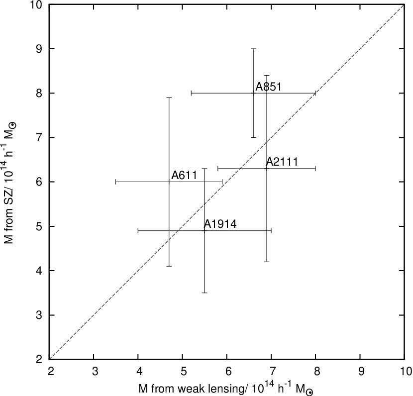
Fig. 11 shows a comparison of the different measured values of for the clusters for which we were able to perform both the SZ and lensing analyses. Measured masses for A611 and A1914 are in very good agreement. Interestingly, we find better agreement between mass measurements for A1914 than Okabe et al. (2010b), who find that including this cluster significantly distorts their otherwise well-correlated - relationship. As we use SZ measurements at rather than X-ray at , this may be indicative of SZ’s advantage in measuring the mass of merging clusters, which are likely to be more common at the higher redshifts now being probed by new galaxy cluster surveys.
We measure the mass of A851 as larger in the SZ compared to the lensing, although the difference is not a significant deviation given the errors. However it is the highest redshift cluster of the sample, it is possible that we are underestimating its mass via lensing, due to poor field galaxy selection. This may put limits on our ability to measure weak lensing at higher redshifts, at least with the two optical bands used in this analysis.
For A2111, the temperature may be somewhat higher than our - relation predicts, as this cluster is an ongoing merger and has a hot 8 keV central component; difficulties in reconciling disturbed clusters with theoretical relations have been seen in other studies (e.g. Cypriano et al. 2004). Given the small sample discussed here, it is difficult to draw general conclusions, but the technique would scale well to larger samples, from which it may be possible to correlate the state of merger with discrepancy from this - relation.
6.2 Gas distribution on large scales
The investigation of Navarro et al. (1995) into the suitability of the -model for X-ray clusters showed that the measured value of increases with increasing radius of fit. For relaxed clusters, typical values of from X-ray and high-resolution SZ, both of which resolve out large angular scales, are in the range . In the context of these core gas measurements, larger values of usually indicate merging processes.
LaRoque et al. (2006) provide the most recent combined SZ-X-ray analysis that covers the most relaxed clusters in our sample, A2111, A2259 and A611. We detect the gas masses in the similar proportions to LaRoque et al.: A611 and A2111 are of similar mass, and more massive than A2259. This is reassuring, especially given that the hot ( keV) gas in the centre of A2111 was ignored for our isothermal analysis. It is difficult to compare our values for and since we are looking at a much more extended areas of the gas and one would expect the profiles to be different for different fitting areas.
Using a -model presents a problem if extrapolated to high radii: the density does not steepen quickly enough and large, non-physical gas masses are predicted. Therefore both high- and low- angular scale measurements specify a cut-off radius at which to measure the gas mass, often , while in this analysis we use . It can be difficult to extrapolate models produced from our data to smaller radii such as , since with a high value of , our profiles may not actually reach that density before the mass goes to zero.
6.3 Gas fraction
For the most relaxed cluster in our sample, A611, we further investigated the gas fraction using a joint SZ and lensing analysis. We removed the WMAP prior on gas fraction, giving it instead a uniform prior between 0.01 and 1. The posterior plots for the model with and without the lensing data are shown in Fig. 12. Together, the datasets constrain the gas fraction, which cannot be done with either individually. It is noticeable that the SZ data has no bias in its measurement of the degeneracy; the combined data posterior lies along the posterior from the SZ data alone. This implies our parameterization is good, and that with a sensible prior on , SZ data allow us to make good estimates of cluster masses.
The combined data favour a higher value of gas fraction for this cluster than the WMAP prior normally used: compared to . However the errors are large so it is difficult to tell whether this is significant. It would be illuminating to extend this analysis to a large dataset of relaxed clusters, as general conclusions about cluster morphology cannot be made from this single result, and the other lensing-detected clusters in this paper are complex mergers.


6.4 Data issues and cluster selection
This pilot study has been helpful in identifying some areas of difficulty in joint SZ–weak-gravitational-lensing analysis. The high density of foreground optical sources in the field of A2259 made measurement of its low mass difficult via gravitational lensing, while it was well-measured via the SZ. On the other hand, the SZ analysis of A115 suffered from the effects of contaminating radio sources, and this effect is also seen in other AMI cluster observations, e.g. by AMI Consortium: Shimwell et al. (2011).
For those clusters observed outside the Galactic plane, with unresolved (easily-modelled) radio sources, the analysis showed remarkable agreement between measured regardless of dynamical state, X-ray luminosity, temperature, redshift and number of detected sub-structures. Currently the AMI Consortium has over 50 further detections of SZ clusters in similar environments covering a redshift range of and an X-ray luminosity range of W, from X-ray-selected samples. Of these, 11 have associated archival CFHT data, on which may be performed a similar analysis. Also, the clusters being discovered by Planck (Planck Collaboration, 2011a) are highly amenable to observations by AMI (AMI Consortium: Hurley-Walker et al., 2011), so there is potential to expand the sample size by another order of magnitude over coming years.
7 Conclusions
- 1.
Using AMI SZ data that measure out to , and thus probe scales comparable to those of weak-lensing observations, we have used a fast, Bayesian analysis to produce posteriors for useful parameters for six clusters, on the assumptions of an isothermal -model to SZ data and an NFW model for the lensing data;
- 2.
Of the four clusters for which we have both weak lensing and SZ data, we find that the mass estimates are in very good agreement, and that we may need to improve our field-galaxy selection for clusters at for a larger sample;
- 3.
We perform the first multiple-component weak-lensing analysis of A115 and discover significant substructure;
- 4.
We confirm the unusual separation between the gas and mass components in A1914;
- 5.
For A611, the most relaxed cluster in the sample, we have carried out a joint weak-lensing and SZ analysis with the gas fraction as a free parameter, and find that .
8 ACKNOWLEDGMENTS
We thank the staff of the Mullard Radio Astronomy Observatory for their invaluable assistance in the commissioning and operation of AMI, which is supported by Cambridge University and the STFC. Computational results were obtained using the COSMOS supercomputer (DiRAC STFC HPC Facility). This research used the facilities of the Canadian Astronomy Data Centre operated by the National Research Council of Canada with the support of the Canadian Space Agency. MLD, TMOF, CRG, MO, MPS and TWS acknowledge the support of STFC studentships.
| ID | RA | Dec | /mJy | ID | RA | Dec | /mJy | ||
|---|---|---|---|---|---|---|---|---|---|
| A | 00 56 55.18 | +26 31 24.48 | O | 00 56 01.38 | +26 28 43.78 | ||||
| B | 00 56 02.85 | +26 27 20.98 | P | 00 56 07.16 | +26 29 46.05 | ||||
| C | 00 57 21.47 | +26 17 27.90 | Q | 00 56 06.97 | +26 30 51.52 | ||||
| D | 00 55 50.46 | +26 24 39.02 | R | 00 56 00.94 | +26 25 03.79 | ||||
| E | 00 56 20.93 | +26 30 55.24 | S | 00 55 59.02 | +26 17 49.46 | ||||
| F | 00 57 06.53 | +26 25 27.03 | T | 00 56 10.64 | +26 12 03.40 | ||||
| G | 00 56 08.49 | +26 25 13.46 | U | 00 56 28.46 | +26 24 03.69 | ||||
| H | 00 56 22.47 | +26 23 03.43 | V | 00 55 58.37 | +26 25 33.95 | ||||
| I | 00 56 55.38 | +26 29 12.30 | W | 00 55 48.04 | +26 25 56.77 | ||||
| J | 00 56 18.52 | +26 05 00.41 | X | 00 56 04.35 | +26 25 00.45 | ||||
| K | 00 54 55.80 | +26 19 13.30 | Y | 00 56 05.32 | +26 23 44.74 | ||||
| L | 00 56 50.45 | +26 29 38.97 | Z | 00 56 10.69 | +26 24 15.30 | ||||
| M | 00 56 43.35 | +26 29 22.20 | AA | 00 55 49.68 | +26 22 20.83 | ||||
| N | 00 56 40.69 | +26 30 10.21 |
| ID | RA | Dec | /mJy | /mJy | ||
|---|---|---|---|---|---|---|
| A | 14 27 25.06 | +37 46 33.19 | ||||
| B | 14 25 08.41 | +37 52 42.58 | ||||
| C | 14 25 52.42 | +38 03 04.66 | ||||
| D | 14 25 40.83 | +37 45 47.93 | ||||
| E | 14 25 05.12 | +37 55 15.84 | ||||
| F | 14 27 10.92 | +37 55 13.89 | ||||
| G | 14 25 57.37 | +38 01 10.48 | ||||
| H | 14 25 47.75 | +37 47 48.32 | ||||
| I | 14 25 56.73 | +37 55 10.47 | ||||
| J | 14 25 50.36 | +37 45 07.81 | ||||
| K | 14 25 05.78 | +37 47 02.26 | – | – | ||
| L | 14 25 43.15 | +37 40 06.15 | – | – | ||
| M | 14 25 58.12 | +37 43 58.58 | – | – | ||
| N | 14 25 38.95 | +37 57 32.50 | – | – |
| ID | RA | Dec | /mJy | /mJy | ||
|---|---|---|---|---|---|---|
| A | 15 40 55.25 | +34 30 17.50 | ||||
| B | 15 38 46.64 | +34 18 58.04 | ||||
| C | 15 40 31.18 | +34 30 09.72 | ||||
| D | 15 39 11.87 | +34 29 33.07 | ||||
| E | 15 39 55.06 | +34 20 11.40 | ||||
| F | 15 40 41.89 | +34 18 35.72 | ||||
| G | 15 40 49.55 | +34 30 35.66 | ||||
| H | 15 40 31.90 | +34 28 16.52 | ||||
| I | 15 38 49.51 | +34 26 56.26 | ||||
| J | 15 39 08.11 | +34 21 09.02 | ||||
| K | 15 39 56.78 | +34 29 33.38 | ||||
| L | 15 39 30.11 | +34 29 05.46 |
| ID | RA | Dec | /mJy | /mJy | ||
|---|---|---|---|---|---|---|
| A | 17 19 13.69 | +27 44 49.47 | ||||
| B | 17 19 30.18 | +27 46 16.12 | ||||
| C | 17 20 51.25 | +27 45 08.05 | ||||
| D | 17 19 27.06 | +27 32 51.05 | ||||
| E | 17 20 20.26 | +27 28 33.96 | ||||
| F | 17 20 07.54 | +27 44 35.03 | ||||
| G | 17 19 44.57 | +27 32 37.99 | ||||
| H | 17 19 41.33 | +27 42 10.07 | ||||
| I | 17 20 16.68 | +27 37 50.27 |
| ID | RA | Dec | /mJy | /mJy | ||
|---|---|---|---|---|---|---|
| A | 08 00 07.83 | +36 04 08.56 | ||||
| B | 08 02 00.53 | +36 08 54.64 | ||||
| C | 08 00 40.55 | +36 14 23.78 | ||||
| D | 07 59 51.35 | +36 11 05.49 | ||||
| E | 08 00 43.25 | +36 14 03.44 | ||||
| F | 07 59 55.92 | +35 58 35.84 | ||||
| G | 08 02 12.27 | +36 03 48.26 | ||||
| H | 07 59 48.28 | +36 06 41.42 | ||||
| I | 08 00 03.25 | +36 00 51.74 | ||||
| J | 08 00 59.26 | +35 55 51.49 | ||||
| K | 08 01 17.11 | +36 04 31.27 | ||||
| L | 08 00 30.27 | +36 00 41.98 | ||||
| M | 08 01 24.68 | +36 05 37.48 | ||||
| N | 08 00 52.72 | +36 06 13.52 | ||||
| O | 08 00 40.14 | +35 59 51.55 | ||||
| P | 08 00 11.88 | +35 50 15.31 | — | — | ||
| Q | 08 00 54.95 | +36 17 43.76 | — | — | ||
| R | 08 00 38.30 | +36 10 56.43 | — | — |
| ID | RA | Dec | /mJy | /mJy | ||
|---|---|---|---|---|---|---|
| A | 09 44 48.36 | +47 00 02.10 | ||||
| B | 09 42 57.44 | +46 58 49.93 | ||||
| C | 09 42 34.86 | +47 18 23.55 | ||||
| D | 09 43 32.44 | +46 47 19.16 | ||||
| E | 09 43 19.30 | +46 47 32.98 | ||||
| F | 09 43 12.10 | +47 04 22.51 | ||||
| G | 09 42 24.10 | +47 02 48.19 | ||||
| H | 09 42 23.62 | +46 50 07.13 | ||||
| I | 09 42 06.14 | +46 57 05.32 | ||||
| J | 09 42 49.52 | +46 57 07.06 | ||||
| K | 09 43 00.70 | +47 01 27.71 | ||||
| L | 09 44 05.15 | +46 44 02.43 | — | — | ||
| M | 09 42 19.30 | +46 56 55.84 | — | — | ||
| N | 09 43 44.18 | +47 02 54.42 | — | — | ||
| O | 09 42 31.73 | +46 55 07.53 | — | — |
References
- Allen et al. (2003) Allen S. W., Schmidt R. W., Fabian A. C., Ebeling H., 2003, MNRAS, 342, 287
- AMI Collaboration et al. (2006) AMI Collaboration, Barker R., et al., 2006, MNRAS, 369, L1
- AMI Consortium: Davies et al. (2011) AMI Consortium: Davies M. L., et al., 2011, MNRAS, 415, 2708
- AMI Consortium: Franzen et al. (2011) AMI Consortium: Franzen T. M. O., et al., 2011, MNRAS, 415, 2699
- AMI Consortium: Hurley-Walker et al. (2011) AMI Consortium: Hurley-Walker N., et al., 2011, MNRAS, 414, L75
- AMI Consortium: Olamaie et al. (2010) AMI Consortium: Olamaie M., et al., 2010, ArXiv e-prints, 1012.4996
- AMI Consortium: Rodríguez-Gonzálvez et al. (2010) AMI Consortium: Rodríguez-Gonzálvez C., et al., 2010, ArXiv e-prints, 1011.0325
- AMI Consortium: Shimwell et al. (2010) AMI Consortium: Shimwell T. W., et al., 2010, ArXiv e-prints, 1012.4441
- AMI Consortium: Shimwell et al. (2011) —, 2011, ArXiv e-prints, 1101.5590
- AMI Consortium: Zwart et al. (2008) AMI Consortium: Zwart J. T. L., et al., 2008, MNRAS, 391, 1545
- AMI Consortium: Zwart et al. (2010) —, 2010, ArXiv e-prints, 1008.0443
- Ascaso et al. (2008) Ascaso B., Moles M., Aguerri J. A. L., Sánchez-Janssen R., Varela J., 2008, A&A, 487, 453
- Astronomical Image Processing Software (2007) Astronomical Image Processing Software, 2007, www.aips.nrao.edu
- Auld et al. (2008) Auld T., Bridges M., Hobson M. P., 2008, MNRAS, 387, 1575
- Baars et al. (1977) Baars J. W. M., Genzel R., Pauliny-Toth I. I. K., Witzel A., 1977, A&A, 61, 99
- Barrena et al. (2007) Barrena R., Boschin W., Girardi M., Spolaor M., 2007, A&A, 469, 861
- Bartelmann & Schneider (2001) Bartelmann M., Schneider P., 2001, Phys.Rep., 340, 291
- Belloni & Roeser (1996) Belloni P., Roeser H.-J., 1996, A&AS, 118, 65
- Bertin & Arnouts (1996) Bertin E., Arnouts S., 1996, A&AS, 117, 393
- Birkinshaw (1999) Birkinshaw M., 1999, Phys.Rep., 310, 97
- Bock et al. (2006) Bock D. C.-J., et al., 2006, in Society of Photo-Optical Instrumentation Engineers (SPIE) Conference Series, Vol. 6267, Society of Photo-Optical Instrumentation Engineers (SPIE) Conference Series
- Boulade et al. (2003) Boulade O., et al., 2003, in Instrument Design and Performance for Optical/Infrared Ground-based Telescopes. Edited by Iye, Masanori; Moorwood, Alan F. M. Proceedings of the SPIE, Volume 4841, pp. 72-81 (2003)., pp. 72–81
- Bridle (2001) Bridle S., 2001, in The Shapes of Galaxies and their Dark Halos, Natarajan P., ed., Proc. of the Yale Cosmology Workshop, World Scientific
- Browne et al. (1998) Browne I. W. A., Wilkinson P. N., Patnaik A. R., Wrobel J. M., 1998, MNRAS, 293, 257
- Carlstrom et al. (2002) Carlstrom J. E., Holder G. P., Reese E. D., 2002, ARA&A, 40, 643
- Cavaliere et al. (1978) Cavaliere A., Danese L., de Zotti G., 1978, in COSPAR, Plenary Meeting, Cavaliere A., Danese L., de Zotti G., eds.
- Cypriano et al. (2004) Cypriano E. S., Sodré Jr. L., Kneib J., Campusano L. E., 2004, ApJ, 613, 95
- De Filippis et al. (2003) De Filippis E., Schindler S., Castillo-Morales A., 2003, A&A, 404, 63
- Dressler et al. (1993) Dressler A., Oemler A. J., Gunn J. E., Butcher H., 1993, ApJ, 404, L45
- Dressler et al. (1999) Dressler A., Smail I., Poggianti B. M., Butcher H., Couch W. J., Ellis R. S., Oemler Jr. A., 1999, ApJS, 122, 51
- Erben et al. (2009) Erben T., et al., 2009, A&A, 493, 1197
- Feroz & Hobson (2008) Feroz F., Hobson M. P., 2008, MNRAS, 384, 449
- Feroz et al. (2009a) Feroz F., Hobson M. P., Bridges M., 2009a, MNRAS, 398, 1601
- Feroz et al. (2009b) Feroz F., Hobson M. P., Zwart J. T. L., Saunders R. D. E., Grainge K. J. B., 2009b, MNRAS, 398, 2049
- Giovannini et al. (1987) Giovannini G., Feretti L., Gregorini L., 1987, A&AS, 69, 171
- Govoni et al. (2001) Govoni F., Feretti L., Giovannini G., Böhringer H., Reiprich T. H., Murgia M., 2001, A&A, 376, 803
- Govoni et al. (2004) Govoni F., Markevitch M., Vikhlinin A., VanSpeybroeck L., Feretti L., Giovannini G., 2004, ApJ, 605, 695
- Gutierrez & Krawczynski (2005) Gutierrez K., Krawczynski H., 2005, ApJ, 619, 161
- Hoekstra et al. (2000) Hoekstra H., Franx M., Kuijken K., 2000, ApJ, 532, 88
- Hoekstra & Jain (2008) Hoekstra H., Jain B., 2008, Annual Review of Nuclear and Particle Science, 58, 99
- Iye et al. (2000) Iye M., et al., 2000, PASJ, 52, 9
- Komatsu et al. (2011) Komatsu E., et al., 2011, ApJS, 192, 18
- LaRoque et al. (2006) LaRoque S. J., Bonamente M., Carlstrom J. E., Joy M. K., Nagai D., Reese E. D., Dawson K. S., 2006, ApJ, 652, 917
- Marshall et al. (2002) Marshall P. J., Hobson M. P., Gull S. F., Bridle S. L., 2002, MNRAS, 335, 1037
- Marshall et al. (2003) Marshall P. J., Hobson M. P., Slosar A., 2003, MNRAS, 346, 489
- Meneghetti et al. (2003) Meneghetti M., Bartelmann M., Moscardini L., 2003, MNRAS, 340, 105
- Miller et al. (2006) Miller N. A., Oegerle W. R., Hill J. M., 2006, AJ, 131, 2426
- Navarro et al. (1995) Navarro J. F., Frenk C. S., White S. D. M., 1995, MNRAS, 275, 720
- Okabe et al. (2010a) Okabe N., Takada M., Umetsu K., Futamase T., Smith G. P., 2010a, PASJ, 62, 811
- Okabe & Umetsu (2008) Okabe N., Umetsu K., 2008, PASJ, 60, 345
- Okabe et al. (2010b) Okabe N., Zhang Y., Finoguenov A., Takada M., Smith G. P., Umetsu K., Futamase T., 2010b, ApJ, 721, 875
- Patnaik et al. (1992) Patnaik A. R., Browne I. W. A., Wilkinson P. N., Wrobel J. M., 1992, MNRAS, 254, 655
- Planck Collaboration (2011a) Planck Collaboration, 2011a, ArXiv e-prints, 1101.2024
- Planck Collaboration (2011b) —, 2011b, ArXiv e-prints, 1101.2022
- Romano et al. (2010) Romano A., et al., 2010, A&A, 514, A88+
- Schneider et al. (2006) Schneider P., Kochanek C. S., Wambsganss J., 2006, Gravitational lensing: strong, weak and micro. Springer
- Seitz et al. (1996) Seitz C., Kneib J.-P., Schneider P., Seitz S., 1996, A&A, 314, 707
- Skilling (2004) Skilling J., 2004, in American Institute of Physics Conference Series, Fischer R., Preuss R., Toussaint U. V., eds., Vol. 735
- Stott et al. (2008) Stott J. P., Edge A. C., Smith G. P., Swinbank A. M., Ebeling H., 2008, MNRAS, 384, 1502
- Sweeney (2006) Sweeney D. W., 2006, in Society of Photo-Optical Instrumentation Engineers (SPIE) Conference Series, Vol. 6267, Society of Photo-Optical Instrumentation Engineers (SPIE) Conference Series, pp. 6–8
- Swetz et al. (2011) Swetz D. S., et al., 2011, ApJS, 194, 41
- The Dark Energy Survey Collaboration (2005) The Dark Energy Survey Collaboration, 2005, ArXiv e-prints, 0510346
- Vanderlinde et al. (2010) Vanderlinde K., et al., 2010, ApJ, 722, 1180
- Waldram et al. (2003) Waldram E. M., Pooley G. G., Grainge K. J. B., Jones M. E., Saunders R. D. E., Scott P. F., Taylor A. C., 2003, MNRAS, 342, 915
- Wang et al. (1997) Wang Q. D., Ulmer M. P., Lavery R. J., 1997, MNRAS, 288, 702
- Wilkinson et al. (1998) Wilkinson P. N., Browne I. W. A., Patnaik A. R., Wrobel J. M., Sorathia B., 1998, MNRAS, 300, 790