Transport properties of 3D extended -wave states in Fe-based superconductors
Abstract
The Fermi surfaces of Fe-pnictide superconductors are fairly two-dimensional (2D), and it has thus come as a surprise that recent penetration depth and thermal conductivity measurements on systems of the 122 type have reported -axis transport coefficients at low temperatures in the superconducting state comparable to or even larger than that in the -plane. These results should provide important information on both the Fermi surface and the superconducting state. Here we consider the theory of the superfluid density and thermal conductivity in models of extended- wave superconducting states expected to be appropriate for Fe-pnictide systems. We include intraband disorder and consider a range of different Fermi surfaces where gap nodes might exist. We show that recent experiments on Ba(Fe1-xCox)2As2 can be semiquantitatively understood by such an approach, and discuss their implications.
I Introduction
The new Fe-based superconductors have captured the imagination of the theoretical and experimental superconductivity community, in part because the critical temperature is high in certain materials, but also because the phenomenology of the superconducting state appears to be quite different from any class of novel superconductors heretofore discovered [1, 2]. Since calculations of the coupling strength due to the electron-phonon interaction show it to be small [3, 4, 5], it is believed that electronic pairing is predominant; thus attention has focussed on sign-changing states with symmetry predicted by spin fluctuation theory [6, 7, 8, 9, 10, 11, 12]. Depending on the details of the microscopic pair interaction[9, 13, 14] such states may display “accidental” nodal structures, nodes not dictated by symmetry considerations. It is important to understand such structures, as they provide clues to the origin of pairing.
In the LaFePO, KFe2As2, and BaFe2(As1-xPx)2 systems there is considerable evidence for low-energy excitations which could be produced by order parameters with nodes, but the structure of the nodal manifold is still controversial. In the heavily-studied Ba(Fe1-xCox)2As2, Ba(Fe1-xNix)2As2 and BaFe2(As1-xKx)2 systems, which we will refer to collectively as Ba-122, measurements have been interpreted variously in terms of fully gapped behavior, deep minima in the superconducting gap, or gap nodes, and there is some evidence that these conclusions may be quite doping-dependent. The experimental probe which has thus far provided the lowest temperature information on the bulk order parameter is thermal conductivity. In the 122 systems, the -plane thermal conductivity data exhibited zero or extremely small linear- term in zero magnetic field, reflecting the apparent absence of any nodes in the superconducting gap. The field dependence, however, was significantly stronger than that expected for a large-gap superconductor[15, 16, 17]. This was analyzed by Mishra et al.[18] in terms of a gap with A1g symmetry with no nodes but deep minima on the electron sheets. Bang proposed that this effect could also be explained phenomenologically by an isotropic state with very small gap on one Fermi surface sheet[19].
Recently, Martin et al.[20] reported a strong linear- behavior of the magnetic penetration depth for currents along the -axis in overdoped Ba(Fe1-xNix)2As2crystals, compared to a predominantly behavior in the -plane, with possible much smaller linear- contributions for some dopings. These authors pointed to a need for theoretical analysis of superconductivity in these materials beyond 2D models. Subsequently Reid et al.[21] measured a significant linear- term in the low- -axis thermal conductivity of Ba(Fe1-xCox)2As2crystals, compared to a smaller or zero linear term in the -plane. In addition, the anisotropy ratio of the electronic thermal conductivities normalized to their values at determined via resistivity measurements and the Wiedemann-Franz law, was found to increase rapidly as the crystal was doped away from optimal . These authors argued that such an anisotropy ratio could arise only from gap nodes located precisely at flared regions of the quasi-cylindrical Fermi surfaces where , such that the corresponding arising at low from the nodal structures would be negligible.
For some samples, Reid et al. reported a nonzero limiting value of of order 1 W/K2cm. It is important to note that these values are much smaller than the value predicted in the simple BCS theory of quasiparticle transport in a nodal superconductor, of order , where is the Fermi level density of states, is the Fermi velocity and is the gap velocity . This value is also much smaller than that observed in the cuprate case[22]. The low- linear term in the thermal conductivity is expected to be universal (disorder-independent for weak disorder) in the -wave or -wave case[23, 24]. Mishra et al.[18] showed recently that this expression continues to hold in the extended- type states thought to be characteristic of Fe-pnictide systems, but that universality breaks down effectively due to the strong dependence of on disorder.
Theory has also made some recent progress in dealing with deviations from pure 2D behavior. Early spin fluctuation calculations for the pairing state of the Fe-pnictide materials [6, 7, 10, 25] found that, depending on details of electronic structure and interaction parameters, nodes could occur on the electron sheets, but the gap on the hole sheets was always fairly large and isotropic. On the other hand, Graser et al.[26] recently presented a calculation of spin-fluctuation pairing in the 122 systems based on an RPA treatment of a 5-orbital model derived from density functional theory (DFT) electronic structure. In some cases, particularly for substantial hole doping, the ground state was found to be of symmetry, as in the 2D case, but while the electron sheet gap was found to be highly anisotropic but nodeless, the hole sheet was found to have nodes near the top of the Brillouin zone near the point where the Fermi surface sheets experience some outward flaring. Similar results were subsequently obtained by Kuroki et al. for BaFe2(As1-xPx)2[27].
In this work, we consider various possible Fermi surface geometries and gap structures which may give rise to the unusual low transport anisotropy seen in Refs. 28, 21, bearing in mind that any phenomenology which purports to explain the results of these works must also be consistent with the earlier thermal conductivity results of Refs. 15, 16, 17. Although we consider 3D order parameter structures of the type found in Graser et al.[26], we do not attempt to tie our calculations or parameters to any particular microscopic calculation of either the Fermi surface or gap function, but rather to place restrictions on what types of structures are possible on the basis of these measurements. We argue that gap structures with small nodal segments near the sections of flared Fermi surfaces are the most likely way to explain the unusual anisotropy in , the small size of these linear terms, and the magnetic field dependence observed. To some extent our calculations also depend on the role of disorder in these materials, which is not completely understood. In Section II, we present the model we study, in Section III give our results, in Section IV discuss them in comparison with experiment, and in Section V, conclude and critically consider the limitations of our approach.
II Model
II.1 Fermi surfaces and gap structures
The purpose of this study is to examine transport in the superconducting state at very low energies; to this end, only the structure of the Bogliubov quasiparticle spectrum near gap nodes or deep minima is relevant. In theoretical studies of these systems performed thus far, nodal structures in states have been obtained on either electron or hole pockets, but not both. We therefore consider two Fermi surface sheets, one of which () possesses gap nodes. The second () will be assumed to have deep gap minima, or to be irrelevant altogether for extremely low-energy transport. Results are symmetrized to ensure invariance under point group rotations. For the 122 systems, we will have in mind primarily that sheet is one of the hole sheets[26] and that is the (properly symmetrized) electron sheet. The reason is that, to the extent that nodes are occasionally found in spin fluctuation calculations on the electron sheets, they tend to run vertically from bottom to top of the Brillouin zone, and would therefore lead to an extremely large thermal conductivity anisotropy , in apparent contradiction to experiment. However, none of the results actually depend on the assignment of and .
Fig. 1 shows various different kinds of Fermi surfaces and nodal structures which we consider in this work. Among the figures labeled “”, example 1 is a Fermi surface fit to the hole-doped sheet of Ref. 26, calculated using a 5-orbital fit to a first principles calculation for BaFe2As2 using the Quantum ESPRESSO package, assuming fixed experimentally determined atomic positions in the unit cell. The nodal line structures considered here are typical of the 3D ground states found on the and sheets in that work. Example 2 is the same Fermi surface with horizontal nodes found in the same case in Ref. 26 on the sheet. Example 3 is a model Fermi surface with identical topology but increased flaring near the top and bottom zone faces, with assumed V-shaped nodes near the flared portion. This Fermi surface is obtained within the same calculational scheme[26] for the Fermi surface, but using a structural optimization of the internal coordinate of the As position. In both calculations we have used Å and Å. Similar results are found elsewhere[29, 30, 31]. ARPES has provided some evidence for flaring of hole Fermi surfaces with large near the zone top [32, 33, 34, 35], increasing with Co concentration, but at this writing there is no complete consensus on the 3D Fermi surface of the doped materials. Example 4 is the same Fermi surface but with horizontal nodes close to the value where takes on a maximum. Example 5 is a model surface similar to that found in density functional theory calculations upon electron doping of the sheet together with a model gap structure giving nodes on the top surface. Finally, the last panel in Fig. 1 shows the second sheet , fit to the Quantum ESPRESSO calculation for the electron sheets of BaFe2As2 for unrelaxed As coordinate, which is assumed to exist together with each of the cases 1-5 for . We emphasize that our point of view here is that of phenomenologists; we allow ourselves to ask what would be the consequences if the Fermi surfaces actually took the forms shown for any of the doped materials.
A crucial ingredient in the calculations presented below are the Fermi velocities near the nodal surfaces. In Table 1, we list some values of Fermi velocity components and certain averages which will be important in the discussion below for the various cases for sheet and our fixed choice of . The dependence of the Fermi velocity components is exhibited in Figure 1.
| 1.977 | 1.977 | 1.826 | 1.826 | 1.74 | 3.021 | |
| 0.293 | 0.293 | 1.277 | 1.277 | 0.683 | 0.562 | |
| 2.074 | 2.037 | 2.076 | 1.546 | 1.067 | ||
| 0.473 | 0.433 | 1.197 | 2.591 | 0.792 | ||
| 0.9 | -1.4 | 0.9 | 1.2 | 1.1 | 0.9 | |
| -8.6 | 9.1 | -8.6 | -9.4 | -8.4 | 1.5 |


In calculations of observables presented below, we have reduced all Fermi velocities shown in Table 1 by a factor of 4 to account for the effective renormalization of the bands with respect to DFT seen in ARPES which appears to be between 1.5 and 6 for all Fe-based superconducting materials[33, 36]. There may be an additional low-energy renormalization at the meV scale, as discussed by Benfatto et al.[37]. All of these many body effects are lumped into a single doping– and momentum–independent renormalization of the Fermi velocity here, to get the crudest description of the anisotropy of transport properties driven by the underlying anisotropy of the DFT Fermi surface.
The model we adopt for the order parameter is a 3D extension of the phenomenological form treated, e.g. in Ref. 18. To obtain strictly horizontal nodes (cases 2,4,5), we consider gaps of the form
| (1) |
whereas V-shaped nodal structures (cases 1,3) similar to that found in Ref. 26 (see Fig. 1) are produced by
| (2) |
with for the first kind of order parameter and for the second kind of order parameter. In Fig. 1 for simplicity we have shown only the nodal surfaces of the order parameters chosen on the various Fermi surfaces, together with the variation of the Fermi velocity on those surfaces as a function of .
II.2 Disorder in 2-sheet pairing model
For disorder, we will assume an orbital-independent matrix element which scatters quasiparticles either within a given band with amplitude , , or between bands with amplitude . We sum all single-site scattering processes of arbitrary strength to obtain a disorder-averaged Nambu self energy , where is the concentration of impurities, and is the impurity -matrix as parameterized e.g. in Ref. 18. For simplicity, we assume , with equal densities of states throughout the paper. In our preliminary considerations we restrict ourselves to purely intraband scattering, . The disorder is characterized by two intraband scattering parameters on each sheet: and ; For our simple initial case with 2 symmetric bands we set and , . We only consider intraband scattering in the unitary limit [38], and further note that nonzero interband scattering does not affect the physics qualitatively, unless the interband scattering is as strong as the intraband scattering[39]. In presence of such strong isotropic scattering, one would expect a large suppression of which is not observed in experiments.
The disorder-averaged matrix Green’s function in the presence of scattering in the superconducting state is given by a diagonal matrix in band space,
| (3) |
where is restricted to Fermi surface sheet with , and the renormalized quantities , , also depend on the band indices through . The are the components of the self-energy proportional to the Pauli matrices in particle-hole (Nambu) space.
III Results
III.1 DOS
Below we focus on several bulk observables. It is useful to start with the analysis of the total density of quasiparticle states (DOS)
| (4) |
where the momentum summation indicates the explicit integration over distinct Fermi surface sheets with momenta . The total residual density of states (DOS) at the Fermi level contains vital information about the low lying quasiparticle excitations and will determine all leading low temperature power laws. This quantity is sensitive to disorder or magnetic field. To give the reader a sense of the average density of quasiparticle excitations without reference to Fermi surface anisotropy, we calculate the residual DOS as a function of normal state scattering rate due to intraband disorder. Figure 2 shows for the five different cases in consideration; generally it first increases with disorder, attains a maximum value and rapidly drops to zero again. This “re-entrant” gapped behavior is a consequence of the node lifting phenomena characteristic of accidental nodes in an order parameter with A1g symmetry[40, 18]. Considering the evidence provided by Refs. 20, 21 for low-energy excitations, we assume in our discussion below that we are in the regime with nodes and no true gap in the system. The values of the scattering rate for “dirty” systems presented here are chosen in each case to correspond to the maximum residual DOS induced by disorder as shown in Fig. 2. In all cases we have verified that the corresponding suppression relative to the pure system is (1%) or less for all cases.
We note that for the various cases considered, the node-lifting process can take place at quite different rates. In particular, the nodes on the top of the closed Fermi sheet in case 5 are quite sensitive to a very small amount of disorder. The sensitivity of this case to disorder is the strongest argument against an explanation of the Reid et al. data based on a Fermi surface and state of type 5.


III.2 Penetration depth
The London penetration depth for currents flowing in the th direction is a fundamental measure of the superconductivity and is related to the superfluid density by . The superfluid density tensor is related to the total electromagnetic response of the system to an external field in the limit. For a general multiband dispersion and in presence of the impurities, one finds that the penetration depth is given by the expression
| (5) | |||||
where is the distance between planes, the index denotes the band and stands for the current direction or and is an average over the Fermi surface. In the absence of disorder, this expression reduces to the result for the superfluid density of a clean system with general band found, e.g. in Ref. 41. The second term in Eq. (5) contains the nodal gap slope , which is extremely small compared to the Fermi velocity, and will be neglected in our calculations. Most experiments measure the change in the penetration depth from some minimum temperature , and are not sensitive to the absolute value of the penetration depth.
| Case | (nm) | (nm) |
|---|---|---|
| 1,2 | 87 | 334 |
| 3,4 | 87 | 287 |
| 5 | 87 | 329 |
Note that since we begin from a realistic Fermi surface and assume a as appropriate for the Co-doped 122 systems, the reader might assume that we are in a position to calculate on an absolute length scale the zero temperature penetration depth . Indeed the expression (5) reduces at to
| (6) |
which gives the correct result in the limit of a single parabolic band. However a closer examination of Eq. (5) reveals that the integrand determining extends over all occupied bands, i.e. it involves the full electronic structure and not just the Fermi velocities, whereas in Eq. (5) we have linearized the band structure near the Fermi level for simplicity. Thus we are not able to use Eq. (5) to obtain accurate estimates of even if the input band structure was perfectly correct. By contrast, the integrand determining
| (7) |
is sharply peaked at the Fermi level, and so may be calculated accurately. Even in this case, however, the overall scale is set by . The usual procedure would be to take from optical experiments. Indeed, in these systems the -plane penetration depth is of order 200-450 nm [42, 43, 44, 45, 46, 47], but there are no reported measurements of of which we are aware. For purposes of this work we use ’s determined from Eq. (6) (given for completeness in table 2) to fix the scale of . The overall length scale of field penetration may therefore be incorrect by up to a factor of two, but the -dependence should be calculated accurately.
The temperature correction is often used as a probe of the nodal structure of gaps in unconventional superconductors[48]. In general, the asymptotic power laws for systems with line nodes are for a clean and for a dirty system [49], but the range of validity of these results may be experimentally unobservable depending on the form of the impurity scattering and the detailed momentum dependence of the superconducting gap. In our current calculations with intraband impurity scattering only, the concentrations have been chosen in order to minimize suppression; the corresponding density of states and size of the asymptotic terms are therefore quite small, and the latter is not clearly visible in Fig. 3. On the scale of the Figure shown, these asymptotic power laws are modified by low energy scales associated with both sheets and , as well as the significant energy dependence of the impurity self-energy. Over an experimentally relevant range, a wide range of “best fit” power laws are therefore a priori possible.
In Fig. 3, we show as a function of temperature for the various cases we consider here. The size of the observable quantity is seen to be in reasonable agreement with the measured penetration depth changes in recent measurements in optimal to overdoped Ba-122[28]. The scale of is significantly larger than , due to the much larger .
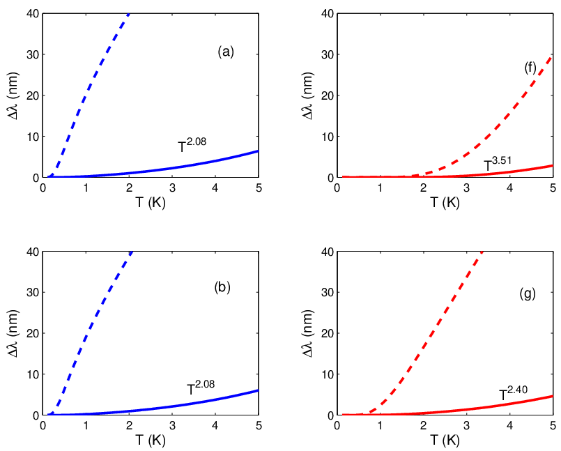
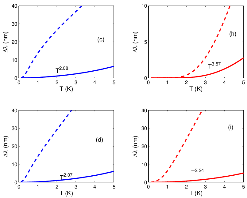
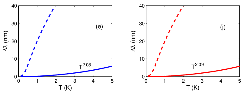
In addition, Figure 3 shows qualitatively different behavior for -plane and -axis penetration depths. These results, particularly those for cases 3 and 4, are in qualitative agreement with experimental measurements on Ni doped 122 compounds, where linear behavior along the -axis and power law behavior for -plane with exponent for concentrations =0.03 to 0.07 (only those above are outside the spin density wave (SDW) state)[20] were reported. For Co doped 122 systems, we are not aware of any -axis penetration depth measurements.
The -plane penetration depth data in 122 systems has been reported for some time now to be close to a power law with an exponent of about 2. It has usually been assumed that this result is obtained due to impurity scattering, either in a nodal system[18] or in a fully gapped state with interband scattering such that midgap bound states are formed[50]. These effects may indeed be present in very dirty samples. However, the existence of a linear- term for the -axis penetration depth suggests that this simple argument cannot be the complete explanation for the approximate behavior in the better samples; were the system sufficiently dirty to show behavior in the -plane, it would perforce manifest the same behavior for currents in the -axis direction (we ignore for the moment the possibility that impurity scattering is itself highly anisotropic with respect to the directions.). The difference in power laws in the two directions must therefore be ascribed to some other effect or combination of effects. In our proposal, there is no true behavior except perhaps at the very lowest temperatures; the upward curvature observed over a range of several Kelvin is due in part to the “activation” of a new source of quasiparticle excitations as the temperature is increased. At low temperature all quasiparticles come from sheet , since we have assumed that this is the only sheet where true nodal excitations exist. On the other hand the order parameter on the sheet is assumed to have deep minima . When exceeds this scale, quasiparticles from this sheet may be excited and a new contribution (upward curvature) to appears. Since is assumed to have smaller , it does not contribute significantly to , however. The second cause of “power law” behavior is indeed the disorder, but it is impossible to make universal statements about the large ranges over which experiments are typically fit. To give a more useful measure of the form of these results in Fig. 3, we have performed best fits of the dependence to over the finite range of temperatures shown.
The penetration depth anisotropy
| (8) |
has been claimed in Refs. 51, 52 to be of order 3-6 at low temperature, and to decrease weakly with increasing temperature, but cannot yet be measured directly. Experimentally, is measured, and must be combined with measurements of , with to determine the anisotropy ratio. Reliable measurements of from, e.g. optics experiments, are not yet available for the 122 materials to our knowledge. However, within our theoretical framework can be determined, with the caveats described above, and Fig. 4 shows for the different cases. We therefore regard this as a prediction of weakly increasing with temperature which may be verified at the point that reliable values of are obtained from optics or elsewhere.
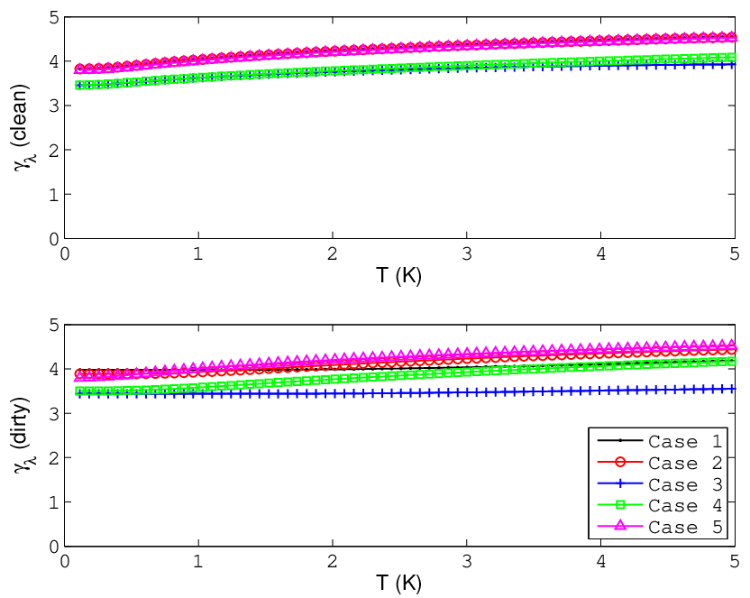
Our results are in the range of anisotropy ratios deduced from experiment[51], but increase weakly rather than decrease weakly with temperature at low temperatures. A glance at the approximate inequality in Eq. (8) shows that a somewhat smaller value of than effectively assumed in Refs. 51, 52 would bring the measured ’s and therefore the -dependence of in agreement with our results.
We can now ask which type of Fermi surface/order parameter combination represents the experimental penetration depth data best. For cases 1 and 2, the -axis Fermi velocity is small, which means not only that is smaller at low , where it derives entirely from the nodes, but also that the contribution from the deep minima is correspondingly more important; as seen in Fig. 3, for these cases the -axis penetration depth as a function of has substantial upward curvature, which is never observed in experiment. Power law fits to the -plane results give exponents which tend to be too close to 1. On the other hand for cases 3 and 4, has no upward curvature above a scale corresponding to approximately and is quasilinear over a significant range, while displays power law behavior with approaching 2 in the dirty cases shown over a finite range, as observed in experiment. Case 5 displays a large penetration depth anisotropy, but an anomalous dependence which is due to the extremely small for this case which must be chosen to place the nodes in a position with high . Therefore from the point of view of the penetration depth temperature dependence and crude anisotropy, only cases 3 and 4 appear compatible with experiment. We emphasize again that the power laws stated in Fig. 3 are phenomenological fits and are not exact in any asymptotic limit. Exponents may be expected to change as the low energy gap scales are changed, and in particular to increase somewhat as interband scattering is added.
Before closing this section, we note that nonlocal electrodynamics are unlikely to play a significant role in these measurements. This is because the typical energy scale which cuts off singularities in nodal superconductors is . For both directions in the 122 samples, this scale is of order a few tenths of Kelvin or less. The crossover in clean samples from linear to from nonlocal effects will therefore only complicate interpretations at unobservably low temperatures, where disorder will probably dominate in any case.
III.3 Thermal conductivity in zero magnetic field
The electronic thermal conductivity is calculated here using a straightforward extension of the standard approach[53, 54, 55] to multiband superconductors[18]. In the presence of disorder, we evaluate the expression arising from the electronic heat current bubble,
| (9) | |||||
where
| (10) |
and , is the band mass, is the Fermi velocity on the th band, and . Terms involving the gap slope at the nodes are numerically negligible since and are omitted in our evaluations. Here, is an average over each Fermi surface sheet, denotes the sum over the bands, is the Fermi velocity on sheet , and is the number of FeAs planes per unit cell.
We focus first on the linear term in in the limit, the only experimentally unambiguous signature of purely electronic heat transport by nodal excitations. In the limit , Eq. (9) reduces to
| (11) |
where is a dimensionless constant, is the number of distinct nodal surfaces, assumed equivalent, and is the effective mass for motion of quasiparticles in the -plane. The result obtains exactly only if and are constant over the entire nodal surface, which is unrealistic except, crudely speaking, in a 2D situation, but if the velocities are replaced by the average expression of Eq. (11) will give a reasonable result. The constant reduces to in the well-known case of a 2D -wave order parameter, and will be of the same order of magnitude for a clean nodal state if the nodes are vertical and run the length of the Fermi cylinder. In any situations where the nodal lines do not span the dimensions of the Fermi sheet, i.e. consist of small circles or segments, as in all the cases for considered in Fig. 1, the factor contains the relative nodal phase space and will therefore be . Note that in the -wave and certain -wave cases, the result of Eq. (11) is also universal, in the sense that the nodal velocities are unrenormalized by disorder [23, 24], but in the generalized case this universality breaks down [18].
It is instructive to compare crude estimates of what one might expect for with actual theoretical results and the experimentally measured values. In Table 3 we first show progressively more accurate estimates of this quantity. First, we remark that a small linear- term in must be present if nodes are present and if has any nonzero component in the -plane. To be consistent with earlier data and with the recent work of Reid et al.[21] in the Co-doped Ba-122 system, this term must be quite small, consistent with zero within the resolution of the experiment, at least near optimal doping. It is clear from the table that a 2D -wave state or, equivalently, an anisotropic nodal -wave state with line nodes running the length of the Fermi cylinder (“method T1”) would dramatically overestimate the experimental results for in the ab plane. The best estimate based on Eq. (11) (“method T2”), accounting for realistic values of nodal velocities , still gives a value significantly larger than experiment near optimal doping in the Ba(Fe1-xCox)2As2 system studied by Reid et al. as shown in Table 3. This is at least in part because method T2 also does not account for the small nodal phase space. The T3 column of Table 3 shows the clean limit of the exact numerical evaluation of Eq. (9) for the 5 cases. These results are now of order the scatter in the data (consistent with zero) of the -plane linear- terms in identified in samples near optimal doping by Reid et al., which we take to be the resolution of the experiment, about W/K2cm.
| Theory | Ba(Fe1-xCox)2As2 | LFPO | P-122 | ||||||
|---|---|---|---|---|---|---|---|---|---|
| Case | T1 | T2 | T3 | 0.074 | 0.108 | 0.114 | 0.127 | ||
| 1 | 118 | 31 | 1.8 | ||||||
| 2 | 118 | 71 | 3.1 | ||||||
| 3 | 102 | 31 | 2.5 | 0 | 0 | 0 | 17 | 3000 | 250 |
| 4 | 102 | 59 | 6.3 | (-1,3) | (-1) | (-9,-13) | |||
| 5 | 94 | 47 | 3.1 | ||||||


Depending on the Fermi surface, the corresponding -axis transport can be smaller or larger than the -plane results discussed. To illustrate the qualitative anisotropy found here, we plot in Fig. 5 the -plane and -axis thermal conductivities for increasing intraband impurity scattering. There are several interesting points in this Figure. First, we note that for cases 1 and 2, where the Fermi surfaces are nearly cylindrical, the -plane conductivity is much larger than the -axis conductivity. Clearly again these cases are inconsistent with experiment. For the more flared Fermi surface, cases 3 and 4, it is possible to have and comparable, or even have . Note this is more likely for the horizontal line nodes of case 4, which have been chosen to lie at the maximum value of for this Fermi surface, whereas the V-shaped nodes of case 3 sample the high values less often. A large anisotropy is also observed in case 5 for reasons similar to those of case 4.
As intraband scattering is increased, a constant term is added to the off-diagonal self-energy in Nambu space[18] which eventually lifts the nodes, as seen in the DOS (Fig. 2). As this occurs, two effects happen in parallel: a) decreases; and b) the nodal surfaces (which are shown in Fig. 1 for the clean system only) move towards the top and bottom of the Brillouin zone, respectively. The latter effect can increase or decrease the thermal conductivity depending on whether or not the node-lifting process moves the nodes towards regions of higher or lower . Thus, depending on details, the / anisotropy can be enhanced or suppressed by disorder.
In Ref. 21, the authors specifically discuss the normalized measure of thermal conductivity anisotropy , and demonstrate that this ratio has a minimum at optimal doping. This result should be treated with caution, however, both because a) the linear term in is consistent with zero for much of the doping range; and b) the normal state ’s are determined by measurement of the resistivity extrapolated to and use of the Wiedemann-Franz law. However, if the elastic transport scattering rate is reasonably isotropic, as seems likely, will be determined simply by the ratio
| (12) |
where is the average of the Fermi velocity components over the nodal manifold. Here we calculate within a simple model where normal state heat conduction is controlled by (isotropic) intraband impurity scattering only. In Fig. 6, we show that only for cases 3-5 it is possible to achieve values of substantially greater than 1. For case 5, the node lifting scattering rate is minuscule in absolute units, such that we rule out this case as well, provided our assumption that intraband scattering dominates is correct.
An alternate possibility to create a small residual would be the creation of an impurity band in a gapped state due to interband scattering[18], but in this case there is no natural reason to have a transport anisotropy other than that given by , which for all cases discussed here would give a very strong dominance by the -plane thermal currents on an absolute scale, and would lead to in all samples, in contrast to experiment.
III.4 Magnetic field dependence of


The final notable feature seen in experiment[17, 21] is an unexpectedly large enhancement of the in-plane residual term in the presence of a magnetic field along the -axis. With moderate magnetic field of a few Tesla, the residual in-plane term becomes comparable to the -axis term , and both exhibit a field dependence with downward curvature reminiscent of the presence of field-induced residual quasiparticle excitations contributing to the thermal current[58]. This effect was discussed already for the -plane thermal conductivity in Ref. 18, where it was concluded that the most likely origin of the strong field dependence in apparently fully gapped samples was contributions from deep minima in the gap on the electron sheets, as found in early multiorbital spin fluctuation theories[12, 13, 7, 59, 10]. Note that in the 3D spin fluctuation analysis of Graser et al.[26], these deep minima on the electron sheets continue to exist, and run the entire length of the Fermi cylinders, thus providing much more phase space than at zero field, as soon as the magnetic field energy spans the very small minimum gap . Thus the thermal conductivity, negligible in zero field, can jump fairly rapidly[39].
To include the presence of magnetic field explicitly, in this work we use the standard semiclassical (Doppler shift) method[60, 58, 61, 62], where the quasiparticle energy is modified by its Doppler shift in the local superfluid flow field. While this approach is never exact[63], it provides a good qualitative description of the magnetic field dependence of the quasiparticle properties of nodal superconductors over a wide field range[64]. The local Doppler shift of a quasiparticle with momentum (band indices are suppressed) is
| (13) |
where is the local supercurrent momentum, approximated for a single vortex as
| (14) |
Here is the distance from the vortex core and is the vortex winding angle. In the presence of the magnetic field, we replace by in Eq. (9). In this approach, any physical quantity is calculated in the usual way with Doppler shifted energy, and the averaging is performed over a unit cell of the vortex lattice, approximated as circular, as
| (15) |
where is the local (Doppler shifted) result from Eq. (9), is the magnetic length scale, with the superconducting flux quantum. For lower fields , this is a qualitatively good approximation. Somewhat more sophisticated approximations can be obtained within the semiclassical framework[62], but the above will suffice for our qualitative purposes. Here is the upper critical field and is the coherence length.
Using this method, we now calculate the low- residual thermal conductivity in both directions as a function of the magnetic field. Fig. 7 shows the field dependence of the residual linear term, which is similar to a superconductor with nodes, for both directions of the heat current, with the magnetic field taken always to point along the -axis as in experiment. Note that in principle the situations with heat current parallel and perpendicular to the field are physically different regardless of the orientation of the crystal axes: in one case the heat current flows down the axis of a vortex and may be assumed to sample a single , while in the other case it samples a modulated across the vortex lattice. This averaging problem for the perpendicular heat flow has never been addressed in a completely convincing fashion. We therefore present two extremes of the possible field dependence for currents in the the -plane: first, a “parallel average” over the vortex flow field , where represents a direct average over the vortex unit cell as in Eq. (15); second, a “series average”, , as discussed in Ref. 58. We note that the results for the Brandt-Pesch-Tewordt average Green’s function theory[39] appear to lie closer to the parallel average.
Fig. 7 shows several interesting effects. First of all, while the Fermi surfaces with less flaring (cases 1 and 2) displayed much larger values of the absolute -plane thermal conductivity in zero field (Fig. 5, panels (a) and (b)) than the more flared cases 3 and 4 (Fig. 5, panels (c) and (d)), the -plane field dependence at any reasonable field is seen to dominate the absolute -axis response for all cases 1-4 (Fig. 7, panels (a-d)). This is because we have assumed, as in Ref. 39, that the sheet has a deep gap minimum, spanned by the Doppler field energy at a field of only 1.2 T. Note this is an average scale over the entire sheet; the dispersion of the Fermi velocity with leads to a smearing of any feature associated with this scale. It is these long deep gap minima on (putative electron sheets) which dominate the field response in this case, with subdominant contributions from the (putative hole sheets) above this field range. Because , it is still possible to have a normalized thermal conductivity larger in the -axis direction (Fig. 7, panels (f) and (g)).

The Reid et al. experiment Ref. 21 shows a pronounced tendency for the normalized anisotropy ratio to fall rapidly from large values as a function of magnetic field, and then to saturate at values of order 1 when fields of a few Tesla are reached. Within our calculational scheme, such a conclusion is quite natural since the zero-field anisotropy (Fig. 6) is dominated by the weak nodes on the sheet(s), which can give large ’s, particularly in cases 3 and 4, as discussed above. On the other hand, as the field is switched on, the contributions of the deep gap minima on the sheets come into play, and indeed dominate for sufficiently large fields because of the much larger phase space of the gap minima on compared to the phase space taken by the gap nodes on . If a single 2D sheet dominates the field dependence, the normalized anisotropy ratio will reduce to approximately 1 since the Fermi velocity anisotropy has been removed by the normalization, provided the averaging over the vortex lattice is performed identically for in-plane and -axis currents. This behavior is seen in Figure 8, where the inverse of the anisotropy ratio, is plotted to facilitate comparison with experiment. If series-type averaging is more appropriate in the -plane, the high-field can be considerably larger, as also seen in Figure 8.
III.5 Doping dependence
Within our current crude approach, doping is accomplished by rigidly shifting the chemical potential relative to the parent compound. However, the dependence of the Fermi surface thus obtained is consistent neither with that observed in ARPES experiments on 122 compounds nor with virtual crystal approximation within DFT calculations. In particular, the flaring of the hole () Fermi surface upon electron doping does not increase rapidly with electron doping, as seen in ARPES and DFT calculations[33, 36]. In this section we therefore investigate, independently of any microscopic model of the band structure, the effect on superconducting state transport of the flaring of the Fermi surface. To this end, we simply interpolate the Fermi surfaces between cases (1,2) and (3,4), and calculate the thermal conductivity as outlined above. The superconducting order parameter is held fixed in this process. Within our current interpretation of the data on Co-doped Ba-122, increasing the amount of flaring is equivalent to doping the system, although the correspondence between the two scales is nonlinear and not completely determined. Nevertheless, it is clear that an essential feature of the experiment, the strong increase of the normalized anisotropy ratio can be understood by making this simple assumption. Note that the normalization automatically divides out the average effect of the increasing ; what happens, therefore, is that the flaring increases particularly near the nodes and therefore preferentially enhances low-energy -axis quasiparticle transport. Fig. 9 illustrates the effect of the increased flaring, parameterized by the ratio of the Fermi velocity components, for the order parameter with V-shaped nodes as in cases 1,3. The effect is superficially quite similar to the effect of doping on the anisotropy ratio observed by Reid et al.[21].

III.6 Modulations of with respect to magnetic field angle
Measurements of the specific heat and thermal conductivity as a function of the angle between an applied magnetic field and the crystal axes are in principle powerful methods to determine the location of gap nodes [61, 65]. Since these measurements are probes of the bulk properties, and the treatment of surfaces in the Fe-pnictide systems continue to pose problems, rotating field measurements were proposed early on as appropriate ways to map nodal structures of the order parameter in these systems [66]. Measurements of the low temperature specific heat as a function of the angle of an in-plane magnetic field have been reported very recently [67]. While this method is sensitive to vertical line nodes, it misses horizontal nodes altogether and can also miss nodal structures near the extrema of the Brillouin zone for a flared Fermi surface. Similar considerations apply to the oscillations of the thermal conductivity with field angle, which historically have been more sensitive to weak nodal structures. Here we have calculated, for an arbitary direction of the magnetic field, the thermal conductivity for a fixed amplitude of the magnetic field for case 3.


The results of these calculations are shown in Fig. 10. The situation for polar angles near zero, i.e. for an alignment of the field along the -axis direction and the heat current applied with an in-plane angle , clearly causes negligible thermal conductivity oscillation. As the polar angle is increased, the expected characteristic fourfold oscillations emerge[68]. Since we have evaluated the conductivity at , minima as a function of for constant reflect the existence of nodes at angles . We have evaluated the dependence as well, and find that inversions of this pattern can occur at higher [68, 69, 70], but have not focussed on this aspect here. Within our model, for most angles the observed fourfold oscillations with minima at and , correspond to the deep minima of the gap function on the sheet assumed in our model. Only when approaches 90∘ are the nodal surfaces on probed by the field. One should expect for cases 1 and 3 (V-shaped nodes) new double minima on both sides of 0∘, 90∘, etc. to appear due to the V-shaped nodes for polar angles . These are not visible in the Figure, however, in part because the anisotropy of the Fermi surface masks small nodal features. In our model it appears difficult to observe these small features, but it may nevertheless be possible to detect them with high experimental resolution. Since the cases with full horizontal nodes are robust, one might think that a polar angle scan of the magnetic field would easily pick up minima due to these features, but this effect, while present, is obscured in our calculations by the -axis dispersion of the Fermi velocity. Our study suggests that a careful mapping of the weak nodal structures with this method, while clearly desirable, may unfortunately be difficult both due to the small size of the related signals and of course the experimental implementation of the 3D field rotation.
IV Conclusions
In the presence of an order parameter with 3D structure on an anisotropic FS, transport properties may be qualitatively very different along the plane and the c axis, and FS topology may also play an important role. In particular, the Fermi velocity is a characteristic weight factor for transport coefficients: a larger Fermi velocity near the high density of quasiparticles around gap nodes will greatly enhance the superfluid density, microwave or thermal conductivity. Our calculations, within the framework of anisotropic states found in recent spin fluctuation calculations[26] for 122 systems, support the suggestion of Reid et al. that the anisotropy observed in the thermal conductivity at low in 122 systems is most likely due to the occurrence of gap nodes on portions of the Fermi surface with large -axis component of the Fermi velocity. It is noteworthy that from the point of view of microscopic theory, the nodal structures which dominate the -axis transport in the Co-doped Ba-122 materials are most likely to be found on the hole rather than electron Fermi surfaces, in contrast to calculations appropriate for 1111 and other more 2D materials which found the opposite. It is also possible that changes in microscopic interaction parameters can lower the gap minima on the electron sheets so as to become nodes, as may occur in the P-doped 122 material. Our calculations are phenomenological in nature and have only assumed that the nodes occur on one sheet of either type.
Linear- terms in the thermal conductivity can arise whenever a finite density of residual quasiparticle states exists at the Fermi level due to a small amount of disorder. Some suggestions have been made that experiments indicating low-energy quasiparticle states can be understood by considering an isotropic state without nodes but with interband scattering, such that an impurity band is created at the Fermi level[71]. At least in the 122 systems, this possibility now appears to be conclusively ruled out, for several reasons. First, such an impurity band would lead to a dominant dependence of the penetration depth, not linear-, as reported by Ref. 20 in 122 systems). Secondly, at low disorder scattering is the dominant scattering mechanism and also determines the characteristic transport time. Calculations with realistic impurities show weak variation of the relaxation rate around the Fermi surface; and the density of impurity band states is therefore roughly isotropic; thus transport anisotropy will be determined in such a situation entirely by the ratio , rather than by the Fermi velocity values on special parts of the Fermi surface. This result is now inconsistent with Ref. 21. For this reason we have neglected a treatment of interband impurity scattering in this work, but realistic calculations will require a knowledge of both intra- and interband scattering amplitudes of the dopant impurities.
In our work here we have also neglected magnetic impurities, in part because the microscopic calculations of Kemper et. al. [38] reported a weak magnetic potential component of the Co dopant. In addition, magnetic impurities are generically strong pairbreakers in states. Similar to the discussion of interband nonmagnetic scatterers above, if they were strong enough to form impurity bands on the Fermi level and thus influence transport, they would create significant suppression, large values of the linear residual term in , and a normalized anisotropy in zero field close to unity, none of which are observed in experiment.
We have focussed here primarily on two properties, penetration depth and residual thermal conductivity in the limit. For two concrete examples of Fermi surfaces “inspired” by forms which occur in density functional theory calculations for certain 122 systems, we have shown that one can simultaneously explain the existence of large penetration depth and thermal conductivity anisotropies , indicating a predominance of nodal quasiparticles with large -axis components of the Fermi velocity. Because of the complicated multiband nature of the system, as well as because the order parameters assumed have important low-energy minimum gap scales, asymptotic low power laws will rarely be observed in the penetration depth if the dependence is fit to an experimentally relevant range. We have therefore tried to give fits to our theoretical results over such a finite range, and found for two promising cases with “flared” or closed Fermi surfaces in-plane exponents which depend on details of order parameter structure and on topology of Fermi surface. On the other hand, the -axis penetration depth change is very close to linear dependence for these cases. These results are quite close to those obtained in experiment by Martin et al.[20]. Quantitative comparisons appear to us to be impossible at the present time, however, due to uncertainties in the magnitudes of the zero penetration depths.
In the case of thermal conductivity, only the coefficient of the linear term is relevant since it can be unambiguously assigned to electronic transport. We find again in the two promising cases that qualitative thermal conductivity anisotropy in agreement with experiment is found. For this calculation, semiquantitative agreement with experiment can be obtained once the disorder scattering rate and overall Fermi velocity renormalization is fixed. One further remarkable aspect of the experiments explained by the 3D Fermi surface and order parameter models we have considered is that the linear-T ab-plane thermal conductivity is substantially smaller than one might expect on the basis of simple dimensional analysis, reflecting the small phase space from the short nodal segments near the top of the Brillouin zone. The -axis measurements of Reid et al.[21], in this picture, force one to the conclusion that is not zero in these materials, as previously reported, but must be so small as to be unresolvable within current experiments.
Further conclusions can be drawn from study of the magnetic field dependence of the residual linear terms within the semiclassical approach. The observed field dependence in the 122 is quite similar to nodal systems in clean limit, including the size of the term. This suggests that the small nodal structures probed by the -axis transport are not giving rise to the field dependence; instead, this contribution is dominated by the remaining Fermi surface sheets which have no nodes but rather deep gap minima which run the length of the Fermi cylinder [18]. An immediate consequence is that in the cases which appear promising relative to experiment in zero field, the -plane transport is immediately enhanced upon application of a small field, leading to comparable nodal-type field variation of the thermal conductivity in both directions, as reported in Ref. 21.
Finally, we have briefly discussed how the nodal structures which appear to us to be the most likely in this 3D system could be detected. We propose a full angle-dependent measurement of the directional thermal conductivity. Weak 4-fold oscillations of the specific heat have been reported in other Fe-based superconductors[67], and discussed theoretically recently. [72] On the other hand, if the heat current is along and the field is always in the plane, the unique features of the nodal structures near the top of the Brillouin zone face will be missed. Therefore measurements at polar angles of the magnetic field between 0 and 90 degrees with respect to the plane may be useful. Our study has found, however, that the angular dependence of this signal is probably dominated by the structures on electron, not hole sheets; therefore these small hole pocket signatures may be difficult to observe.
Our calculations provide further evidence for the conjecture of an “intrinsic sensitivity” of the gap structures in the Fe-based superconductors to small perturbations in electronic structure [14]. Recall that according to Graser et al.[26], the nodes which appear near the top of the Brillouin zone on the hole pockets in these systems are probably related to the suppression of orbital weight there, which in turn occurs because of special features in the 122 crystal structure not shared by other Fe-pnictides.
Within our model, the increase of normalized thermal conductivity anisotropy observed by Reid et al.[21] in Co-doped Ba-122 may be attributed to the increased flaring of the Fermi surface sheet as seen in ARPES experiments and DFT calculations. This is a nontrivial effect due not to the increase of the average -axis Fermi velocity but the increase of this component at the position of the gap nodes. There are clearly other effects present, however, including the possible occurrence of nodes on the electron sheets for the most overdoped systems, as indicated by the non-zero . It is an important challenge to construct a microscopic theory which can simultaneously describe the evolution of the Fermi surface and gap structure with doping.
Acknowledgements.
The authors would like to thank C. Martin, R. Prozorov, D.J. Scalapino, L. Taillefer, M. Tanatar, and I. Vekhter for helpful comments and discussions. This work is supported by DOE DE-FG02-05ER46236 (PJH) and the German Research Foundation through TRR80 (SG).References
- [1] K. Ishida, Y. Nakai, and H. Hosono, J. Phys. Soc. Jpn. 78, 062001 (2009).
- [2] D. C. Johnston, Advances in Physics 59, 803 (2010).
- [3] L. Boeri, O. V. Dolgov, and A. A. Golubov, Phys. Rev. Lett. 101, 026403 (2008).
- [4] L. Boeri, M. Calandra, I. I. Mazin, O. V. Dolgov, and F. Mauri, Phys. Rev. B 82, 020506 (2010).
- [5] L. Stojchevska, P. Kusar, T. Mertelj, V. V. Kabanov, X. Lin, G. H. Cao, Z. A. Xu, and D. Mihailovic, Phys. Rev. B 82, 012505 (2010).
- [6] I. I. Mazin, D. J. Singh, M. D. Johannes, and M. H. Du, Phys. Rev. Lett. 101, 057003 (2008).
- [7] S. Graser, T. A. Maier, P. J. Hirschfeld, and D. J. Scalapino, New. J. Phys. 11 (2009).
- [8] A. V. Chubukov, D. V. Efremov, and I. Eremin, Phys. Rev. B 78, 134512 (2008).
- [9] A. V. Chubukov, M. G. Vavilov, and A. B. Vorontsov, Phys. Rev. B 80, 140515 (2009).
- [10] K. Kuroki, S. Onari, R. Arita, H. Usui, Y. Tanaka, H. Kontani, and H. Aoki, Phys. Rev. Lett. 101, 087004 (2008).
- [11] F. Wang, H. Zhai, Y. Ran, A. Vishwanath, and D. H. Lee, Phys. Rev. Lett. 102, 047005 (2009a).
- [12] F. Wang, H. Zhai, and D. H. Lee, Phys. Rev. B 81, 184512 (2010).
- [13] R. Thomale, C. Platt, J. Hu, C. Honerkamp, and B. A. Bernevig, Phys. Rev. B 80, 180505 (2009).
- [14] A. F. Kemper, T. A. Maier, S. Graser, H.-P. Cheng, P. J. Hirschfeld, and D. J. Scalapino, New. J. Phys. 12, 073030 (2010).
- [15] X. G. Luo, M. A. Tanatar, J.-P. Reid, H. Shakeripour, N. Doiron-Leyraud, N. Ni, S. L. Budko, P. C. Canfield, H. Luo, Z. Wang, et al., Phys. Rev. B 80, 140503(R) (2009).
- [16] L. Ding, J. K. Dong, S. Y. Zhou, T. Y. Guan, X. Qiu, C. Zhang, L. J. Li, X. Lin, G. H. Cao, Z. A. Xu, et al., New. J. Phys. 11, 093018 (2009).
- [17] M. A. Tanatar, J.P. Reid, H. Shakeripour, X. G. Luo, N. Doiron-Leyraud, N. Ni, S. L. Bud’Ko, P. C. Canfield, R. Prozorov, and L. Taillefer, Phys. Rev. Lett. 104, 067002 (2010).
- [18] V. Mishra, G. Boyd, S. Graser, T. Maier, P. J. Hirschfeld, and D. J. Scalapino, Phys. Rev. B 79, 094512 (2009a).
- [19] Y. Bang, Phys. Rev. Lett. 104, 217001 (2010).
- [20] C. Martin, H. Kim, R. T. Gordon, N. Ni, V. G. Kogan, S. L. Bud’ko, P. C. Canfield, M. A. Tanatar, and R. Prozorov, Phys. Rev. B 81, 060505 (2010).
- [21] J.-P. Reid, M. A. Tanatar, X. G. Luo, H. Shakeripour, N. Doiron-Leyraud, N. Ni, S. L. Bud’ko, P. C. Canfield, R. Prozorov, and L. Taillefer, Phys. Rev. B 82, 064501 (2010).
- [22] L. Taillefer, B. Lussier, R. Gagnon, K. Behnia, and H. Aubin, Phys. Rev. Lett. 79, 483 (1997).
- [23] I. Kosztin and A. J. Leggett, Phys. Rev. Lett. 79, 135 (1997).
- [24] P. Hirschfeld, D. Vollhardt, and P. Wolfle, Solid State Commun. 59, 111 (1986).
- [25] F. Wang, H. Zhai, Y. Ran, A. Vishwanath, and D.-H. Lee, Phys. Rev. Lett. 102, 047005 (2009b).
- [26] S. Graser, A. F. Kemper, T. A. Maier, H.-P. Cheng, P. J. Hirschfeld, and D. J. Scalapino, Phys. Rev. B 81, 214503 (2010).
- [27] K. Suzuki, H. Usui, and K. Kuroki, J. Phys. Soc. Jpn. 80, 013710 (2011).
- [28] C. Martin, M. E. Tillman, H. Kim, M. A. Tanatar, S. K. Kim, A. Kreyssig, R. T. Gordon, M. D. Vannette, S. Nandi, V. G. Kogan, et al., Phys. Rev. Lett. 102, 247002 (2009).
- [29] D. J. Singh, Phys. Rev. B 78, 094511 (2008).
- [30] A. S. Sefat, R. Jin, M. A. McGuire, B. C. Sales, D. J. Singh, and D. Mandrus, Phys. Rev. Lett. 101, 117004 (2008).
- [31] G.T. Wang, Y. Qian, G. Xu, X. Dai, and Z. Fang, Phys. Rev. Lett. 104, 047002 (2010).
- [32] W. Malaeb, T. Yoshida, A. Fujimori, M. Kubota, K. Ono, K. Kihou, P. M. Shirage, H. Kito, A. Iyo, H. Eisaki, et al., J. Phys. Soc. Jpn. 78, 123706 (2009).
- [33] J. Fink, S. Thirupathaiah, R. Ovsyannikov, H. A. Dürr, R. Follath, Y. Huang, S. de Jong, M. S. Golden, Y.-Z. Zhang, H. O. Jeschke, et al., Phys. Rev. B 79, 155118 (2009).
- [34] S. Thirupathaiah, S. de Jong, R. Ovsyannikov, H. A. Dürr, A. Varykhalov, R. Follath, Y. Huang, R. Huisman, M. S. Golden, Y.-Z. Zhang, et al., Phys. Rev. B 81, 104512 (2010).
- [35] T. Kondo, R. M. Fernandes, R. Khasanov, C. Liu, A. D. Palczewski, N. Ni, M. Shi, A. Bostwick, E. Rotenberg, J. Schmalian, et al., Phys. Rev. B 81, 060507 (2010).
- [36] V. Brouet, M. Marsi, B. Mansart, A. Nicolaou, A. Taleb-Ibrahimi, P. Le Fèvre, F. Bertran, F. Rullier-Albenque, A. Forget, and D. Colson, Phys. Rev. B 80, 165115 (2009).
- [37] L. Ortenzi, E. Cappelluti, L. Benfatto, and L. Pietronero, Phys. Rev. Lett. 103, 046404 (2009).
- [38] A. F. Kemper, C. Cao, P. J. Hirschfeld, and H.-P. Cheng, Phys. Rev. B 80, 104511 (2009).
- [39] V. Mishra, A. Vorontsov, P. J. Hirschfeld, and I. Vekhter, Phys. Rev. B 80, 224525 (2009b).
- [40] L.S. Borkowski and P.J. Hirschfeld, Phys. Rev. B 49, 15404 (1994).
- [41] D. E. Sheehy, T. P. Davis, and M. Franz, Phys. Rev. B 70, 054510 (2004).
- [42] T. J. Williams, A. A. Aczel, E. Baggio-Saitovitch, S. L. Bud’ko, P. C. Canfield, J. P. Carlo, T. Goko, J. Munevar, N. Ni, Y. J. Uemura, et al., Phys. Rev. B 80, 094501 (2009).
- [43] R. T. Gordon, N. Ni, C. Martin, M. A. Tanatar, M. D. Vannette, H. Kim, G. D. Samolyuk, J. Schmalian, S. Nandi, A. Kreyssig, et al., Phys. Rev. Lett. 102, 127004 (2009).
- [44] R. T. Gordon, H. Kim, N. Salovich, R. W. Giannetta, R. M. Fernandes, V. G. Kogan, T. Prozorov, S. L. Bud’ko, P. C. Canfield, M. A. Tanatar, et al., Phys. Rev. B 82, 054507 (2010).
- [45] L. Luan, O. M. Auslaender, T. M. Lippman, C. W. Hicks, B. Kalisky, J.-H. Chu, J. G. Analytis, I. R. Fisher, J. R. Kirtley, and K. A. Moler, Phys. Rev. B 81, 100501 (2010a).
- [46] L. Luan, O. M. Auslaender, T. M. Lippman, C. W. Hicks, B. Kalisky, J.-H. Chu, J. G. Analytis, I. R. Fisher, J. R. Kirtley, and K. A. Moler, Phys. Rev. B 81, 100501 (2010b).
- [47] M. Nakajima, S. Ishida, K. Kihou, Y. Tomioka, T. Ito, Y. Yoshida, C. H. Lee, H. Kito, A. Iyo, H. Eisaki, et al., Phys. Rev. B 81, 104528 (2010).
- [48] R. Prozorov and R. W. Giannetta, Superconductor Science and Technology 19, R41 (2006).
- [49] D. Einzel, P. J. Hirschfeld, F. Gross, B. S. Chandrasekhar, K. Andres, H. R. Ott, J. Beuers, Z. Fisk, and J. L. Smith, Phys. Rev. Lett. 56, 2513 (1986).
- [50] A. B. Vorontsov, M. G. Vavilov, and A. V. Chubukov, Phys. Rev. B 79, 140507 (2009).
- [51] M. A. Tanatar, N. Ni, C. Martin, R. T. Gordon, H. Kim, V. G. Kogan, G. D. Samolyuk, S. L. Bud’ko, P. C. Canfield, and R. Prozorov, Phys. Rev. B 79, 094507 (2009).
- [52] R. Prozorov, M. A. Tanatar, R. T. Gordon, C. Martin, H. Kim, V. G. Kogan, N. Ni, M. E. Tillman, S. L. Bud’Ko, and P. C. Canfield, Physica C 469, 582 (2009).
- [53] V. Ambegaokar and A. Griffin, Phys. Rev. 137, A1151 (1965).
- [54] P. J. Hirschfeld, P. Wölfle, and D. Einzel, Phys. Rev. B 37, 83 (1988).
- [55] A. C. Durst and P. A. Lee, Phys. Rev. B 62, 1270 (2000).
- [56] M. Yamashita, N. Nakata, Y. Senshu, S. Tonegawa, K. Ikada, K. Hashimoto, H. Sugawara, T. Shibauchi, and Y. Matsuda, Phys. Rev. B 80, 220509 (2009).
- [57] K. Hashimoto, M. Yamashita, S. Kasahara, Y. Senshu, N. Nakata, S. Tonegawa, K. Ikada, A. Serafin, A. Carrington, T. Terashima, et al., Phys. Rev. B 81, 220501 (2010).
- [58] C. Kübert and P. J. Hirschfeld, Phys. Rev. Lett. 80, 4963 (1998).
- [59] K. Kuroki, H. Usui, S. Onari, R. Arita, and H. Aoki, Phys. Rev. B 79, 224511 (2009).
- [60] G. E. Volovik, JETP Lett. 58, 469 (1993).
- [61] I. Vekhter, P. J. Hirschfeld, J. P. Carbotte, and E. J. Nicol, Phys. Rev. B 59, R9023 (1999).
- [62] I. Vekhter, P. J. Hirschfeld, and E. J. Nicol, Phys. Rev. B 64, 064513 (2001).
- [63] M. Franz and Z. Tesanovic, Phys. Rev. Lett. 84, 554 (2000).
- [64] D. Knapp, C. Kallin, and A. J. Berlinsky, Phys. Rev. B 64, 014502 (2001).
- [65] Y. Matsuda, K. Izawa, and I. Vekhter, Journal of Physics Condensed Matter 18, 705 (2006).
- [66] S. Graser, G. R. Boyd, C. Cao, H.-P. Cheng, P. J. Hirschfeld, and D. J. Scalapino, Phys. Rev. B 77, 180514 (2008).
- [67] B. Zeng, G. Mu, H. Q. Luo, T. Xiang, H. Yang, L. Shan, C. Ren, I. I. Mazin, P. C. Dai, and H. Wen, Nat. Comm. 1, 112 (2010).
- [68] A. Vorontsov and I. Vekhter, Phys. Rev. Lett. 96, 237001 (2006).
- [69] A. B. Vorontsov and I. Vekhter, Phys. Rev. B 75, 224501 (2007).
- [70] G. R. Boyd, P. J. Hirschfeld, I. Vekhter, and A. B. Vorontsov, Phys. Rev. B 79, 064525 (2009).
- [71] H. Kim, R. T. Gordon, M. A. Tanatar, J. Hua, U. Welp, W. K. Kwok, N. Ni, S. L. Bud’Ko, P. C. Canfield, A. B. Vorontsov, et al., Phys. Rev. B 82, 060518 (2010).
- [72] A. B. Vorontsov and I. Vekhter, Phys. Rev. Lett. 105, 187004 (2010).