A correspondence-less approach to matching of deformable shapes

In many real-world settings of the shape recognition problem, the data are degraded by acquisition imperfections and noise, resulting in the need to find partial similarity of objects. Such cases are common, for example, in face recognition, where the facial surface may be partially occluded by hair. In other applications, such as shape retrieval, correct semantic similarity of two objects is based on partial similarity – for example, a centaur is partially similar to a human because they share the human-like upper body [15].

In rigid shape analysis, modifications of the popular iterative closest point (ICP) algorithm are able to deal with partial shape alignment by rejecting points with bad correspondences (e.g., by thresholding the product of local normal vectors). However, it is impossible to guarantee how large and regular the resulting corresponding parts will be.

Bronstein et al. [4] formulated non-rigid partial similarity as a multi-criterion optimization problem, in which one tries to find the corresponding parts in two shapes by simultaneously maximizing significance and similarity criteria (in [4], metric distortion [14, 19, 5] was used as a criterion of similarity, and part area as significance). The problem requires the knowledge of correspondence between the shapes, and in the absence of a given correspondence, can be solved by alternating between weighted correspondence finding and maximization of part area. In [4], a different significance criterion based on statistical occurrence of local shape descriptors was used.

One of the drawbacks of the above method is its tendency in some cases to find a large number of disconnected components, which have the same area as a larger single component. The same authors addressed this problem using a Mumford-Shah [22, 10]-like regularization for rigid [3] and non-rigid [2] shapes.

Recent works on local shape descriptors (see, e.g., descriptors [16, 33, 24, 11, 18, 21, 32, 29, 27, 9]) have led to the adoption of bags of features [28] approach popular in image analysis for the description of 3D shapes [21, 23, 30]. Bags of features allows to some extent finding partial similarity, if the overlap between the parts is sufficiently large.

In this paper, we present an approach for correspondence-less partial matching of non-rigid 3D shapes. Our work is inspired by the recent work on partial matching of images [12]. The main idea of this approach, adopted here, is to find similar parts by comparing part-wise distributions of local descriptors. This removes the need of correspondence knowledge and greatly simplifies the problem.

The rest of the paper is organized is as follows. In Section 2, we review the mathematical background of diffusion geometry, which is used for the construction of local descriptors. Section 3 deals with the partial matching problem and Section 4 addresses its discretization. Section 5 presents experimental results. Finally, Section 6 concludes the paper.

Diffusion geometry. Diffusion geometry is an umbrella term referring to geometric analysis of diffusion or random walk processes. We models a shape as a compact two-dimensional Riemannian manifold $X$. In it simplest setting, a diffusion process on $X$ is described by the partial differential equation

called the heat equation, where $\Delta$ denotes the positive-semidefinite Laplace-Beltrami operator associated with the Riemannian metric of $X$. The heat equation describes the propagation of heat on the surface and its solution $f(t,x)$ is the heat distribution at a point $x$ in time $t$. The initial condition of the equation is some initial heat distribution $f(0,x)$; if $X$ has a boundary, appropriate boundary conditions must be added.

The solution of (1) corresponding to a point initial condition $f(0,x)=\delta(x,y)$, is called the heat kernel and represents the amount of heat transferred from $x$ to $y$ in time $t$ due to the diffusion process. The value of the heat kernel $h_{t}(x,y)$ can also be interpreted as the transition probability density of a random walk of length $t$ from the point $x$ to the point $y$.

Using spectral decomposition, the heat kernel can be represented as

Here, $\phi_{i}$ and $\lambda_{i}$ denote, respectively, the eigenfunctions and eigenvalues of the Laplace-Beltrami operator satisfying $\Delta\phi_{i}=\lambda_{i}\phi_{i}$ (without loss of generality, we assume $\lambda_{i}$ to be sorted in increasing order starting with $\lambda_{0}=0$). Since the Laplace-Beltrami operator is an intrinsic geometric quantity, i.e., it can be expressed solely in terms of the metric of $X$, its eigenfunctions and eigenvalues as well as the heat kernel are invariant under isometric transformations (bending) of the shape.

Heat kernel signatures. By setting $y=x$, the heat kernel $h_{t}(x,x)$ expresses the probability density of remaining at a point $x$ after time $t$. The value $h_{t}(x,x)$, sometimes referred to as the auto-diffusivity function, is related to the Gaussian curvature $K(x)$ through

This relation coincides with the well-known fact that heat tends to diffuse slower at points with positive curvature, and faster at points with negative curvature. Under mild technical conditions, the set $\{h_{t}(x,x)\}_{t>0}$ is fully informative in the sense that it allows to reconstruct the Riemannian metric of the manifold [29].

Sun et al. [29] proposed constructing point-wise descriptors referred to as heat kernel signatures (HKS) by taking the values of the discrete auto-diffusivity function at point $x$ at multiple times, $\bm{\mathrm{p}}(x)=c(x)(h_{t_{1}}(x,x),...,h_{t_{d}}(x,x))$, where $t_{1},...,t_{d}$ are some fixed time values and $c(x)$ is chosen so that $||p(x)||_{2}=1$ . Such a descriptor is a vector of dimensionality $d$ at each point. Since the heat kernel is an intrinsic quantity, the HKS is invariant to isometric transformations of the shape.

A scale-invariant version of the HKS descriptor (SI-HKS) was proposed in [9]. First, the heat kernel is sampled logarithmically in time. Next, the logarithm and a derivative with respect to time of the heat kernel values are taken to undo the multiplicative constant. Finally, taking the magnitude of the Fourier transform allows to undo the scaling of the time variable.

Bags of features. Ovsjanikov et al. [23] and Toldo et al. [30] proposed constructing global shape descriptors from local descriptors using the bag of features paradigm [28]. In this approach, a fixed “geometric vocabulary”is computed by means of an off-line clustering of the descriptor space. Next, each point descriptor is represented in the vocabulary using vector quantization. The bag of features global shape descriptor is then computed as the histogram of quantized descriptors over the entire shape.

In what follows, we assume to be given two shapes $X$ and $Y$ with corresponding point-wise descriptor fields $\bm{\mathrm{p}}$ and $\bm{\mathrm{q}}$ defined on them (here we adopt HKS descriptors, though their quantized variants or any other intrinsic point-wise descriptors can be used as well). Assuming that $Y$ is a part of an unknown shape that is intrinsically similar to $X$, we aim at finding a part $X^{\prime}\subseteq X$ having the same area $A$ of $Y$ such that the integral shape descriptors computed on $X^{\prime}$ and $Y$ coincide as closely as possible. In order to prevent the parts from being fragmented and irregular, we penalize for their boundary length. The entire problem can be expressed as minimization of the following energy functional

under the constraint $A(X^{\prime})=A$, where $A$ denotes area and $\displaystyle{\overline{\bm{\mathrm{q}}}=\int_{Y}\bm{\mathrm{q}}da}$. The first term of the functional constitutes the data term while the second one is the regularity term whose influence is controlled by the parameter $\lambda_{\mathrm{r}}$.

Discretization of the above minimization problem with a crisp set $X^{\prime}$ results in combinatorial complexity. To circumvent this difficulty, in [2, 3] it was proposed to relax the problem by replacing the crisp part $X^{\prime}$ by a fuzzy membership function $u$ on $X$, replacing the functional $E$ by a generalization of the Mumford-Shah functional [22] to surfaces. Here, we adopt this relaxation as well as the approximation of the Mumford-Shah functional proposed by Ambrosio and Tortorelli [1]. This yields the problem of the form

with the data term

and the Ambrosio-Tortorelli regularity term

where $\rho$ is the so-called phase field indicating the discontinuities of $u$, and $\epsilon>0$ is a parameter.

The first term of $R$ above imposes piece-wise smoothness of the fuzzy part $u$ governed by the parameter $\lambda_{\mathrm{s}}$. By setting a sufficiently large $\lambda_{\mathrm{s}}$, the parts become approximately piece-wise constant as desired in the original crisp formulation (4). The second term of $R$ is analogous to the boundary length term in (4) and converges to the latter as $\epsilon\rightarrow 0$.

We minimize (5) using alternating minimization comprising the following two iteratively repeated steps:

We represent the surface $X$ as triangular mesh with $n$ faces constructed upon the samples $\{\bm{\mathrm{x}}_{1},\dots,\bm{\mathrm{x}}_{m}\}$ and denote by $\bm{\mathrm{a}}=(a_{1},\dots,a_{m})^{\mathrm{T}}$ the corresponding area elements at each vertex. $\bm{\mathrm{A}}=\mathrm{diag}\{\bm{\mathrm{a}}\}$ denote the diagonal $m\times m$ matrix created out of $\bm{\mathrm{a}}$. The membership function $u$ is sampled at each vertex and represented as the vector $\bm{\mathrm{u}}=(u_{1},\dots,u_{m})^{\mathrm{T}}$. Similarly, the phase field is represented as the vector $\bm{\mathrm{\rho}}=(\rho_{1},\dots,\rho_{m})^{\mathrm{T}}$.

Descriptors. The computation of the discrete heat kernel $h_{t}(\bm{\mathrm{x}}_{1},\bm{\mathrm{x}}_{2})$ requires computing discrete eigenvalues and eigenfunctions of the discrete Laplace-Beltrami operator. The latter can be computed directly using the finite elements method (FEM) [26], of by discretization of the Laplace operator on the mesh followed by its eigendecomposition. Here, we adopt the second approach according to which the discrete Laplace-Beltrami operator is expressed in the following generic form,

where $f_{i}=f(\bm{\mathrm{x}}_{i})$ is a scalar function defined on the mesh, $w_{ij}$ are weights, and $a_{i}$ are normalization coefficients. In matrix notation, (10) can be written as $\Delta\bm{\mathrm{f}}=\bm{\mathrm{A}}^{-1}\bm{\mathrm{W}}\bm{\mathrm{f}}$, where $\bm{\mathrm{f}}$ is an $m\times 1$ vector and $\bm{\mathrm{W}}=\mathrm{diag}\left\{\sum_{l\neq i}w_{il}\right\}-w_{ij}$.

The discrete eigenfunctions and eigenvalues are found by solving the generalized eigendecomposition [17] $\bm{\mathrm{W}}\bm{\mathrm{\Phi}}=\bm{\mathrm{A}}\bm{\mathrm{\Phi}}\bm{\mathrm{\Lambda}}$, where $\bm{\mathrm{\Lambda}}=\mathrm{diag}\{\lambda_{l}\}$ is a diagonal matrix of eigenvalues and $\bm{\mathrm{\Phi}}=(\phi_{l}(x_{i}))$ is the matrix of the corresponding eigenvectors.

Different choices of $\bm{\mathrm{W}}$ have been studied, depending on which continuous properties of the Laplace-Beltrami operator one wishes to preserve [13, 31]. For triangular meshes, a popular choice adopted in this paper is the cotangent weight scheme [25, 20], in which

where $\beta_{ij}$ and $\gamma_{ij}$ are the two angles opposite to the edge between vertices $\bm{\mathrm{x}}_{i}$ and $\bm{\mathrm{x}}_{j}$ in the two triangles sharing the edge.

Data term. Denoting by $\bm{\mathrm{P}}$ $d\times m$ the matrix of point-wise descriptors on $X$ (stored in columns), we have

This yields the following discretization of the data term (6)

Gradient norm. We start by deriving the discretization of a single term $\rho^{2}\|\nabla u\|^{2}da$ in some triangle $t$ of the mesh. Let us denote by $\bm{\mathrm{x}}_{i},\bm{\mathrm{x}}_{j}$ and $\bm{\mathrm{x}}_{k}$ the vertices of the triangle and let $\bm{\mathrm{X}}_{t}=(\bm{\mathrm{x}}_{j}-\bm{\mathrm{x}}_{i},\bm{\mathrm{x}}_{k}-\bm{\mathrm{x}}_{i})$ be the $3\times 2$ matrix whose columns are the vectors forming the triangle, and by $\alpha_{t}=\frac{1}{2}\sqrt{\det(\bm{\mathrm{X}}_{t}^{\mathrm{T}}\bm{\mathrm{X}}_{t})}$ its area. Let also $\bm{\mathrm{D}}_{t}$ be the sparse $2\times m$ matrix with $+1$ at indices $(1,j)$ and $(2,k)$, and $-1$ at $(1,i)$ and $(2,i)$. $\bm{\mathrm{D}}_{t}$ is constructed in such a way to give the differences of values of $u$ on the vertices of the triangle with respect to the values at the central vertex, $\bm{\mathrm{D}}_{t}\bm{\mathrm{u}}=(u_{j}-u_{i},u_{k}-u_{i})^{\mathrm{T}}$. The gradient of the function $u$ is constant on the triangle and can be expressed in these terms by $\bm{\mathrm{g}}_{t}=(\bm{\mathrm{X}}_{t}^{\mathrm{T}}\bm{\mathrm{X}}_{t})^{-1/2}\bm{\mathrm{D}}_{t}\bm{\mathrm{u}}=\bm{\mathrm{G}}_{t}\bm{\mathrm{u}}$.

In order to introduce the weighting by $\rho^{2}$, let $\bm{\mathrm{S}}$ be an $n\times m$ sparse matrix with the elements $s_{ti}=\frac{1}{3}$ for every vertex $i$ belonging to the triangle $t$ and zero otherwise. In this notation, $\bm{\mathrm{S}}\bm{\mathrm{\rho}}$ is a per-triangle field whose elements are the average values of $\bm{\mathrm{\rho}}$ on each of the mesh triangles. We use the Kroenecker product of $\bm{\mathrm{S}}$ with $\bm{\mathrm{1}}=(1,1)^{\mathrm{T}}$ to define the $2n\times n$ matrix $\bm{\mathrm{S}}\otimes\bm{\mathrm{1}}$ formed by replicating twice each of the rows of $\bm{\mathrm{S}}$. This yields

where $\bm{\mathrm{G}}$ is the matrix containing $\sqrt{\alpha_{t}}\bm{\mathrm{G}}_{t}$ stacked as rows, and $\bm{\mathrm{S}}(\bm{\mathrm{\rho}})=\mathrm{diag}\{(\bm{\mathrm{S}}\otimes\bm{\mathrm{1}})\bm{\mathrm{\rho}}\}^{2}$.

Discretized alternating minimization. We plug in the results obtained so far into the two steps of the alternating minimization problem (8)–(9). For fixed $\bm{\mathrm{\rho}}$, the discretized minimization problem (8) w.r.t. $\bm{\mathrm{u}}$ can be written as

Let us now fix $\bm{\mathrm{u}}$. In a triangle $t$, we denote $g_{t}^{2}=\|\bm{\mathrm{G}}_{t}\bm{\mathrm{u}}\|^{2}$ and let $\bm{\mathrm{R}}(\bm{\mathrm{u}})=\mathrm{diag}\{\alpha_{1}g_{1}^{2},\dots,\alpha_{n}g_{n}^{2}\}$. Using this notation, we obtain the following discretization of the integrals in the regularization term (7)

Similar to the derivation of (4),

and

The discretized minimization problem (9) w.r.t. $\bm{\mathrm{\rho}}$ becomes

Since the above is an unconstrained quadratic problem, it has the following closed-form solution

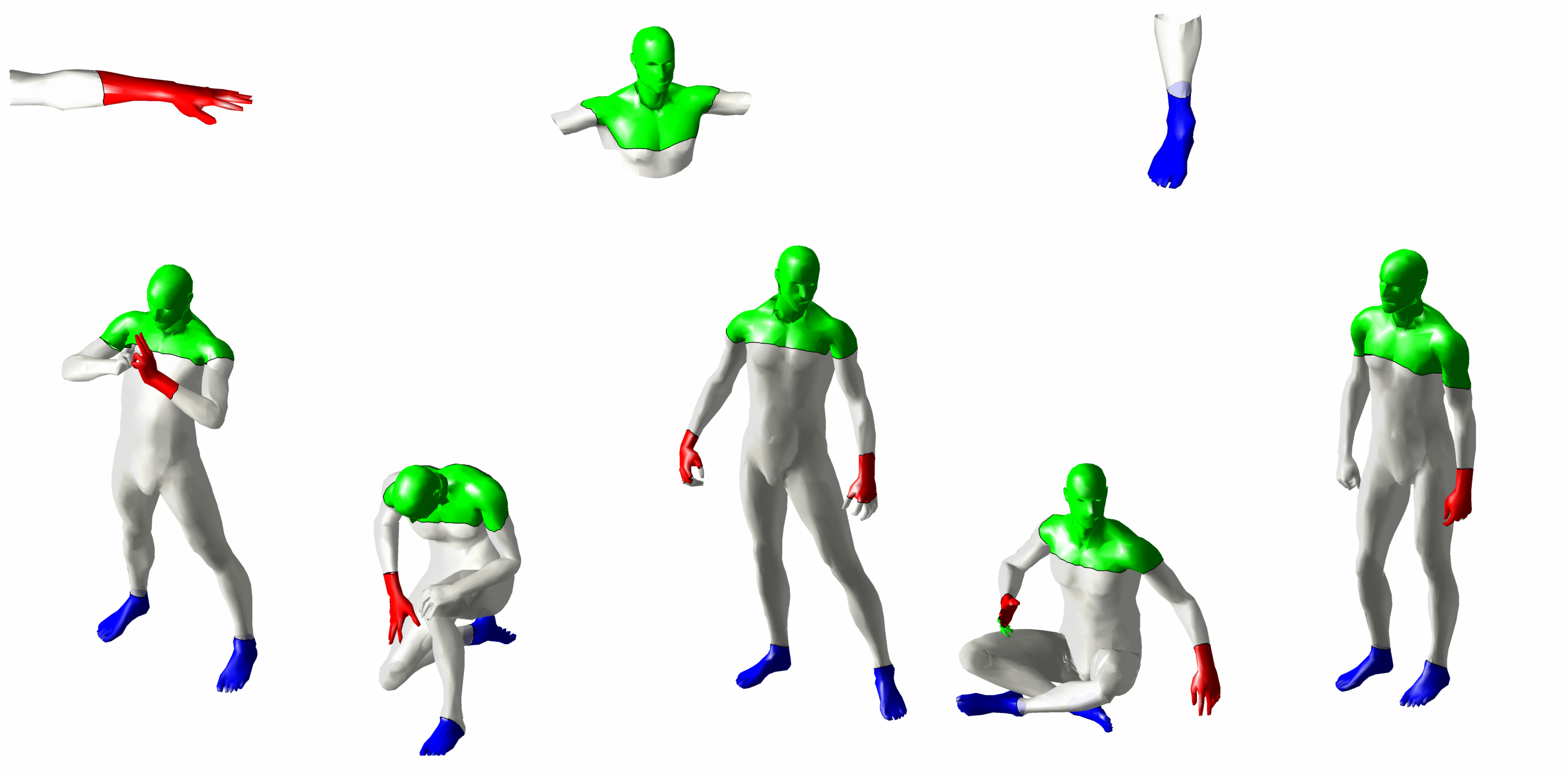
In order to test our approach, we performed several partial matching experiments on data from the SHREC 2010 benchmark [8, 7] and the TOSCA dataset [6].¹¹ 1 Both datasets are available online at http://tosca.cs.technion.ac.il The datasets contained high-resolution (10K-50K vertices) triangular meshes of human and animal shapes with simulated transformations, with known groundtruth correspondence between the transformed shapes. In our experiments, all the shapes were downsampled to approximately 2500 vertices. Parts were cut by taking a geodesic circle of random radius around a random center point.

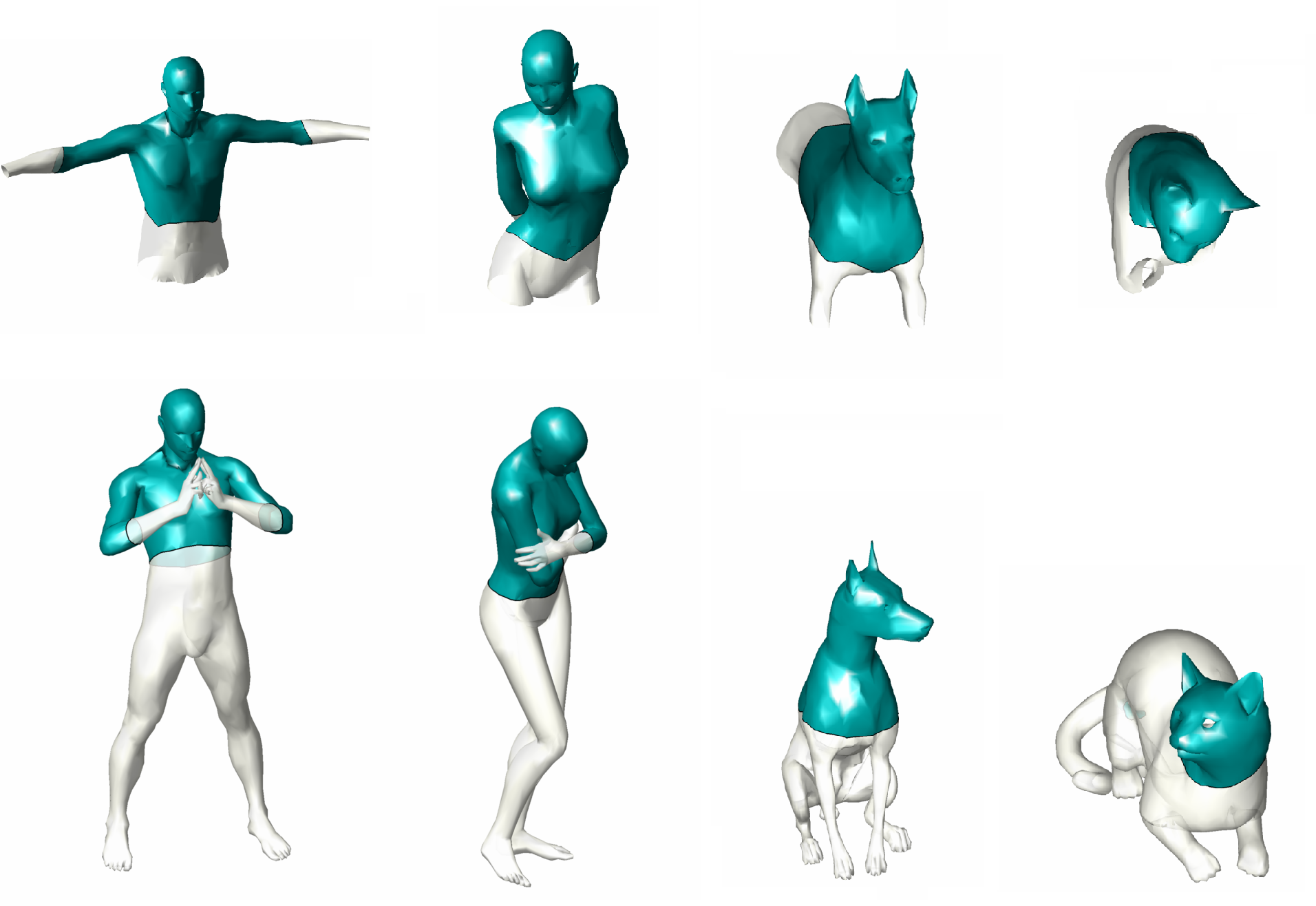
For each part, the normalized HKS descriptor was calculated at each vertex belonging to the part. To avoid boundary effects (see Figure 1), descriptors close to the boundary were ignored when calculating $\overline{\bm{\mathrm{q}}}$ in (4). The distance from the boundary was selected in accordance to the time scales of the HKS. We used ten linearly spread samples in range $[65,90]$ for the descriptors and the according distance taken from edge was set to $15$. Two to three iterations of the alternating minimization procedure were used, exhibiting fast convergence (Figure 3). After three iterations the member function $\bm{\mathrm{u}}$ typically ceased changing significantly. The phase map $\rho$ assumed the values close to $1$ in places of low gradient of the membership function $\bm{\mathrm{u}}$, and less than $1$ in high gradient areas (Figure 3). The importance of the regularization step is is evident observing the change in $\bm{\mathrm{u}}$ in Figure 3. Figure 3 shows the influence of the parameter $\lambda_{\mathrm{r}}$, controlling the impact of the regularization. For too small values of $\lambda_{\mathrm{r}}$, two equally weighted matches are obtained due to symmetry (left). The phenomenon decreases with the increase of the influence of the regularization penalty. However, increasing $\lambda_{\mathrm{r}}$ more causes incorrect matching (second and third columns from the right) due to low data term influence. Increasing it even more starts smoothing the result (rightmost column) until eventually making the membership function uniform over the entire shape. The resulting membership function $\bm{\mathrm{u}}$ was thresholded in such a way that the outcome area will be as close as possible to the query area. Figures 6–6 show examples of matching results after thresholding. Notice that in Figure 6 the matching result sometimes contain the symmetric counter part of the result due to invariance of the HKS descriptor to intrinsic symmetry. (in this figure, the threshold was adjusted to the value of $0.35$ when the membership functions weights are split between two symmetric parts as in Figure  3). The method is robust to shape deformations and geometric and topological noise as depicted in Figure 6. Note that the figures show part-to-whole shape matching, but because of the low scale HKS descriptors the same procedure works for matching to other parts as well.

Table 1 summarizes quantitative evaluation that was performed on a subset of the SHREC database, for which groundtruth correspondence and its bilaterally symmetric counterpart were available. This subset included a male, a dog and a horse shape classes with different geometric, topological and noise deformations ($98$ shapes in total). The query set was generated by selecting a part from a deformed shape ($1000$ queries in each deformation category) and matched to the null shape with parameters and thresholds as described above.

We presented a framework for finding partial similarity between shapes which does not rely on explicit correspondence. The method is based on regularized matching of region-wise local descriptors, and can be efficiently implemented. Experimental results show that our approach performs well in challenging matching scenarios, such as the presence of geometric and topological noise. In the future work, we will extend the method to the setting of two partially-similar full shapes, in which two similar parts have to be found in each shape, and then consider a multi-part matching (puzzle) scenario.

References

- [1] L. Ambrosio and V.M. Tortorelli. Approximation of functionals depending on jumps by elliptic functionals via-convergence. Comm. Pure Appl. Math, 43(8):999–1036, 1990.
- [2] A. M. Bronstein and M. M. Bronstein. Not only size matters: regularized partial matching of nonrigid shapes. In Prof. NORDIA, 2008.
- [3] A. M. Bronstein and M. M. Bronstein. Regularized partial matching of rigid shapes. In Proc. ECCV, pages 143–154, 2008.
- [4] A. M. Bronstein, M. M. Bronstein, A. M. Bruckstein, and R. Kimmel. Partial similarity of objects, or how to compare a centaur to a horse. IJCV, 84(2):163–183, 2009.
- [5] A. M. Bronstein, M. M. Bronstein, and R. Kimmel. Generalized multidimensional scaling: a framework for isometry-invariant partial surface matching. Proc. National Academy of Science (PNAS), 103(5):1168–1172, 2006.
- [6] A. M. Bronstein, M. M. Bronstein, and R. Kimmel. Numerical geometry of non-rigid shapes. Springer-Verlag New York Inc, 2008.
- [7] AM Bronstein, MM Bronstein, B. Bustos, U. Castellani, M. Crisani, B. Falcidieno, LJ Guibas, I. Kokkinos, V. Murino, M. Ovsjanikov, et al. SHREC 2010: robust feature detection and description benchmark. Proc. 3DOR, 2010.
- [8] AM Bronstein, MM Bronstein, U. Castellani, A. Dubrovina, LJ Guibas, RP Horaud, R. Kimmel, D. Knossow, E. von Lavante, D. Mateus, et al. SHREC 2010: robust correspondence benchmark. In Eurographics Workshop on 3D Object Retrieval, 2010.
- [9] M. M. Bronstein and I. Kokkinos. Scale-invariant heat kernel signatures for non-rigid shape recognition. In Proc. CVPR, 2010.
- [10] T. F. Chan and L. A. Vese. Active contours without edges. IEEE Trans. Image Processing, 10(2):266–277, 2001.
- [11] U. Clarenz, M. Rumpf, and A. Telea. Robust feature detection and local classification for surfaces based on moment analysis. Trans. Visualization and Computer Graphics, 10(5):516–524, 2004.
- [12] C. Domokos and Z. Kato. Affine Puzzle: Realigning Deformed Object Fragments without Correspondences. In Proc. ECCV, pages 777–790, 2010.
- [13] M.S. Floater and K. Hormann. Surface parameterization: a tutorial and survey. Advances in Multiresolution for Geometric Modelling, 1, 2005.
- [14] M. Gromov. Structures Métriques Pour les Variétés Riemanniennes. Number 1 in Textes Mathématiques. 1981.
- [15] D. Jacobs, D. Weinshall, and Y. Gdalyahu. Class representation and image retrieval with non-metric distances. Trans. PAMI, 22(6):583–600, 2000.
- [16] A. E. Johnson and M. Hebert. Using spin images for efficient object recognition in cluttered 3D scenes. Trans. PAMI, 21(5):433–449, 1999.
- [17] B. Lévy. Laplace-Beltrami eigenfunctions towards an algorithm that “understands” geometry. In Proc. Shape Modeling and Applications, 2006.
- [18] S. Manay, B.W. Hong, A.J. Yezzi, and S. Soatto. Integral invariant signatures. Lecture Notes in Computer Science, pages 87–99, 2004.
- [19] F. Mémoli and G. Sapiro. A theoretical and computational framework for isometry invariant recognition of point cloud data. Foundations of Computational Mathematics, 5:313–346, 2005.
- [20] M. Meyer, M. Desbrun, P. Schroder, and A. H. Barr. Discrete differential-geometry operators for triangulated 2-manifolds. Visualization and Mathematics III, pages 35–57, 2003.
- [21] N. J. Mitra, L. J. Guibas, J. Giesen, and M. Pauly. Probabilistic fingerprints for shapes. In Proc. SGP, 2006.
- [22] D. Mumford and J. Shah. Optimal approximations by piecewise smooth functions and associated variational problems. Communications on pure and applied mathematics, 42(5):577–685, 1989.
- [23] M. Ovsjanikov, A.M. Bronstein, L.J. Guibas, and M.M. Bronstein. Shape Google: a computer vision approach to invariant shape retrieval. In Proc. NORDIA. Citeseer, 2009.
- [24] M. Pauly, R. Keiser, and M. Gross. Multi-scale feature extraction on point-sampled surfaces. In Computer Graphics Forum, volume 22, pages 281–289, 2003.
- [25] U. Pinkall and K. Polthier. Computing discrete minimal surfaces and their conjugates. Experimental mathematics, 2(1):15–36, 1993.
- [26] Martin Reuter, Franz-Erich Wolter, and Niklas Peinecke. Laplace-spectra as fingerprints for shape matching. In Proc. ACM Symp. Solid and Physical Modeling, pages 101–106, 2005.
- [27] I. Sipiran and B. Bustos. A robust 3D interest points detector based on Harris operator. In Proc. 3DOR, pages 7–14. Eurographics, 2010.
- [28] J. Sivic and A. Zisserman. Video Google: a text retrieval approach to object matching in videos. In Proc. CVPR, 2003.
- [29] J. Sun, M. Ovsjanikov, and L. Guibas. A Concise and Provably Informative Multi-Scale Signature Based on Heat Diffusion. In Computer Graphics Forum, volume 28, pages 1383–1392, 2009.
- [30] R. Toldo, U. Castellani, and A. Fusiello. Visual vocabulary signature for 3D object retrieval and partial matching. In Proc. 3DOR, 2009.
- [31] M. Wardetzky, S. Mathur, F. Kälberer, and E. Grinspun. Discrete Laplace operators: no free lunch. In Conf. Computer Graphics and Interactive Techniques, 2008.
- [32] A. Zaharescu, E. Boyer, K. Varanasi, and R Horaud. Surface feature detection and description with applications to mesh matching. In Proc. CVPR, 2009.
- [33] C. Zhang and T. Chen. Efficient feature extraction for 2D/3D objects in mesh representation. In Proc. ICIP, volume 3, 2001.