UCSD PTH/11-01
Ultraviolet Properties of the Higgs Sector
in the Lee-Wick Standard Model
José R. Espinosaa and Benjamín
Grinsteinb
aICREA, Instituciò Catalana de Recerca i Estudis Avançats,
Barcelona, Spain
at IFAE, Universitat Autònoma de Barcelona, 08193 Bellaterra, Barcelona, Spain
bDepartment of Physics, University of California, San Diego, CA 92093 USA
Abstract
The Lee-Wick (LW) Standard Model (SM) offers a new solution to the hierarchy problem. We discuss, using effective potential techniques, its peculiar ultraviolet (UV) behaviour. We show how quadratic divergences in the Higgs mass cancel as a result of the unusual dependence of LW fields on the Higgs background (in a manner reminiscent of Little Higgses). We then extract from the effective potential the renormalization group evolution of the Higgs quartic coupling above the LW scale. After clarifying an apparent discrepancy with previous results for the LW Abelian Higgs model we focus on the LWSM. In contrast with the SM case, for any , grows monotonically and hits a Landau pole at a fixed trans-Planckian scale (never turning negative in the UV). Then, the perturbativity and stability bounds on disappear. We identify a cutoff GeV for the LWSM due to the hypercharge gauge coupling hitting a Landau pole. Finally, we also discuss briefly the possible impact of the UV properties of the LW models on their behaviour at finite temperature, in particular regarding symmetry nonrestoration.
1 Introduction
In an effort to tame the divergences of quantum field theory Dirac proposed a formulation of quantum mechanics with indefinite metric in the Hilbert space [1]. Pauli further studied Dirac’s proposal and found it to be effective in eliminating certain divergences but failed to give a consistent interpretation of the theory [2]. Pauli and Villars showed that Lagrangians with derivatives higher than of the second order are equivalent to negative metric theories without higher derivatives [3]. They introduced the now famous regulator procedure in which the negative metric states are rendered arbitrarily heavy at the end of the computation. Two decades later, motivated by their desire to eliminate infinities in QED, Lee and Wick (LW) proposed a solution to the question of interpretation of negative metric quantization [4]. They argued that under certain conditions a theory of this kind has a unitary -matrix. Physically their proposal is that states that in the absence of interactions are of negative metric may well be unstable when interactions are present and sufficiently strong. Since unstable states are not asymptotic, only the subspace of the Hilbert space corresponding to positive metric contributes to the -matrix.
The work of ’t Hooft and Veltman on renormalization of gauge theories shelved the LW proposal for a decade, but it was dusted with growing interest in quantizing gravity. In particular it was shown that a higher derivative version of Einstein’s theory of relativity is renormalizable [5] and asymptotically free [6]. More recently it was realized that the Higgs mass in higher derivative versions of the Standard Model (SM) of electroweak interactions does not suffer from a quadratic divergence [7]. Instead there is only logarithmic sensitivity to the cut-off, and the shift in the Higgs mass is of order , where is the scale that characterizes the higher derivatives. The result remains valid even if the model is extended to incorporate right handed neutrinos with masses much large than , that generate light Majorana masses via the see-saw mechanism [8].
This “Lee-Wick Standard Model” (LWSM) is consistent with electroweak precision data [9] and with flavor physics constraints provided is at least a few TeV [10]. The electroweak data favors a light Higgs, – 200 GeV, which remarkably requires little if any finetuning for a few TeV. Such low values for have observable effects in collider experiments. At the LHC one would expect to see resonances [11] associated with would-be negative metric states, roughly one per SM particle.
While this successful yet natural phenomenology is encouraging, there remain many questions of principle with regard to the Lee-Wick proposal. Whether the LW proposal yields a unitary theory is unknown in general. Cutkosky, Landshoff, Olive and Polkinghorne sharpened the prescription of Lee and Wick and showed that large classes of diagrams in perturbation theory satisfy the cutting relations needed for perturbative unitarity [12]. Yet, for some specific models unitarity can be shown to hold explicitly to all orders [13, 14]. Boulware and Gross have identified difficulties with a path integral formulation of the theory [15], but van Tonder has recently proposed a non-perturbative definition for the theory [16]. And, already known to Lee and Wick, their quantization procedure gives non-local correlations that are readily interpreted as non-causal effects.
These non-causality is readily seen as time advancement in certain scattering processes. To be sure, in the LWSM, with the scale of order of a few TeV, these time advancements are unmeasurably short at present. A question immediately arises as to whether a macroscopic sequence of non-causal effects could be contrived to produce macroscopic violations of cause and effect, rendering these theories inconsistent. Coleman argued that this is not possible, but gave no detailed argument [17]. An attempt to address this question indirectly was made in Ref. [18], where the behavior of LW models at high temperature was studied. The speed of sound was found to increase with temperature but never to exceed the speed of light. However, a somewhat surprising and discouraging effect was discovered. The energy density of a LW gas of fermions was determined to decrease without bound as the temperature is increased.
Intending to throw some light into this problem we propose as a first step to investigate the effective potential of LW theories with scalars, fermions and gauge bosons. In Sec. 2 we examine the UV behaviour of the Coleman-Weinberg effective potential in such generic LW theories, using for simplicity the higher-derivative formulation and Landau gauge (discussing in turn the contributions to the potential of generic bosonic and fermionic degrees of freedom). In order to show the cancellation of some UV divergences, we find convenient to regularize the potential using a momentum cutoff. Similarities between Lee-Wick and Little-Higgs theories show up most clearly in this language. We also investigate the finite part of the potential and ask, for example, under what conditions it may have runaway directions.
As a by-product, from the effective potential we are able to determine some renormalization group equations (RGEs) in specific models: making use of the renormalization-scale independence of the effective potential (and the knowledge of the scalar anomalous dimension) it is possible to extract from the one-loop effective potential the RGEs of the parameters of the tree level potential (mass terms and quartic coupling). RGEs for Yang-Mills LW models with fermions and scalars were determined in Ref. [19]. The models did not include scalar self-couplings and the calculations were performed in Landau gauge. The LW Abelian-Higgs model for arbitrary -gauge, including a scalar self-coupling was computed in Ref. [20] with the surprising result that the beta function of the scalar self-coupling vanishes. Our computation of the effective potential gives results at odds with Ref. [20]. In particular, we find that the quartic self-coupling does run. To fully clarify and settle this issue, we present four independent calculations of the RGEs of the model, to wit, by computing green functions diagrammatically (Sec. 3) or by computing the effective potential (Sec. 4), and in both cases in the higher derivative and auxiliary-field formulations. To show explicitly that calculations in different formulations agree requires matching correctly the parameters of both formulations and dealing with a subtlety in the treatment of anomalous dimensions in the auxiliary-field formulation of the model. In the end, the discrepancy with [20] is only apparent and due to a different renormalization prescription.
Finally, Sec. 5 discusses the implications of the softer UV behaviour of the LW scalar sector in the context of the LW Standard Model. First, we derive in Sec. 5.1 the RGEs of the parameters of the Higgs sector in the LWSM, with particular attention to the Higgs quartic coupling. We find that the running of this coupling is better UV-behaved than in the normal SM: it does not get driven to negative values at high energy if the Higgs mass is low nor does it blow-up below the Planck mass if the Higgs mass is large. As a result, in the LWSM the lower stability bound and the perturbativity bound on the Higgs mass disappear. Nevertheless, the RG evolution of gauge couplings above the LW mass scale is also modified [19] and we find a Landau pole for the gauge coupling at a scale GeV (for TeV). This implies that the pure LWSM cannot be extrapolated up to the Planck scale and new physics should appear at or below .
At finite temperature (Sec. 5.2) there is another reason why the ultraviolet behavior of the LW effective potential is of interest. In Little Higgs models EW symmetry can remain broken at high temperature. More generally, symmetry non-restoration can occur in models for which quadratic divergences in the Higgs mass cancel among states with same statistics [21]. Heuristically, this is because corrections to the finite temperature effective potential, which are responsible for symmetry restoration, are directly related to quadratic divergences to the Higgs mass at zero temperature. Since in LW theories cancellation of divergences are among states with same statistics we should then find that EW symmetry might not get restored at high temperature. However, it is not immediately obvious how to extend the standard calculation of the finite temperature effective potential to LW models. At any rate, the above argument indicates that the fate of symmetry at high temperature is determined by the sensitivity of the effective potential to the ultraviolet.
2 Structure of the LW Effective Potential
In order to compute the effective potential in LW theories, we choose to do the computation using a simple momentum cutoff to regularize divergent integrals. This makes the UV behavior, in particular the absence of quadratic divergences, more readily apparent.
2.1 UV Behaviour of the Effective Potential
As preparation for the computation in LW theories, let us begin by revisiting the normal (non-LW) case. Consider a theory of a single self-interacting scalar,
| (1) |
with a SM-like Higgs sector with tree-level potential
| (2) |
In the presence of a uniform background, , the one-loop vacuum diagrams are each infrared divergent. The divergence is, however, an artifact of perturbation theory and the IR finite sum gives the effective potential:
| (3) |
Here is the mass in the non-vanishing uniform background. The result is readily generalized to theories of many fields, including scalars, fermions and gauge bosons:
| (4) |
where the sum is over particle species with degrees of freedom (negative for fermions) and mass (dependent in general on the Higgs field background) and is the Euclidian momentum.
Although one could integrate (3) exactly, we can readily extract the dominant UV behaviour simply by taking the derivative of with respect to , doing the momentum integral and then integrating in . In this way, one gets
| (5) |
where the dots stand for finite terms or terms suppressed by inverse powers of the cutoff. We have used the super-trace, Str, to denote the trace of a matrix weighted by the number of degrees of freedom, and stands for a matrix of masses of all fields in the background of the Higgs fields. As usual, the logarithmic dependence on the cutoff tracks the RG evolution of the parameters of the model. In section 4 we will use effective potential expressions like these to derive RGEs in LW models.
2.2 Bosonic Contributions to the LW Effective Potential
We now turn to the case of LW theories. Take for definiteness the case of scalar fields. The Lagrangian is now
| (6) |
The Feynman rules now have quadratic polynomials in in propagator denominators. Repeating the steps that lead to Eq. (3) one finds instead:
| (7) |
The Wick-rotation to Euclidean momentum is justified by the Lee-Wick prescription for the contour of integration in the complex energy plane. That is, first, in the theory with interactions switched off, take the usual Feynman contour, just above or below the real axis as determined by the prescription. Then deform it to avoid crossing the poles that migrate into the complex energy plane as the interactions in the LW model are switched on.
This generic form is also applicable to gauge bosons in Landau gauge. In LW theory, for each gauge field, supplement the Lagrangian with a term . In a later section we discuss the more general case with a renormalizable gauge-fixing. The main points presented in this section are not affected by sticking to the simpler Landau gauge.
Just as above, the integral is most easily performed by differentiating and integrating with respect to masses. One gets the following UV behaviour
| (8) |
Comparing with (5), we immediately see striking dissimilarities: there is no quadratic divergence and the structure of the logarithmic divergence is quite different. The latter has the structure of the quadratic divergence of the normal case if were the cutoff. This is expected since in a scalar theory the higher derivatives could be used as a regulator.
In order to better understand this result it is useful to look at the LW theory in terms of new auxiliary LW degrees of freedom added to a standard theory. In this formulation terms higher than quadratic in derivatives are absent from the Lagrangian. Instead, these extra LW fields are responsible for the additional poles of the modified propagator. That is, the masses of the normal and auxiliary LW fields correspond to the solutions of the pole equation:
| (9) |
and the LW field is identified by the pole with negative residue. This corresponds to a wrong sign kinetic energy term in the Lagrangian. Alternatively one can make the sign of the kinetic term of the auxiliary LW field standard by rescaling the field by . Then the structure of these pole masses can also be obtained as coming from a non-hermitian mass matrix of the form
| (10) |
The two solutions of the pole equation (9), or, equivalently, the two eingenvalues of the mass matrix (10), are
| (11) |
These two masses are real if . This holds for the usual choice of parameters in applications of LW theory to the hierarchy problem since are of electroweak size while is taken in the several TeV range. When calculating the one-loop effective potential for values of the Higgs field background for which , the two masses (11) are complex conjugate pairs, their sum giving a real contribution to the potential (see below). Expanding the masses (11) in powers of we find
| (12) | ||||

Figure 1 shows the squared-masses for bosons throughout both low and high Higgs background regions as a function of the ratio . The two complex masses in the high region are represented by plotting their real part, , as a solid line while the dashed lines give as a convenient way of plotting the information on the imaginary parts.
In summary, for each standard bosonic degree of freedom with mass squared (up to corrections suppressed by ) there is a new LW degree of freedom with mass squared completing a “LW-multiplet.” Using the standard formula (5) for these degrees of freedom and keeping a unique label for each SM-LW pair we reproduce the UV behaviour of (8), up to an irrelevant background-field independent constant. One sees explicitly that this is the result of cancellations between the normal and LW contributions. We can also see this cancellation as occurring through and directly without any power expansion, which is one of the uses of writing down the mass matrix in (10). One can also see the two contributions arising directly from the integral (7) by factoring the argument of the logarithm:
| (13) |
Explicitly, the contribution to the one-loop potential reads
| (14) |
where we have merely used the standard Coleman-Weinberg expression in Landau gauge. Here for gauge bosons, for scalars and is the renormalization scale.
In the low field region, for which , the potential above takes the form
| (15) |
with
| (16) |
By contrast, in the high field region, for which , the potential above takes the form11 1 Note that (15) is simply the analytic continuation of (17) into .
| (17) |
with
| (18) |
We can see from this result that the bosonic contributions to the one-loop effective potential now grow only like for high (to be compared with the growth in the normal case). Therefore, in that region of field space the tree level term will dominate.
2.3 Fermionic Contributions to the LW Effective Potential
We consider next the contributions of fermions to the effective potential in a theory with higher derivatives. The terms in the Lagrangian with derivatives on fermions are
| (19) |
The fermionic contributions to the effective potential in LW theories can be obtained through an analysis similar to the one for bosons above. Instead of (3), for fermions in LW theories one has
| (20) |
where, we remind the reader, we have included a minus sign in . By applying the same procedure as above one finds that fermions do not contribute to the potential a field-dependent UV divergence, not even logarithmic.
Again, we can understand this result in terms of new auxiliary LW fermionic degrees of freedom. Now, the equation giving the propagator poles reads
| (21) |
where is the mass of the standard fermionic degree of freedom. This pole equation admits now two additional solutions, corresponding to two additional LW degrees of freedom. The structure of these pole masses can be obtained in an equivalent manner as coming from a non-hermitian mass-squared matrix of the form22 2 We are assuming that both LW fields appear with the same heavy mass for simplicity, but this is not necessary. In the most general case the LW mass in the 33 entry in (22) can be different from the other LW mass.
| (22) |
which is what one would obtain by rescaling the auxiliary LW fields by and , which gives a standard sign for their kinetic term.
The eigenvalues of this matrix, or the solutions to the pole equation, Eq. (21), are
where the angle is given by
| (23) |
We assume here that , which guarantees real masses. An expansion in powers of gives
| (24) | ||||
Therefore, each standard fermionic degree of freedom is accompanied by two quasidegenerate heavy LW-fields completing a fermionic “LW-multiplet.”
Using the standard formula (5) for the contribution of these degrees of freedom to the one-loop potential and keeping a unique label for each standard-LW fermionic multiplet, we reproduce (up to a field-independent constant) the UV finiteness of Eq. (20) as a result of standard-LW cancellations. The same cancellations can be seen as operating directly in and for the fermionic mass matrix (22). At the level of the integral (20) the three separate contributions to the effective potential follow simply from writing the argument of the logarithm in factorized form:
| (25) |
The explicit expression for the potential is
| (26) |
where now . In fact, the only dependence on that appears in (26) affects the renormalization of a background-field independent term. For the purpose of studying the shape of the background-field dependent potential, we can therefore simply drop and altogether in that expression.
In the high-field region, for which , one of the three mass eigenvalues is still real while the other two form a complex conjugate pair. They are
| (27) | ||||
where we have used the functions
| (28) |
For later use, we quote the useful relation .

In the high field region, , the effective potential takes the form:
| (29) |
where
| (30) | ||||
that is, . Different fermionic contributions in Eq. (29) grow at high as and . There is a cancellation of the dominant terms, leaving a total result that grows only as . These contributions are therefore subdominant compared with the tree-level quartic.
Figure 2 shows the squared-masses for fermions throughout both low and high background field regions as a function of the ratio . The complex masses in the high region are represented by plotting as a solid line and as dashed lines.
3 RGEs in the LW Abelian Higgs Model. Diagrammatic Approach
As a warm-up for the LWSM case, in this section we calculate the renormalization group equations (RGEs) of the scalar sector parameters in the Lee-Wick Abelian Higgs model. We do this by computing directly the one-loop counterterms needed to renormalize Green functions. We compute them first, in Sec. 3.1, using the higher-derivative formulation of the model and then we calculate them again, in Sec. 3.2, using the auxiliary-field formulation. We find agreement between both approaches, once the parameters in the two formulations are appropriately matched to each other. These results will be used as the benchmark against which the effective potential calculation of the RGEs (Sec. 4) can be compared. This model already captures the main features and subtleties of the LWSM calculation (which we present in section 5) with the advantage of being simpler.
3.1 Diagrammatic Approach in the Higher-Derivative Formulation
The Lagrangian of the LW Abelian Higgs model in the higher-derivative formulation (indicated by hatted fields and parameters) reads:
| (31) |
where and we show explicitly the gauge-fixing term. With this gauge-fixing the gauge-boson propagator is
| (32) |
The scalar propagator can be written as
| (33) |
with and .
We are interested in calculating the RGEs of the parameters in the scalar sector of the theory, that is, the beta functions of , , and the anomalous dimension of . A straightforward one-loop diagrammatic calculation using dimensional regularization gives the following result for the divergent piece of the scalar two-point function:
| (34) |
where
| (35) |
with and the Euler constant. From Eq. (34) we can extract in the standard way the following RGEs:
| (36) | ||||
| (37) | ||||
| (38) |
At and these results are in accord with Ref. [19].
In order to get the RGE for the scalar quartic coupling we need the divergent part of the four-point scalar function. In the limit of vanishing external momenta tending to zero, it reads
| (39) |
where is normalized as . Note that there are no contributions of order (the corresponding diagrams are finite) or (UV divergences of separate diagrams cancel out). From Eq. (39) and the previous result on the scalar anomalous dimension, Eq. (36), we obtain
| (40) |
This completes our task. As expected on general grounds [22], the one-loop beta functions for , and are gauge independent and only the scalar anomalous dimension depends on the gauge-fixing parameter .
3.2 Diagrammatic Approach in the Auxiliary-Field Formulation
We now turn to the calculation of the RGEs in the auxiliary-field formulation, with derivatives at most of second order. We need an auxiliary-field Lagrangian equivalent to the Higher derivative one in Eq. (31), which we can get by adding auxiliary fields through
| (41) |
where is the higher-derivative Lagrangian in Eq. (31). Replacing the field through the change of variables and performing a symplectic rotation
| (42) |
with
| (43) |
we obtain
| (44) |
where now .
The dictionary between the new parameters , , and appearing in Eq. (44) and the original parameters in is the following:
| (45) | ||||
and the trivial equality . The inverse relations are:
| (46) | ||||
Note that and correspond to the pole masses and of the higher-derivative scalar propagator, as given by Eq. (33).
Before we compute directly the RGE for the parameters of this model (, and ) we can obtain them indirectly by differentiating relations (45) and using the corresponding RGEs for the hatted parameters, calculated in the preceding subsection, and then use the relations (46) to express the results in terms of unhatted parameters. In this way one arrives at
| (47) | ||||
| (48) | ||||
| (49) |
We now proceed to verify that these results follow from direct diagrammatic calculation in the auxiliary-field formulation. Explicitly, the divergent part of the two-point functions are:
| (50) | ||||
These divergences can be compensated by counterterms in the usual way. Although the renormalization of the kinetic terms is invariant under an rotation among the fields and , as explained in [20], such rotation introduces mixed mass terms. For this reason we can absorb the non-zero , which requires a mixed - counterterm, through an off-diagonal anomalous dimension (even if the divergence is momentum-independent).33 3 Alternatively, one could introduce a new mass term in the potential, , but this can always be rotated away by a field redefinition. Our prescription can be reinterpreted in terms of a renormalization of the mixing angle . More explicitly, we obtain
| (51) |
These anomalous dimensions reproduce of Eq. (36), as can be easily checked simply writing in terms of and . With the use of these anomalous dimensions we can also obtain the RGEs for and from Eqs. (50) obtaining precisely the results anticipated by Eqs. (47) and (48).
In order to get the one-loop RGE for it is enough to compute the divergent part of the one-loop four-point function for . In the limit of vanishing external momentum we obtain
| (52) |
where is normalized as . The divergent pieces of mixed - four-point functions are such that is the divergent operator in the one-loop effective action, so that a single counterterm for can absorb that divergence. Making use of the scalar anomalous dimensions as given by Eqs. (51) one obtains a beta function for that reproduces the result given in Eq. (49).
In Ref. [20] a different result is found, namely . This is the result of renormalizing differently the scalar mass terms and wave-functions, along the lines of footnote 3. Using such prescription implies in particular that the Higgs quartic coupling in [20] differs from ours by an overall factor (that depends on the field-mixing radiatively induced) and therefore runs differently. While the prescription in [20] is simpler in the sense of having a non-running , it requires the introduction of an additional mass parameter, which is absent in our prescription. Needless to say, all physical predictions of the theory should be prescription-independent.
4 RGEs in the LW Abelian Higgs Model. Effective Potential Approach
In this section we will rederive the RGEs for the parameters of the scalar sector in the LW Abelian Higgs Model via the Coleman-Weinberg potential and the scalar anomalous dimensions of the scalar field(s). The technique, based on the scale-independence of the effective potential, is well known [23]. Consider a model with SM-like tree-level potential
| (53) |
The one-loop Coleman-Weinberg correction is
| (54) |
where the sum runs over species with -dependent mass-squared and degrees of freedom (taken negative for fermions); is the renormalization scale and for gauge bosons (scalars or fermions). Imposing one-loop RG invariance of one obtains the relations
| (55) |
| (56) |
where and , as usual. For masses of the generic form one then obtains
| (57) |
| (58) |
This procedure can be generalized trivially to cases with mass mixing and/or several scalar fields.
In order to determine the beta functions it is necessary to calculate the anomalous dimension(s) separately. For the case of the Abelian Higgs model we will take them from the previous section. (In Sec. 4.2 we will discuss the subtleties that arise due to mixing of the anomalous dimensions of normal and LW scalars in the auxiliary field formalism.)
For the purpose of calculating these beta functions in a given model we do not need to calculate explicitly the ’s because the scale dependence of only involves , see (55) and (56). In general, the ’s in each sector of the theory are solutions, , of polynomial secular equations of the general form:
| (59) |
where the are functions of the background field . Writing formally this equation as
| (60) |
we immediately get
| (61) |
We will use these equations in what follows, applying them sector by sector, to compute the separate contributions to the supertrace .
Before embarking into that detailed calculation for the Abelian Higgs Model, we can apply this technique to a general LW theory in the simple Landau gauge and assuming a unique LW mass (the case considered in our previous analysis of LW effective potential contributions). Bosonic LW multiplets, with pole equation as in (9), will contribute to the piece
| (62) |
while fermionic LW multiplets, with pole equation as in (21), will give the -independent piece
| (63) |
If we input these results in the general formulas (55) and (56) and use we get, instead of the standard RGEs given in Eqs. (57)–(58),
| (64) | |||
| (65) |
where the primed sum indicates that only bosons contribute and labels LW multiplets. In general, the Lee-Wick mass can be different for different scalar fields, in which case the above formula (64) should be generalized in a straightforward way.
4.1 Effective Potential Approach in the Higher-Derivative Formulation
We give a nonzero background value to the complex scalar field and write
| (66) |
and then proceed to derive the (inverse) propagators in that background. The zeros of such inverse propagators will occur at the squared masses . For the scalar field we find the secular equation
| (67) |
with . The inverse propagator for the pseudoscalar field is similarly obtained with but, with the gauge-fixing as in Eq. (31), there is also mixing between and . The inverse propagator for the - sector is the matrix
| (68) |
where . Equating the determinant of this matrix to zero we get the secular equation
| (69) |
for the pole masses in this sector. We see that this equation splits into two separate equations, of which one gives pole mass solutions with multiplicity 3, corresponding to the different polarizations of a massive gauge boson. Applying to the secular equations (67) and (68) the prescription in Eq. (61) we immediately obtain
| (70) |
where the labels indicate (with some abuse of notation) the origin of each contribution. This trace is independent of , as it should be to cancel quadratic divergences in the scalar mass (see discussion in Sec. 2.2). We also obtain
| (71) | ||||
It follows that
| (72) | ||||
| (73) |
in perfect agreement with the results in Sec. 3.1, Eqs. (36)–(38). One can also check that, in Landau gauge () and for , these equations are in agreement with the general formulas (64) and (65).
4.2 Effective Potential Approach in the Auxiliary-Field Formulation
In this formulation we give a background value and write
| (74) |
while
| (75) |
and then proceed to derive the secular equations for the pole masses in the same way as before.
There is mixing among the CP-even scalars and and their inverse propagator is the matrix
| (76) |
where . Equating the determinant of this matrix to zero, we obtain the secular equation
| (77) |
The fields , , and get all mixed in the -background and their inverse propagator is the matrix
| (78) |
where
| (79) | ||||
| (80) |
which leads to the secular equations
| (81) | ||||
Applying again to the secular equations (77) and (81) the prescription in Eq. (61) we immediately obtain
| (82) |
where the labels indicate (again with some abuse of notation) the origin of each contribution. This trace is independent of , as it should be if the quadratic divergences in the scalar mass are to cancel (see discussion in Sec. 2.2). We also obtain
| (83) |
There is now a subtlety when using the scale-independence of the effective potential due to the fact that, even if the field has no background expectation value, its derivative with the renormalization scale, will have a nonzero background value that arises from mixing with the field . That is, from the tree-level potential
| (84) |
we obtain
| (85) |
where and can be read off Eq. (51). Using the previous result for , Eq. (83), which determines the scale-dependence of the one-loop Coleman-Weinberg correction, we arrive at
| (86) | ||||
| (87) |
in perfect agreement with the results presented in Eqs. (47)-(49).
5 Some Implications of the UV Behaviour of the LW Standard Model
5.1 Implications at Zero Temperature
We have seen that the LW effective potential is softer than in standard theories: on the one hand, the bosonic part of the effective potential, Eq. (8), does not contain a term while, on the other hand, the fermionic part, Eq. (20), is finite. The softer UV behaviour has direct implications for the RGEs of the LW theory above the threshold . Using (57) and (58), the RGEs in the SM, using Landau gauge, satisfy
| (88) | ||||
| (89) |
with the normalization of and as in (2); and are the and gauge couplings and is the top Yukawa coupling. The Higgs anomalous dimension is
| (90) |
Below the scale associated with the new LW degrees of freedom these SM RGEs will still be valid.
Above that scale the full LWSM RGEs should be used. In Landau gauge, we can use the same procedure that leads to (64) and (65) to get
| (91) | ||||
| (92) |
The different Lee-Wick masses are the following: is associated with the Higgs, with the gauge boson and with the gauge boson. Much as in SUSY theories we see that is dictated by wave-function renormalization only. In particular the SM top-quark vertex contribution to this beta function [see Eq. (89)] is absent.
We can easily extend the result for the scalar anomalous dimension in the LW Abelian Higgs Model found in a previous section to the Higgs field in the LWSM and its non-Abelian gauge structure, simply replacing in (36) by , where the sum runs over the different gauge groups (labeled by ) and group generators (labeled by ), with gauge coupling constant and the are the group generator matrices in the representation of the Higgs field. We keep explicit the dependence on the different Lee-Wick masses . In contrast with the SM case, this anomalous dimension only gets contributions from gauge loops (and not from fermions). In Landau gauge it reads:
| (93) |
In these formulas for the LWSM RGEs we are implicitly adopting the higher-derivative formulation. Even if one is interested in a simplified case with , this condition is not stable under RG evolution. The RGEs for the Lee-Wick masses are simple to obtain. Following the results of [19], we know that the combinations and are scale-invariant in Landau gauge. Therefore, the running of the gauge Lee-Wick masses is governed by the evolution of the corresponding gauge couplings, which are given explicitly by [19]
| (94) |
For the RGE of we can generalize the Abelian Higgs case in (37) to
| (95) |
which can be readily integrated.
Focusing on the evolution of the Higgs quartic coupling, we find that its scale running in the LWSM above the LW mass is governed by the RGE:
| (96) |
In leading-log approximation44 4 In fact, following [19], we expect that these beta functions will not receive further contributions beyond one loop, with the exception of , which will still be corrected at two-loop order. it is straightforward to integrate this RGE to obtain
| (97) |
where is the common Lee-Wick mass (at the scale ).
One consequence of this scale dependence is that and that the Higgs effective potential in the LWSM (in contrast with the SM case) will not develop pathologies at high scales.
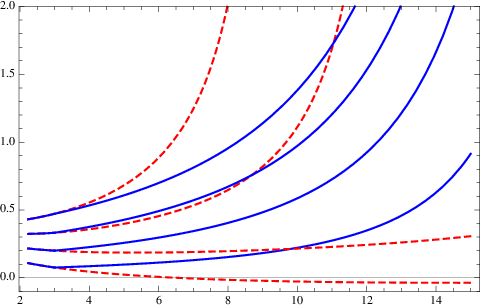
This is shown in Fig. 3, which plots the running (for several Higgs mass choices) in the LW Standard Model (blue solid lines) departing above a Lee-Wick mass TeV from the running in the SM (red dashed lines). The plot shows the well known fact that in the pure SM, if the Higgs is too light, the running turns negative at high energies triggering an instability in the effective potential. Alternatively, if the Higgs is too heavy, runs into a Landau pole below the Planck scale. For the most updated study on this UV fate of the SM and references to the literature, see [24]. In the LW Standard Model, in contrast, the light Higgs instability does not take place (provided the LW mass is below the SM instability scale) because is proportional to itself. On the other hand, the heavy Higgs non-perturbative regime is pushed toward higher masses because does not grow quadratically with as it does in the SM. In fact the explicit solution (97) tells us that hits a Landau pole at
| (98) |
independently of the Higgs mass value. This means in particular that there is no perturbativity bound on the Higgs mass in the LWSM: one could always require , but the obtained bound would not be competitive with the usual unitarity bound, and we do not calculate it.55 5 Lattice studies of such bound in similar models, with a higher-derivative kinetic term as regulator, exist [25] and show a large increase of the bound with respect to the standard case. However, the studied cases use a term, which is higher order than ours, and do not include gauge fields, preventing a direct comparison. Inspection of the beta function for , (95), also shows that at the same scale , which would also be a pathological behaviour. At any rate, the numerical value of this cutoff scale is higher than the Planck mass and is no cause of concern.
In the previous discussion we have used the coupling , from the higher-derivative formulation but similar conclusions follow if we use the auxiliary formulation instead. In that formulation, the RGE for the quartic coupling is now
| (99) |
corresponding to a well-behaved, asymptotically-free coupling. In agreement with the previous results one cannot obtain lower or upper bounds on the Higgs mass on the basis of this running behaviour. Nevertheless, the cutoff scale reappears in this formulation when looking at the running of , which goes to zero at that scale.
On the other hand, the gauge coupling now runs faster than in the SM, see (94), and can become nonperturbative below the Planck mass. The Landau pole for this gauge coupling occurs at
| (100) |
For TeV, one gets GeV. This indicates that new physics beyond the LWSM should appear below . Alternatively, this Landau pole could be pushed beyond the Planck mass if the Lee-Wick mass is higher, but the required value, of order GeV is orders of magnitude too high to solve the hierarchy problem.
5.2 Implications at Finite Temperature
As discussed in the introduction, one possible way of probing the acausal nature of LW theories in search of a macroscopic effect or some pathological behaviour is to study them at finite temperature. The behavior of a LW gas in thermal equilibrium was studied in Ref. [18]. It was found there that the contribution to the free energy of each LW state, that is, of the narrow resonances that would be states of negative metric in the limit that interactions are switched off, is the negative of the contribution of a normal state of the same mass:
| (101) |
Here and and denote volume and temperature. Consider the energy density at high temperature. For each normal scalar degree of freedom (labeled ) giving a normal contribution with mass there is a LW contribution of mass , cf. Eq. (11). A high-temperature expansion shows that each bosonic LW multiplet gives a contribution to the energy density:
| (102) | ||||
where we have assumed and used the mass expansions of Eq. (12) in the last step. Although the normally leading term is missing, the energy density is positive and increases with temperature.
By contrast, the contribution to the energy density of a fermionic LW multiplet includes a normal contribution with mass and two additional contributions from LW modes of masses , cf. Eq. (24), with the opposite sign. The energy density at high temperature is dominated by the term and is given by:
| (103) | ||||
The energy density decreases with temperature and at high enough temperatures turns negative. This peculiar behavior suggests that, either interesting phenomena are taking place in the LW fermionic gas at high temperature or the result (101) is not correct, see below.
We have not computed the effective potential for the scalar field in a plasma at finite temperature. But there is a well known correspondence between the zero temperature self-energy diagrams that exhibit quadratic divergences and the diagrams responsible for a scalar thermal mass [26]. If is a straight momentum cut-off, quadratic divergences in the scalar mass arising from bosonic excitations, , translate into a thermal mass correction . Similarly, for fermionic excitations translate into . Therefore, in models that solve the hierarchy problem by cancellations of the quadratic divergence in the Higgs mass arising from intermediate states of the same spin, one expects a corresponding cancellation in the thermal mass [21].
The cancellation of quadratically-divergent contributions to the scalar potential was shown explicitly in Secs. 2.2 and 2.3 for the bosonic and fermionic cases, respectively. Consider first the bosonic case. The effective potential, given in Eq. (13), is the sum of two same “normal” sign contributions. The mass shift can be obtained by differentiation
| (104) |
where the 0 subscript indicates evaluation at . Since , and is independent of the background field, one has
| (105) |
which shows explicitly the cancellation of quadratic divergences. Rather than performing the angular momentum integral that gives Eq. (13), one can do first the integral over the time component of momentum, yielding
| (106) |
where . The connection with the finite temperature potential is made, at least in the normal case, by replacing the energy integral by a sum over Matsubara modes. Doing this for the LW model, disregarding any subtleties that may arise from the LW and CLOP prescriptions, the finite temperature potential is
| (107) |
Taking a derivative we obtain the mass shift:
| (108) |
Whilst this expression is not fully justified, it does produce the expected results, namely the cut-off independence that takes place as a cancellation of the terms as well as the absence of the thermal mass shift. But, remarkably, it was obtained from an effective potential in which the normal and LW modes enter with normal signs. This is in contrast with the computation of the free energy in Ref. [18] in which the LW modes appear with negative sign. However, we have not been able to find any problem with the derivation in [18] and, at present, we do not know which one of these two results, if either, is correct. LW theory is remarkably intricate and it is possible that missed subtleties have rendered one or the other calculations, or both, incorrect.
The result carries over to the fermionic case. Although there are two LW modes for one normal mode, the sum rule produces the cancellations that are associated with the non-normal signs even though the potential is the sum of normal sign contributions. Therefore if, contrary to the findings of Ref. [18], LW fields contribute to the thermal free-energy with normal signs, one would avoid the problem with a negative fermionic contribution to the energy density discussed before.
We postpone investigation of the properties of this thermal potential until a future time when we understand how to better justify the calculation.
Acknowledgments
The authors would like to thank CERN for hospitality and financial support. The work of J.R.E was supported in part by the European Commission under the European Union through the Marie Curie Research and Training Network “UniverseNet” (MRTN-CT-2006-035863); by the Spanish Consolider-Ingenio 2010 Programme CPAN (CSD2007-00042); and by CICYT, Spain, under contracts FPA 2007-60252 and FPA 2010-17747. The work of B.G. was supported in part by the U.S. Department of Energy under contract DE-FG03-97ER40546.
References
- [1] P. A. M. Dirac, Proc. Roy. Soc. A180 (1942) 1.
- [2] W. Pauli, Revs. Mod. Phys. 15 (1943) 175.
- [3] W. Pauli and F. Villars, Rev. Mod. Phys. 21 (1949) 434.
- [4] T. D. Lee and G. C. Wick, Nucl. Phys. B 9, 209 (1969); Phys. Rev. D 2, 1033 (1970).
- [5] K. S. Stelle, Phys. Rev. D16, 953-969 (1977).
- [6] E. S. Fradkin, A. A. Tseytlin, Phys. Lett. B104, 377-381 (1981); E. S. Fradkin, A. A. Tseytlin, Nucl. Phys. B201, 469-491 (1982).
- [7] B. Grinstein, et. al., Phys. Rev. D 77, 025012 (2008) [hep-ph/0704.1845].
- [8] J. R. Espinosa, et. al., Phys. Rev. D 77, 085002 (2008) [hep-ph/0705.1188].
- [9] T. E. J. Underwood and R. Zwicky, Phys. Rev. D 79, 035016 (2009) [hep-ph/0805.3296]; E. Alvarez,et. al., JHEP 0804, 026 (2008) [hep-ph/0802.1061]; C. D. Carone, R. F. Lebed, Phys. Lett. B668, 221-225 (2008) [hep-ph/0806.4555]; R. S. Chivukula, A. Farzinnia, R. Foadi et al., Phys. Rev. D81, 095015 (2010) [hep-ph/1002.0343].
- [10] T. R. Dulaney and M. B. Wise, Phys. Lett. B 658, 230 (2008) [hep-ph/0708.0567].
- [11] T. G. Rizzo, JHEP 0706, 070 (2007) [hep-ph/0704.3458]; JHEP 0801, 042 (2008) [hep-ph/0712.1791].
- [12] R. E. Cutkosky, et. al., Nucl. Phys. B 12, 281 (1969).
- [13] E. Tomboulis, Phys. Lett. B 70, 361 (1977); Phys. Lett. B 97, 77 (1980); I. Antoniadis and E. Tomboulis, Phys. Rev. D 33, 2756 (1986).
- [14] B. Grinstein et. al. , Phys. Rev. D 79, 105019 (2009) [hep-th/0805.2156].
- [15] D. G. Boulware and D. J. Gross, Nucl. Phys. B 233, 1 (1984).
- [16] A. van Tonder, [hep-th/0810.1928].
- [17] S. Coleman, “Acausality,” In Erice 1969, Ettore Majorana School On Subnuclear Phenomena, A. Zichichi, Editor, Academic Pres, New York, 282 (1970).
- [18] B. Fornal, B. Grinstein, M. B. Wise, Phys. Lett. B674, 330-335 (2009) [hep-th/0902.1585].
- [19] B. Grinstein and D. O’Connell, Phys. Rev. D 78, 105005 (2008) [hep-ph/0801.4034].
- [20] R. S. Chivukula, A. Farzinnia, R. Foadi et al., Phys. Rev. D82, 035015 (2010) [hep-ph/1006.2800].
- [21] J. R. Espinosa, M. Losada, A. Riotto, Phys. Rev. D72, 043520 (2005) [hep-ph/0409070].
- [22] D. J. Gross and F. Wilczek, Phys. Rev. D 8 (1973) 3633.
- [23] See e.g. C. Ford, D. R. T. Jones, P. W. Stephenson and M. B. Einhorn, Nucl. Phys. B 395 (1993) 17 [hep-lat/9210033].
- [24] J. Ellis, J. R. Espinosa, G. F. Giudice, A. Hoecker and A. Riotto, Phys. Lett. B 679 (2009) 369 [hep-ph/0906.0954].
- [25] K. Jansen, J. Kuti and C. Liu, Nucl. Phys. Proc. Suppl. 30 (1993) 681; Phys. Lett. B 309 (1993) 127 [hep-lat/9305004].
- [26] D. Comelli, J. R. Espinosa, Phys. Rev. D55, 6253-6263 (1997) [hep-ph/9606438].