跳到论文正文
W Papers独立论文阅读器 arXiv:1101.5409 论文正文 计算阅读时间 · 0%
引用这篇论文根据当前论文元数据生成,正式投稿前建议核对。


License: arXiv.org perpetual non-exclusive license
arXiv:1101.5409v2 [hep-th] 07 Mar 2011

The Casimir Effect for Conical Pistons

Guglielmo Fucci and Klaus Kirsten ††thanks: Electronic address: gfucci@nmt.edu Note: Electronic address: Guglielmo_Fucci@Baylor.edu Note: Electronic address: Klaus_Kirsten@Baylor.edu Affiliation: Department of Mathematics, Baylor University, Waco, TX 76798 USA
August 24, 2026
Abstract

In this paper we utilize ζ\zeta-function regularization techniques in order to compute the Casimir force for massless scalar fields subject to Dirichlet and Neumann boundary conditions in the setting of the conical piston. The piston geometry is obtained by dividing the bounded generalized cone into two regions separated by its cross section positioned at aa with a∈(0,b)a\in(0,b) with b>0b>0. We obtain expressions for the Casimir force that are valid in any dimension for both Dirichlet and Neumann boundary conditions in terms of the spectral ζ\zeta-function of the piston. As a particular case, we specify the piston to be a dd-dimensional sphere and present explicit results for d=2,3,4,5d=2,3,4,5.

I Introduction

The Casimir effect is one of the most important macroscopic manifestations of the zero point energy of quantized fields under the influence of external conditions [11, 38] or in spaces with non-trivial topology. In recent years, a vast amount of literature has been produced on the Casimir effect, which was first predicted in the seminal paper [13], especially for its relevance in nanoscale physics [10, 11, 38]. Due to its nature, calculations of the vacuum energy lead to divergencies which need to be regularized and subsequently renormalized. Several regularization methods exist, amongst the most important ones are frequency cutoff, point splitting and zeta function regularization [6, 10, 12, 22, 23, 38]. For many configurations, these techniques yield the same finite renormalized result, however the way divergencies are removed is different in each scheme. The non-uniqueness of the removal procedure raises the question, which of them is the physically best motivated one. Technical and interpretational problems of this nature can actually be avoided if one considers the Casimir effect between separate objects. In this case, the divergent part of the energy (for massless fields) depends on the heat kernel coefficient aD/2a_{D/2} related to the geometry of the objects. These coefficients, in turn, do not depend on the distance between the bodies and, hence, the Casimir force between them is free of divergencies [10]. Belonging to the class of configurations for which the Casimir force has been unambiguously evaluated are pistons of certain types.

These piston configurations, introduced in [14], have become increasingly important because of this fact. A large variety of piston configurations and boundary conditions have been studied throughout the literature, both at zero and at finite temperature. Rectangular Casimir pistons with different types of boundary conditions have been considered, for instance, in [21, 32, 33, 36, 48]. Cylindrical Casimir pistons, instead, have been analyzed in [4, 37, 44]. Higher dimensional Casimir pistons with arbitrary cross sections have been studied in the setting of Kaluza-Klein models in [35, 29]. A generalization of these models for finite temperatures has been obtained, e.g., in [42, 43].

In the literature, Casimir piston configurations have the general geometric structure of a direct product I×N×MI\times N\times M, where II is a closed interval of the real line, NN is either a compact or non-compact manifold, and MM is a compact manifold usually describing the extra-dimensions. Pistons of a different geometric nature, where the local line element contains a warp factor, have been recently considered in the framework of five and higher-dimensional Randall-Sundrum models [17, 26, 41]. Moreover, vacuum polarization effects have been studied for massive fermion fields in the context of the global monopole in [5].

In this paper we will focus our attention on a new type of Casimir piston modeled on a conical manifold. The main difference of this configuration from the previous ones studied in the literature is the presence of a singularity at the origin and the fact that the piston is a curved manifold. As a result, only for particular dimensions the force will be unambiguous. This setup is particularly important in order to study the effects on the piston due to the presence of a geometric singularity. The main physical interest for the study of conical manifolds lies in field theoretical models requiring an orbifold compactification [28, 46]. In fact an orbifold is defined locally by the quotient space of a smooth manifold XX and a discrete isometry group GG. The action of the group on the manifold has, in general, fixed points which are mapped to conical singularities in the quotient space. This is a topic of great interest especially in the ambit of string theory [1].

We will utilize ζ\zeta-function techniques in order to obtain analytic expressions for the Casimir energy of the conical piston. The spectrum of a self-adjoint partial differential operator on compact manifolds is discrete, bounded from below and the eigenvalues λn\lambda_{n} form an increasing sequence. In this case one can define the spectral ζ\zeta-function associated to the operator as

ζ⁡(s)=∑n=1∞λn−s,\zeta(s)=\sum_{n=1}^{\infty}\lambda_{n}^{-s}\;, (1)

which is convergent for ℜ⁡(s)>D/2\Re(s)>D/2, with DD being the dimension of the manifold under consideration. One can analytically continue, in a unique way, ζ⁡(s)\zeta(s) to a meromorphic function with only simple poles in the whole complex plane which coincides with (1) in its domain of convergence.

The outline of the paper is as follows. In section 22 we describe the geometry of the conical piston and we introduce the basic objects needed for our study. In particular, we consider two types of boundary conditions, namely Dirichlet and Neumann boundary conditions. In the framework of ζ\zeta-function regularization we obtain expressions for the Casimir force which explicitly show their dependence on the particular geometry of the piston. We specialize our general formulas to the case in which the piston is a dd-dimensional sphere and give very explicit results in particular dimensions. The Appendix contains a list of polynomials needed for the computation and the Conclusions point to the most important results of the article.

II The Conical Piston

We will consider a particular manifold which is termed the bounded generalized cone. The generalized cone is defined as the D=(d+1)D=(d+1)-dimensional manifold ℳ=I×𝒩\mathscr{M}=I\times\mathscr{N} where 𝒩\mathscr{N} is the base manifold, assumed to be a smooth Riemannian manifold possibly with boundary, and I=[0,1]⊂ℝI=[0,1]\subset\mathds{R}. The manifold ℳ\mathscr{M} is locally described by the hyperspherical metric [16]

d​s2=d​r2+r2​d​Σ2,ds^{2}=dr^{2}+r^{2}d\Sigma^{2}\;, (2)

where d​Σ2d\Sigma^{2} represents the metric on 𝒩\mathscr{N} and r∈Ir\in I. It is known [7] that the curvatures on ℳ\mathscr{M} and on the base 𝒩\mathscr{N} are conformally related as follows

Ri​jk​l\displaystyle R^{ij}{}_{kl} =\displaystyle= 1r2[R^i​j−k​l(δiδjk−lδiδjl)k],Ri=j1r2[R^i−j(d−1)δi]j,\displaystyle\frac{1}{r^{2}}\left[\hat{R}^{ij}{}_{kl}-\left(\delta^{i}{}_{k}\delta^{j}{}_{l}-\delta^{i}{}_{l}\delta^{j}{}_{k}\right)\right]\;,\quad R^{i}{}_{j}=\frac{1}{r^{2}}\left[\hat{R}^{i}{}_{j}-(d-1)\delta^{i}{}_{j}\right]\;, (3)
R\displaystyle R =\displaystyle= 1r2​[R^−d​(d−1)],\displaystyle\frac{1}{r^{2}}\left[\hat{R}-d(d-1)\right]\;,

where RR and R^\hat{R} are the curvature tensors, respectively, on ℳ\mathscr{M} and 𝒩\mathscr{N}. It can be readily understood, from the relations (3), that, in general, the manifold under consideration has a singularity at the origin r=0r=0.

For this type of singular Riemannian manifold the heat kernel and functional determinant of the associated Laplace operator have been studied for massless and massive fields in [7, 28].

Let us next describe the piston configuration that arises from the generalized cone. Consider a cross section of the manifold ℳ\mathscr{M} positioned at the point r=ar=a with a∈(0,b)a\in(0,b) and b>0b>0. We will denote this cross section by 𝒩a\mathscr{N}_{a}. Note that for any xx and yy in the interval (0,b)(0,b), 𝒩x\mathscr{N}_{x} and 𝒩y\mathscr{N}_{y} are diffeomorphic. The dd-dimensional manifold 𝒩a\mathscr{N}_{a} naturally divides the manifold ℳ\mathscr{M} into two distinct regions: region II represented by MI=[0,a]×𝒩M_{I}=[0,a]\times\mathscr{N} and region I​III represented by MI​I=(a,b]×𝒩M_{II}=(a,b]\times\mathscr{N} where the first, MIM_{I}, contains the singularity at r=0r=0. MIM_{I} and MI​IM_{II} represent two DD-dimensional manifolds with boundary, where ∂MI={0}∪𝒩a\partial M_{I}=\{0\}\cup\mathscr{N}_{a} and ∂MI​I=𝒩a∪𝒩b\partial M_{II}=\mathscr{N}_{a}\cup\mathscr{N}_{b}.

Clearly, the generalized cone ℳ\mathscr{M} is obtained from the union of MIM_{I} and MI​IM_{II} along their common boundary 𝒩a\mathscr{N}_{a}, more precisely

ℳ=MI∪𝒩aMI​I.\mathscr{M}=M_{I}\,\cup_{\mathscr{N}_{a}}M_{II}\;.

The configuration that we have described above is a conical piston, where the piston itself is modeled by the cross section 𝒩a\mathscr{N}_{a} of ℳ\mathscr{M} at the point r=ar=a.

We will consider, in what follows, the Laplace operator Δℳ\Delta_{\mathscr{M}} on ℳ\mathscr{M} acting on the space ℒ2​(ℳ)\mathscr{L}^{2}(\mathscr{M}) of square integrable scalar functions on the generalized cone. The starting point of our analysis is the following eigenvalue problem

(−Δℳ+m2)​φ=α2​φ,\left(-\Delta_{\mathscr{M}}+m^{2}\right)\varphi=\alpha^{2}\varphi\;, (4)

where we have introduced the spectral parameter (mass) mm in order to make some of the subsequent integrals well defined. At the end of the calculation the limit m→0m\to 0 will be taken, giving results for massless scalar fields. In hyperspherical coordinates the Laplacian Δℳ\Delta_{\mathscr{M}} takes the form of a Bessel type operator as follows

Δℳ=∂2∂r2+dr​∂∂r+1r2​Δ𝒩,\Delta_{\mathscr{M}}=\frac{\partial^{2}}{\partial r^{2}}+\frac{d}{r}\frac{\partial}{\partial r}+\frac{1}{r^{2}}\Delta_{\mathscr{N}}\;, (5)

with Δ𝒩\Delta_{\mathscr{N}} denoting the Laplace operator on the manifold 𝒩\mathscr{N}.

The idea is to solve the eigenvalue problem (4) in both region II and region I​III. The fields in one region are independent of the fields in the other region and therefore the corresponding spectral problems are independent.

Region II, corresponding to the manifold MIM_{I}, contains the conical singularity at r=0r=0. We require the solution of (4) to be regular at the origin, and we obtain

φI=r1−d2​Jν​(γI​r)​Φ​(Ω),\varphi_{I}=r^{\frac{1-d}{2}}J_{\nu}(\gamma_{I}r)\Phi(\Omega)\;, (6)

where JνJ_{\nu} is the Bessel function of the first kind and we have set αI2=γI2+m2\alpha_{I}^{2}=\gamma_{I}^{2}+m^{2}. The angular functions Φ⁡(Ω)\Phi(\Omega) represent the hyperspherical harmonics on 𝒩\mathscr{N} satisfying the eigenvalue equation

Δ𝒩​Φ​(Ω)=−λ2​Φ​(Ω).\Delta_{\mathscr{N}}\Phi(\Omega)=-\lambda^{2}\Phi(\Omega)\;. (7)

Region I​III, represented by the manifold MI​IM_{II}, does not contain the conical singularity at r=0r=0. Therefore, a general solution to the eigenvalue problem (4) will be a linear combination of Bessel functions of the first and second kind as follows

φI​I=r1−d2​[A​Jν​(γI​I​r)+B​Yν​(γI​I​r)]​Φ​(Ω),\varphi_{II}=r^{\frac{1-d}{2}}\Big[A\,J_{\nu}(\gamma_{II}r)+B\,Y_{\nu}(\gamma_{II}r)\Big]\Phi(\Omega)\;, (8)

where AA and BB are arbitrary constants, and we have set αI​I2=γI​I2+m2\alpha_{II}^{2}=\gamma_{II}^{2}+m^{2}. The index ν\nu of the Bessel function is easily found by substituting the general solutions (6) and (8) into (4). By taking into account the angular relation (7), one finds that the radial differential equation, in both regions, is satisfied if the following holds

ν2=λ2+(1−d)24.\nu^{2}=\lambda^{2}+\frac{(1-d)^{2}}{4}\;. (9)

We would like to introduce, at this point, the ζ\zeta-function associated to the spectrum of the operator (5) in regions II and I​III. Since the form of the respective ζ\zeta-functions is the same, we will utilize a unified notation and define

ζi​(s)=∑γi(γi2+m2)−s,\zeta_{i}(s)=\sum_{\gamma_{i}}(\gamma_{i}^{2}+m^{2})^{-s}\;, (10)

where ii represents either II or I​III and we will assume that no negative eigenvalues occur so that we can use the standard branch cut of the logarithm. It is clear that the ζ\zeta-function associated with the piston on the manifold ℳ\mathscr{M} is obtained by adding the contributions from both regions,

ζℳ​(s)=ζI​(s)+ζI​I​(s).\zeta_{\mathscr{M}}(s)=\zeta_{I}(s)+\zeta_{II}(s)\;. (11)

In the following, we will express the ζ\zeta-function on MIM_{I} and MI​IM_{II} in terms of the zeta function ζ𝒩\zeta_{\mathscr{N}} of the manifold 𝒩\mathscr{N} [16] defined as

ζ𝒩​(s)=∑νd⁡(ν)​ν−2​s,\zeta_{\mathscr{N}}(s)=\sum_{\nu}d(\nu)\nu^{-2s}\;, (12)

where d⁡(ν)d(\nu) is the degeneracy of the scalar harmonics Φ⁡(Ω)\Phi(\Omega) on 𝒩\mathscr{N}. This definition will serve the purpose of keeping the manifold 𝒩\mathscr{N} unspecified throughout the calculations without jeopardizing the possibility to impose boundary conditions [7].

It is useful to mention that in the framework of ζ\zeta-function regularization the Casimir energy is defined as follows [10, 11, 22, 23, 34],

ECas=limα→0μ2​α2​ζℳ​(α−12),E_{\textrm{Cas}}=\lim_{\alpha\to 0}\frac{\mu^{2\alpha}}{2}\zeta_{\mathscr{M}}\left(\alpha-\frac{1}{2}\right)\;, (13)

where μ\mu represents an arbitrary parameter with the dimension of a mass. By expanding the previous expression about α=0\alpha=0, one obtains a result which manifestly shows the structure of ECasE_{\textrm{Cas}}, namely

ECas=12​FP​ζℳ​(−12)+12​(1α+ln⁡μ2)​Res​ζℳ​(−12)+O⁡(α),E_{\textrm{Cas}}=\frac{1}{2}\textrm{FP}\zeta_{\mathscr{M}}\left(-\frac{1}{2}\right)+\frac{1}{2}\left(\frac{1}{\alpha}+\ln\mu^{2}\right)\textrm{Res}\,\zeta_{\mathscr{M}}\left(-\frac{1}{2}\right)+O(\alpha)\;, (14)

where Res denotes the residue of the function and FP its finite part. The last formula indicates that the Casimir energy has an ambiguity proportional to the heat kernel coefficient aD/2a_{D/2} of the operator −Δℳ+m2-\Delta_{\mathscr{M}}+m^{2}, which, in turn, is given by the residue of ζℳ\zeta_{\mathscr{M}} at s=−1/2s=-1/2.

In the following calculations it will therefore be sufficient to compute the residue and finite part of the spectral ζ\zeta-function on the manifold ℳ\mathscr{M} at the point s=−1/2s=-1/2 to obtain ECasE_{\textrm{Cas}}. When studying traditional pistons, only the finite part of the spectral ζ\zeta-function depends on the position of the piston aa. The force is then easily obtained from ECasE_{\textrm{Cas}} by exploiting the formula

FCas​(a)=−∂∂a​ECas​(a),F_{\textrm{Cas}}(a)=-\frac{\partial}{\partial a}E_{\textrm{Cas}}(a)\;, (15)

which gives an unambiguous result. The situation for the conical piston is, however, different. In this case the residue of the spectral ζ\zeta-function at s=−1/2s=-1/2 will be, in general, dependent on the position aa of the piston, as it will be shown later. The resulting force will be obtained from (14) in the form

FCas​(a)=−12​∂∂a​FP​ζℳ​(−12,a)−12​(1α+ln⁡μ2)​∂∂a​Res​ζℳ​(−12,a)+O⁡(α).F_{\textrm{Cas}}(a)=-\frac{1}{2}\frac{\partial}{\partial a}\textrm{FP}\zeta_{\mathscr{M}}\left(-\frac{1}{2},a\right)-\frac{1}{2}\left(\frac{1}{\alpha}+\ln\mu^{2}\right)\frac{\partial}{\partial a}\textrm{Res}\,\zeta_{\mathscr{M}}\left(-\frac{1}{2},a\right)+O(\alpha)\;. (16)

It is thus clear that an unambiguous prediction of the force cannot be obtained in general in this setting. However, as we will see, if the piston 𝒩\mathscr{N} is an even-dimensional manifold without boundary, the resulting force will be free of divergencies.

In order to explicitly compute the spectral ζ\zeta-functions in the two regions we need to impose specific boundary conditions, which, in turn, will provide implicit equations for the eigenvalues. In this work we will consider two types of boundary conditions, namely Dirichlet and Neumann boundary conditions.

III Dirichlet Boundary Conditions

In this section we will study the conical piston endowed with Dirichlet boundary conditions. In region II we impose Dirichlet boundary conditions on the piston 𝒩a\mathscr{N}_{a} positioned at r=ar=a, which gives the following implicit equation for the eigenvalues γI\gamma_{I}

Jν​(γI​a)=0.J_{\nu}(\gamma_{I}a)=0\;. (17)

In region I​III we impose Dirichlet boundary conditions on ∂MI​I\partial M_{II} to obtain the linear system of equations

{A​Jν​(γI​I​a)+B​Yν​(γI​I​a)=0A​Jν​(γI​I​b)+B​Yν​(γI​I​b)=0.\left\{\begin{array}[]{l}A\,J_{\nu}(\gamma_{II}a)+B\,Y_{\nu}(\gamma_{II}a)=0\\ A\,J_{\nu}(\gamma_{II}b)+B\,Y_{\nu}(\gamma_{II}b)=0\;.\\ \end{array}\right. (18)

The above linear system has non-trivial solutions if the following equation is satisfied

Jν​(γI​I​a)​Yν​(γI​I​b)−Jν​(γI​I​b)​Yν​(γI​I​a)=0.J_{\nu}(\gamma_{II}a)Y_{\nu}(\gamma_{II}b)-J_{\nu}(\gamma_{II}b)Y_{\nu}(\gamma_{II}a)=0\;. (19)

Since the index ν\nu is real and aa is positive, equation (19) has only real and simple solutions, which implicitly determines the eigenvalues γI​I\gamma_{II} in region I​III.

The starting point of our analysis is the representation of the spectral zeta function ζi\zeta_{i} in terms of a contour integral in the complex plane valid for ℜ⁡(s)>(d+1)/2\Re(s)>(d+1)/2 [7, 8, 9, 25, 34]. By following the standard procedure, in region II we obtain

ζI​(s,a)=∑νd⁡(ν)​12​π​i​∫Γd​k​[k2+m2]−s​∂∂k​ln⁡[k−ν​Jν​(k​a)],\zeta_{I}(s,a)=\sum_{\nu}d(\nu)\frac{1}{2\pi i}\int_{\Gamma}dk\left[k^{2}+m^{2}\right]^{-s}\frac{\partial}{\partial k}\ln\left[k^{-\nu}J_{\nu}(ka)\right]\;, (20)

where mm, as mentioned, is a mass which will be sent to zero at the end of the calculation, and Γ\Gamma is a contour that encircles all the zeroes of Jν​(k​a)J_{\nu}(ka) on the positive real axis in the counterclockwise direction. The term k−νk^{-\nu} has been introduced in order to avoid contributions coming from the origin in the subsequent contour deformation. Since the origin is not included in the contour the additional term will not change the result of the integral [34]. In region I​III we have a similar representation, namely

ζI​I​(s,a)=∑νd⁡(ν)​12​π​i​∫Γ′d​κ​[κ2+m2]−s​∂∂κ​ln⁡[Jν​(κ​a)​Yν​(κ​b)−Jν​(κ​b)​Yν​(κ​a)],\zeta_{II}(s,a)=\sum_{\nu}d(\nu)\frac{1}{2\pi i}\int_{\Gamma^{\prime}}d\kappa\left[\kappa^{2}+m^{2}\right]^{-s}\frac{\partial}{\partial\kappa}\ln\left[J_{\nu}(\kappa a)Y_{\nu}(\kappa b)-J_{\nu}(\kappa b)Y_{\nu}(\kappa a)\right]\;, (21)

here Γ′\Gamma^{\prime} is a contour that encircles all the zeroes of Jν​(κ​a)​Yν​(κ​b)−Jν​(κ​b)​Yν​(κ​a)J_{\nu}(\kappa a)Y_{\nu}(\kappa b)-J_{\nu}(\kappa b)Y_{\nu}(\kappa a) on the positive real axis in the counterclockwise direction.

By deforming the contour of integration in (20) to the imaginary axis and by performing the change of variables k→ν​k/ak\to\nu k/a we obtain for region II

ζI​(s,a)=∑νd⁡(ν)​ζIν​(s,a),\zeta_{I}(s,a)=\sum_{\nu}d(\nu)\zeta^{\nu}_{I}(s,a)\;, (22)

where

ζIν​(s,a)=sin⁡(π​s)π​∫m​aν∞d​k​[ν2​k2a2−m2]−s​∂∂k​ln⁡[k−ν​Iν​(ν​k)].\zeta^{\nu}_{I}(s,a)=\frac{\sin(\pi s)}{\pi}\int_{\frac{ma}{\nu}}^{\infty}dk\left[\frac{\nu^{2}k^{2}}{a^{2}}-m^{2}\right]^{-s}\frac{\partial}{\partial k}\ln\left[k^{-\nu}I_{\nu}(\nu k)\right]\;. (23)

An analogous deformation to the imaginary axis of the contour Γ′\Gamma^{\prime} in (21) and the change of variable κ→κ​ν\kappa\to\kappa\nu leads to the expression

ζI​I​(s,a,b)=∑νd⁡(ν)​ζI​Iν​(s,a,b),\zeta_{II}(s,a,b)=\sum_{\nu}d(\nu)\zeta^{\nu}_{II}(s,a,b)\;, (24)

with

ζI​Iν​(s,a,b)=sin⁡(π​s)π​∫mν∞d​κ​[(ν​κ)2−m2]−s​∂∂κ​ln⁡[Kν​(ν​κ​a)​Iν​(ν​κ​b)−Kν​(ν​κ​b)​Iν​(ν​κ​a)].\zeta^{\nu}_{II}(s,a,b)=\frac{\sin(\pi s)}{\pi}\int_{\frac{m}{\nu}}^{\infty}d\kappa\left[(\nu\kappa)^{2}-m^{2}\right]^{-s}\frac{\partial}{\partial\kappa}\ln\left[K_{\nu}(\nu\kappa a)I_{\nu}(\nu\kappa b)-K_{\nu}(\nu\kappa b)I_{\nu}(\nu\kappa a)\right]\;. (25)

The results (23) and (25) are well defined in the strip 1/2<ℜ⁡(s)<11/2<\Re(s)<1, and have been obtained by exploiting the formulas for Bessel functions of imaginary argument [31].

Let us for the moment focus our attention to the spectral ζ\zeta-function in region II. In order to analytically continue the result to values of ss for which ℜ⁡(s)<1/2\Re(s)<1/2, we follow the methods of [7, 8, 9, 34] and utilize the asymptotic expansion of the modified Bessel functions Iν​(k)I_{\nu}(k) for ν→∞\nu\to\infty and for z=k/νz=k/\nu fixed. In detail [40, 24]

Iν​(ν​z)∼12​π​ν​eν​η(1+z2)1/4​[1+∑k=1∞uk​(t)νk],I_{\nu}(\nu z)\sim\frac{1}{\sqrt{2\pi\nu}}\frac{e^{\nu\eta}}{(1+z^{2})^{1/4}}\left[1+\sum_{k=1}^{\infty}\frac{u_{k}(t)}{\nu^{k}}\right]\;, (26)

where the polynomials uk​(t)u_{k}(t) are determined by the recurrence relation

uk+1​(t)=12​t2​(1−t2)​uk′​(t)+18​∫0td​τ​(1−5​τ2)​uk​(τ),u_{k+1}(t)=\frac{1}{2}t^{2}(1-t^{2})u_{k}^{\prime}(t)+\frac{1}{8}\int_{0}^{t}d\tau(1-5\tau^{2})u_{k}(\tau)\;, (27)

with u0​(t)=1u_{0}(t)=1 and

t=11+z2,η=1+z2+ln⁡[z1+1+z2].t=\frac{1}{\sqrt{1+z^{2}}}\;,\qquad\eta=\sqrt{1+z^{2}}+\ln\left[\frac{z}{1+\sqrt{1+z^{2}}}\right]\;. (28)

The desired analytic continuation of (23) is obtained by adding and subtracting NN leading terms of the uniform asymptotic expansion (26). One finds [7, 8, 9, 28, 34]

ζI​(s,a)=ZI​(s,a)+∑i=−1NAi(I)​(s,a),\zeta_{I}(s,a)=Z_{I}(s,a)+\sum_{i=-1}^{N}A^{(I)}_{i}(s,a)\;, (29)

where, once the limit m→0m\to 0 is performed, we have

A−1(I)​(s,a)\displaystyle A^{(I)}_{-1}(s,a) =\displaystyle= a2​s4​π​Γ⁡(s−12)Γ⁡(s+1)​ζ𝒩​(s−12),\displaystyle\frac{a^{2s}}{4\sqrt{\pi}}\,\frac{\Gamma\left(s-\frac{1}{2}\right)}{\Gamma(s+1)}\zeta_{\mathscr{N}}\left(s-\frac{1}{2}\right)\;, (30)
A0(I)​(s,a)\displaystyle A^{(I)}_{0}(s,a) =\displaystyle= −a2​s4​ζ𝒩​(s),\displaystyle-\frac{a^{2s}}{4}\zeta_{\mathscr{N}}\left(s\right)\;, (31)
Ai(I)​(s,a)\displaystyle A^{(I)}_{i}(s,a) =\displaystyle= −a2​sΓ⁡(s)ζ𝒩(s+i2)∑b=0ixi,bΓ⁡(s+b+i2)Γ⁡(b+i2).\displaystyle-\frac{a^{2s}}{\Gamma(s)}\zeta_{\mathscr{N}}\left(s+\frac{i}{2}\right)\sum_{b=0}^{i}x_{i,b}\frac{\Gamma\left(s+b+\frac{i}{2}\right)}{\Gamma\left(b+\frac{i}{2}\right)}\;. (32)

The remaining term, namely ZI​(s,a)Z_{I}(s,a), represents, by construction, an analytic function for ℜ⁡(s)>(d−1−N)/2\Re(s)>(d-1-N)/2 which is defined as

ZI​(s,a)=∑νd⁡(ν)​Zν(I)​(s,a),Z_{I}(s,a)=\sum_{\nu}d(\nu)Z^{(I)}_{\nu}(s,a)\;, (33)

with

Zν(I)​(s,a)\displaystyle Z^{(I)}_{\nu}(s,a) =\displaystyle= a2​s​ν−2​s​sin⁡(π​s)π​∫0∞d​k​k−2​s​∂∂k​{ln⁡[k−ν​Iν​(k​ν)]−ln⁡[k−ν2​π​ν​eν​η(1+k2)1/4]−∑n=1NDn​(t)νn}.\displaystyle a^{2s}\nu^{-2s}\frac{\sin(\pi s)}{\pi}\int_{0}^{\infty}dk\,k^{-2s}\frac{\partial}{\partial k}\Bigg\{\ln\left[k^{-\nu}I_{\nu}(k\nu)\right]-\ln\left[\frac{k^{-\nu}}{\sqrt{2\pi\nu}}\frac{e^{\nu\eta}}{(1+k^{2})^{1/4}}\right]-\sum_{n=1}^{N}\frac{D_{n}(t)}{\nu^{n}}\Bigg\}\;.\;\;\;\;\;\; (34)

The terms Dn​(t)D_{n}(t) appearing in (29) are defined through the cumulant expansion [7, 8, 9, 28, 34]

ln⁡[1+∑k=1∞uk​(t)νk]∼∑n=1∞Dn​(t)νn,\ln\left[1+\sum_{k=1}^{\infty}\frac{u_{k}(t)}{\nu^{k}}\right]\sim\sum_{n=1}^{\infty}\frac{D_{n}(t)}{\nu^{n}}\;, (35)

and have the polynomial structure

Dn​(t)=∑i=0nxi,n​tn+2​i.D_{n}(t)=\sum_{i=0}^{n}x_{i,n}t^{n+2i}\;. (36)

For a list of the first polynomials Dn​(t)D_{n}(t) the reader is referred to the appendix.

The spectral ζ\zeta-function in region I​III, given by the integral (25), can be conveniently rewritten as a sum of three distinct terms

ζI​Iν​(s,a,b)\displaystyle\zeta^{\nu}_{II}(s,a,b) =\displaystyle= sin⁡(π​s)π​∫m​aν∞d​κ​[ν2​κ2a2−m2]−s​∂∂κ​ln⁡[κν​Kν​(ν​κ)]\displaystyle\frac{\sin(\pi s)}{\pi}\int_{\frac{ma}{\nu}}^{\infty}d\kappa\left[\frac{\nu^{2}\kappa^{2}}{a^{2}}-m^{2}\right]^{-s}\frac{\partial}{\partial\kappa}\ln\left[\kappa^{\nu}K_{\nu}(\nu\kappa)\right] (37)
+\displaystyle+ sin⁡(π​s)π​∫m​bν∞d​κ​[ν2​κ2b2−m2]−s​∂∂κ​ln⁡[κ−ν​Iν​(ν​κ)]+ℱ𝒟ν​(s,a,b),\displaystyle\frac{\sin(\pi s)}{\pi}\int_{\frac{mb}{\nu}}^{\infty}d\kappa\left[\frac{\nu^{2}\kappa^{2}}{b^{2}}-m^{2}\right]^{-s}\frac{\partial}{\partial\kappa}\ln\left[\kappa^{-\nu}I_{\nu}(\nu\kappa)\right]+\mathscr{F}^{\nu}_{\mathcal{D}}(s,a,b)\;,

where ℱ𝒟ν​(s,a,b)\mathscr{F}^{\nu}_{\mathcal{D}}(s,a,b) has the following integral representation, once the limit m→0m\to 0 has been taken,

ℱ𝒟ν​(s,a,b)=ν−2​s​sin⁡(π​s)π​∫0∞d​κ​κ−2​s​∂∂κ​ln⁡[1−Kν​(ν​κ​b)​Iν​(ν​κ​a)Kν​(ν​κ​a)​Iν​(ν​κ​b)].\mathscr{F}^{\nu}_{\mathcal{D}}(s,a,b)=\nu^{-2s}\frac{\sin(\pi s)}{\pi}\int_{0}^{\infty}d\kappa\,\kappa^{-2s}\frac{\partial}{\partial\kappa}\ln\left[1-\frac{K_{\nu}(\nu\kappa b)I_{\nu}(\nu\kappa a)}{K_{\nu}(\nu\kappa a)I_{\nu}(\nu\kappa b)}\right]\;. (38)

The first two integrals in (37) need to be analytically continued to values of ss for which ℜ⁡(s)<1/2\Re(s)<1/2. In complete analogy to the methods used for the analytic continuation of ζI​(s,a)\zeta_{I}(s,a), we consider the uniform asymptotic expansion of the modified Bessel functions Kν​(k)K_{\nu}(k) for ν→∞\nu\to\infty and for z=k/νz=k/\nu fixed, namely [40, 24]

Kν​(ν​z)∼π2​ν​e−ν​η(1+z2)1/4​[1+∑k=1∞(−1)k​uk​(t)νk].K_{\nu}(\nu z)\sim\sqrt{\frac{\pi}{2\nu}}\frac{e^{-\nu\eta}}{(1+z^{2})^{1/4}}\left[1+\sum_{k=1}^{\infty}(-1)^{k}\frac{u_{k}(t)}{\nu^{k}}\right]\;. (39)

By adding and subtracting NN leading terms of the uniform asymptotic expansion (39) and (26), we obtain, for ζI​I​(s,a,b)\zeta_{II}(s,a,b), the following expression

ζI​I​(s,a,b)=ZI​I​(s,a,b)+ℱ𝒟​(s,a,b)+∑i=−1NAi(I​I)​(s,a,b),\zeta_{II}(s,a,b)=Z_{II}(s,a,b)+\mathscr{F}_{\mathcal{D}}(s,a,b)+\sum_{i=-1}^{N}A^{(II)}_{i}(s,a,b)\;, (40)

where

ℱ𝒟​(s,a,b)=∑νd⁡(ν)​ℱ𝒟ν​(s,a,b),\mathscr{F}_{\mathcal{D}}(s,a,b)=\sum_{\nu}d(\nu)\mathscr{F}^{\nu}_{\mathcal{D}}(s,a,b)\;, (41)
Ai(I​I)​(s,a)=(−1)i​Ai(I)​(s,a)+Ai(I)​(s,b),A^{(II)}_{i}(s,a)=(-1)^{i}A^{(I)}_{i}(s,a)+A_{i}^{(I)}(s,b)\;, (42)

and ZI​I​(s,a,b)Z_{II}(s,a,b) is an analytic function for ℜ⁡(s)>(d−1−N)/2\Re(s)>(d-1-N)/2 given by the expression

ZI​I​(s,a,b)=∑νd⁡(ν)​Zν(I​I)​(s,a,b),\displaystyle Z_{II}(s,a,b)=\sum_{\nu}d(\nu)Z_{\nu}^{(II)}(s,a,b)\;, (43)

with

Zν(I​I)​(s,a,b)\displaystyle Z_{\nu}^{(II)}(s,a,b) =\displaystyle= a2​s​ν−2​s​sin⁡(π​s)π​∫0∞d​κ​κ−2​s​∂∂κ​{ln⁡[κν​Kν​(κ​ν)]−ln⁡[π2​ν​κν​e−ν​η(1+κ2)1/4]−∑n=1N(−1)n​Dn​(t)νn}\displaystyle a^{2s}\nu^{-2s}\frac{\sin(\pi s)}{\pi}\int_{0}^{\infty}d\kappa\,\kappa^{-2s}\frac{\partial}{\partial\kappa}\Bigg\{\ln\left[\kappa^{\nu}K_{\nu}(\kappa\nu)\right]-\ln\left[\sqrt{\frac{\pi}{2\nu}}\frac{\kappa^{\nu}e^{-\nu\eta}}{(1+\kappa^{2})^{1/4}}\right]-\sum_{n=1}^{N}(-1)^{n}\frac{D_{n}(t)}{\nu^{n}}\Bigg\} (44)
+\displaystyle+ b2​s​ν−2​s​sin⁡(π​s)π​∫0∞d​κ​κ−2​s​∂∂κ​{ln⁡[κ−ν​Iν​(κ​ν)]−ln⁡[κ−ν​e−ν​η2​π​ν​(1+κ2)1/4]−∑n=1NDn​(t)νn}.\displaystyle b^{2s}\nu^{-2s}\frac{\sin(\pi s)}{\pi}\int_{0}^{\infty}d\kappa\,\kappa^{-2s}\frac{\partial}{\partial\kappa}\Bigg\{\ln\left[\kappa^{-\nu}I_{\nu}(\kappa\nu)\right]-\ln\left[\frac{\kappa^{-\nu}e^{-\nu\eta}}{\sqrt{2\pi\nu}(1+\kappa^{2})^{1/4}}\right]-\sum_{n=1}^{N}\frac{D_{n}(t)}{\nu^{n}}\Bigg\}\;.\;\;\;\;\;\;\;\;\;\;\;

The function defined in (38) can actually be studied in more detail [26, 45]. As κ\kappa approaches 00 the integral in ℱ𝒟ν​(s,a,b)\mathscr{F}^{\nu}_{\mathcal{D}}(s,a,b) represents a well defined function in the region ℜ⁡(s)<1/2\Re(s)<1/2. As κ→∞\kappa\to\infty, we utilize the uniform asymptotic expansion of the modified Bessel functions (26) and (39) to obtain

Kν​(ν​κ​b)​Iν​(ν​κ​a)Kν​(ν​κ​a)​Iν​(ν​κ​b)∼exp⁡{−2​ν​[η⁡(b​κ)−η⁡(a​κ)]}.\frac{K_{\nu}(\nu\kappa b)I_{\nu}(\nu\kappa a)}{K_{\nu}(\nu\kappa a)I_{\nu}(\nu\kappa b)}\sim\exp\left\{-2\nu\left[\eta(b\kappa)-\eta(a\kappa)\right]\right\}\;. (45)

Since a<ba<b, we have η⁡(a​κ)<η⁡(b​κ)\eta(a\kappa)<\eta(b\kappa) and the contributions of the expression (45) as κ→∞\kappa\to\infty are exponentially suppressed. These remarks allow us to conclude that ℱ𝒟ν​(s,a,b)\mathscr{F}^{\nu}_{\mathcal{D}}(s,a,b) defines an analytic function for ℜ⁡(s)<1/2\Re(s)<1/2 and we can safely set s=−1/2s=-1/2 in ℱ𝒟​(s,a,b)\mathscr{F}_{\mathcal{D}}(s,a,b).

In order to compute the Casimir energy for the configuration under consideration, we need to evaluate ζI​(s,a,b)\zeta_{I}(s,a,b) and ζI​I​(s,a,b)\zeta_{II}(s,a,b) in the neighborhood of s=−1/2s=-1/2. We would like to point out that for the explicit calculations that will follow it will be sufficient to subtract the first DD terms of the asymptotic expansions (26) and (39) [34]. Therefore for the rest of the paper we will set N=DN=D. In this way the functions ZI​(s,a,b)Z_{I}(s,a,b) and ZI​I​(s,a,b)Z_{II}(s,a,b) in (34) and (44) are, by construction, analytic in the strip −1<ℜ⁡(s)<1/2-1<\Re(s)<1/2 and, consequently, will not contribute to the residue of the pole of the ζ\zeta-functions at s=−1/2s=-1/2. The evaluation of the functions Ai(I)​(s,a)A^{(I)}_{i}(s,a) at the point s=−1/2s=-1/2 needs more care since the pole structure of ζI\zeta_{I} and ζI​I\zeta_{II} is encoded in these terms. To obtain a systematic expansion, we set s=−1/2+αs=-1/2+\alpha and expand the resulting expressions for Ai(I)​(s,a)A^{(I)}_{i}(s,a) about α=0\alpha=0. From the general theory of spectral ζ\zeta-functions [30, 34] we have the following expansion in terms of the variable α\alpha

ζ𝒩​(α−1)=ζ𝒩​(−1)+α​ζ𝒩′​(−1)+O⁡(α2),ζ𝒩​(α)=ζ𝒩​(0)+α​ζ𝒩′​(0)+O⁡(α2),\zeta_{\mathscr{N}}(\alpha-1)=\zeta_{\mathscr{N}}(-1)+\alpha\zeta_{\mathscr{N}}^{\prime}(-1)+O(\alpha^{2})\;,\quad\zeta_{\mathscr{N}}(\alpha)=\zeta_{\mathscr{N}}(0)+\alpha\zeta_{\mathscr{N}}^{\prime}(0)+O(\alpha^{2})\;, (46)
ζ𝒩​(α−12)=1α​Res​ζ𝒩​(−12)+FP​ζ𝒩​(−12)+O⁡(α),\zeta_{\mathscr{N}}\left(\alpha-\frac{1}{2}\right)=\frac{1}{\alpha}\textrm{Res}\,\zeta_{\mathscr{N}}\left(-\frac{1}{2}\right)+\textrm{FP}\,\zeta_{\mathscr{N}}\left(-\frac{1}{2}\right)+O(\alpha)\;, (47)

and, for all d+1≥i≥2d+1\geq i\geq 2,

ζ𝒩​(α+i−12)=1α​Res​ζ𝒩​(i−12)+FP​ζ𝒩​(i−12)+O⁡(α).\zeta_{\mathscr{N}}\left(\alpha+\frac{i-1}{2}\right)=\frac{1}{\alpha}\textrm{Res}\,\zeta_{\mathscr{N}}\left(\frac{i-1}{2}\right)+\textrm{FP}\,\zeta_{\mathscr{N}}\left(\frac{i-1}{2}\right)+O(\alpha)\;. (48)

By utilizing the formulas above we are able to obtain

A−1(I)​(α−12,a)=−1α​ζ𝒩​(−1)4​π​a−14​π​a​[(ln⁡a2+2​ln⁡2+1)​ζ𝒩​(−1)+ζ𝒩′​(−1)]+O⁡(α),A^{(I)}_{-1}\left(\alpha-\frac{1}{2},a\right)=-\frac{1}{\alpha}\frac{\zeta_{\mathscr{N}}(-1)}{4\pi a}-\frac{1}{4\pi a}\left[\Big(\ln a^{2}+2\ln 2+1\Big)\zeta_{\mathscr{N}}(-1)+\zeta^{\prime}_{\mathscr{N}}(-1)\right]+O(\alpha)\;, (49)
A0(I)​(α−12,a)=−14​a​α​Res​ζ𝒩​(−12)−14​a​[FP​ζ𝒩​(−12)+ln⁡a2​Res​ζ𝒩​(−12)]+O⁡(α).A^{(I)}_{0}\left(\alpha-\frac{1}{2},a\right)=-\frac{1}{4a\alpha}\textrm{Res}\,\zeta_{\mathscr{N}}\left(-\frac{1}{2}\right)-\frac{1}{4a}\left[\textrm{FP}\,\zeta_{\mathscr{N}}\left(-\frac{1}{2}\right)+\ln a^{2}\,\textrm{Res}\,\zeta_{\mathscr{N}}\left(-\frac{1}{2}\right)\right]+O(\alpha)\;. (50)

The term in (32) with i=1i=1 should be treated separately due to the fact that s=0s=0 is a regular point of the spectral ζ\zeta-function ζ𝒩​(s)\zeta_{\mathscr{N}}(s). More explicitly one has

A1(I)​(α−12,a)=1α​[116​π​a​ζ𝒩​(0)]+116​π​a​[ζ𝒩′​(0)+ζ𝒩​(0)​(ln⁡a2+2​ln⁡2−163)]+O⁡(α).A^{(I)}_{1}\left(\alpha-\frac{1}{2},a\right)=\frac{1}{\alpha}\left[\frac{1}{16\pi a}\zeta_{\mathscr{N}}(0)\right]+\frac{1}{16\pi a}\left[\zeta^{\prime}_{\mathscr{N}}(0)+\zeta_{\mathscr{N}}(0)\left(\ln a^{2}+2\ln 2-\frac{16}{3}\right)\right]+O(\alpha)\;. (51)

For d+1≥i≥2d+1\geq i\geq 2 one arrives, instead, at the following expression

Ai(I)​(α−12,a)\displaystyle A^{(I)}_{i}\left(\alpha-\frac{1}{2},a\right) =\displaystyle= 1α[ωi2​a​πResζ𝒩(i−12)]+12​a​π[ωiFPζ𝒩(i−12)\displaystyle\frac{1}{\alpha}\left[\frac{\omega_{i}}{2a\sqrt{\pi}}\textrm{Res}\,\zeta_{\mathscr{N}}\left(\frac{i-1}{2}\right)\right]+\frac{1}{2a\sqrt{\pi}}\Bigg[\omega_{i}\textrm{FP}\,\zeta_{\mathscr{N}}\left(\frac{i-1}{2}\right) (52)
+\displaystyle+ ωi(lna2+γ+2ln2−2)Resζ𝒩(i−12)+ΩiResζ𝒩(i−12)]+O(α),\displaystyle\omega_{i}\left(\ln a^{2}+\gamma+2\ln 2-2\right)\textrm{Res}\,\zeta_{\mathscr{N}}\left(\frac{i-1}{2}\right)+\Omega_{i}\textrm{Res}\,\zeta_{\mathscr{N}}\left(\frac{i-1}{2}\right)\Bigg]+O(\alpha)\;,

where γ\gamma is the Euler-Mascheroni constant and we have defined the quantities

ωi=∑p=0ixi,p​Γ⁡(p+i−12)Γ⁡(p+i2),Ωi=∑p=0ixi,p​Γ⁡(p+i−12)Γ⁡(p+i2)​Ψ​(p+i−12),\omega_{i}=\sum_{p=0}^{i}x_{i,p}\frac{\Gamma\left(p+\frac{i-1}{2}\right)}{\Gamma\left(p+\frac{i}{2}\right)}\;,\qquad\Omega_{i}=\sum_{p=0}^{i}x_{i,p}\frac{\Gamma\left(p+\frac{i-1}{2}\right)}{\Gamma\left(p+\frac{i}{2}\right)}\Psi\left(p+\frac{i-1}{2}\right)\;, (53)

with Ψ⁡(x)\Psi(x) being the logarithmic derivative of the Gamma function. From the definition (11), we have the following expression for ζℳ​(s)\zeta_{\mathscr{M}}(s) for Dirichlet boundary conditions

ζℳ​(α−12,a,b)\displaystyle\zeta_{\mathscr{M}}\left(\alpha-\frac{1}{2},a,b\right) =\displaystyle= ZI​(−12,a)+ZI​I​(−12,a,b)+ℱ𝒟​(−12,a,b)\displaystyle Z_{I}\left(-\frac{1}{2},a\right)+Z_{II}\left(-\frac{1}{2},a,b\right)+\mathscr{F}_{\mathcal{D}}\left(-\frac{1}{2},a,b\right) (54)
+\displaystyle+ 2​∑i=0[D/2]A2​i(I)​(−12+α,a)+∑i=−1DAi(I)​(−12+α,b),\displaystyle 2\sum_{i=0}^{[D/2]}A^{(I)}_{2i}\left(-\frac{1}{2}+\alpha,a\right)+\sum_{i=-1}^{D}A^{(I)}_{i}\left(-\frac{1}{2}+\alpha,b\right)\;,

where [x][x] represents the integer part of xx.

According to (14), we need to extract the residue and finite part of the ζ\zeta-function above in order to evaluate the Casimir energy. From equations (49)-(52) and, by recalling (42), we explicitly have

Res​ζℳ​(−12,a,b)\displaystyle\textrm{Res}\,\zeta_{\mathscr{M}}\left(-\frac{1}{2},a,b\right) =\displaystyle= −12​(1a+12​b)​Res​ζ𝒩​(−12)+1a​π​∑i=1[D/2]ω2​i​Res​ζ𝒩​(2​i−12)−14​π​b​ζ𝒩​(−1)\displaystyle-\frac{1}{2}\left(\frac{1}{a}+\frac{1}{2b}\right)\textrm{Res}\,\zeta_{\mathscr{N}}\left(-\frac{1}{2}\right)+\frac{1}{a\sqrt{\pi}}\sum_{i=1}^{[D/2]}\omega_{2i}\textrm{Res}\,\zeta_{\mathscr{N}}\left(\frac{2i-1}{2}\right)-\frac{1}{4\pi b}\zeta_{\mathscr{N}}\left(-1\right) (55)
+\displaystyle+ 116​π​b​ζ𝒩​(0)+12​π​b​∑i=2Dωi​Res​ζ𝒩​(i−12),\displaystyle\frac{1}{16\pi b}\zeta_{\mathscr{N}}\left(0\right)+\frac{1}{2\sqrt{\pi}b}\sum_{i=2}^{D}\omega_{i}\textrm{Res}\,\zeta_{\mathscr{N}}\left(\frac{i-1}{2}\right)\;,

while for the finite part we get

FP​ζℳ​(−12,a,b)\displaystyle\textrm{FP}\,\zeta_{\mathscr{M}}\left(-\frac{1}{2},a,b\right) =\displaystyle= ZI​(−12,a)+ZI​I​(−12,a,b)+ℱ𝒟​(−12,a,b)−12​a​[FP​ζ𝒩​(−12)+ln⁡a2​Res​ζ𝒩​(−12)]\displaystyle Z_{I}\left(-\frac{1}{2},a\right)+Z_{II}\left(-\frac{1}{2},a,b\right)+\mathscr{F}_{\mathcal{D}}\left(-\frac{1}{2},a,b\right)-\frac{1}{2a}\left[\textrm{FP}\,\zeta_{\mathscr{N}}\left(-\frac{1}{2}\right)+\ln a^{2}\,\textrm{Res}\,\zeta_{\mathscr{N}}\left(-\frac{1}{2}\right)\right] (56)
+\displaystyle+ 1a​π∑i=1[D/2][ω2​iFPζ𝒩(2​i−12)+ω2​i(lna2+γ+2ln2−2)Resζ𝒩(2​i−12)\displaystyle\frac{1}{a\sqrt{\pi}}\sum_{i=1}^{[D/2]}\Bigg[\omega_{2i}\textrm{FP}\,\zeta_{\mathscr{N}}\left(\frac{2i-1}{2}\right)+\omega_{2i}\left(\ln a^{2}+\gamma+2\ln 2-2\right)\textrm{Res}\,\zeta_{\mathscr{N}}\left(\frac{2i-1}{2}\right)
+\displaystyle+ Ω2​iResζ𝒩(2​i−12)]−14​π​b[(2ln2+1)ζ𝒩(−1)+ζ𝒩′(−1)]−14​bFPζ𝒩(−12)\displaystyle\Omega_{2i}\textrm{Res}\,\zeta_{\mathscr{N}}\left(\frac{2i-1}{2}\right)\Bigg]-\frac{1}{4\pi b}\left[\Big(2\ln 2+1\Big)\zeta_{\mathscr{N}}(-1)+\zeta^{\prime}_{\mathscr{N}}(-1)\right]-\frac{1}{4b}\textrm{FP}\,\zeta_{\mathscr{N}}\left(-\frac{1}{2}\right)
+\displaystyle+ 116​π​b[ζ𝒩′(0)+ζ𝒩(0)(2ln2−163)]+12​π​b∑i=2D[ωiFPζ𝒩(i−12)\displaystyle\frac{1}{16\pi b}\left[\zeta^{\prime}_{\mathscr{N}}(0)+\zeta_{\mathscr{N}}(0)\left(2\ln 2-\frac{16}{3}\right)\right]+\frac{1}{2\sqrt{\pi}b}\sum_{i=2}^{D}\Bigg[\omega_{i}\textrm{FP}\,\zeta_{\mathscr{N}}\left(\frac{i-1}{2}\right)
+\displaystyle+ ωi(γ+2ln2−2)Resζ𝒩(i−12)+ΩiResζ𝒩(i−12)].\displaystyle\omega_{i}\left(\gamma+2\ln 2-2\right)\textrm{Res}\,\zeta_{\mathscr{N}}\left(\frac{i-1}{2}\right)+\Omega_{i}\textrm{Res}\,\zeta_{\mathscr{N}}\left(\frac{i-1}{2}\right)\Bigg]\;.

From formula (16) we can then write an explicit expression for the force on the piston when Dirichlet boundary conditions are imposed

FCasDir​(a,b)\displaystyle F^{\textrm{Dir}}_{\textrm{Cas}}(a,b) =\displaystyle= −12​ZI′​(−12,a)−12​ZI​I′​(−12,a)−12​ℱ𝒟′​(−12,a,b)+14​a2​[(2−ln⁡a2)​Res​ζ𝒩​(−12)−FP​ζ𝒩​(−12)]\displaystyle-\frac{1}{2}Z^{\prime}_{I}\left(-\frac{1}{2},a\right)-\frac{1}{2}Z^{\prime}_{II}\left(-\frac{1}{2},a\right)-\frac{1}{2}\mathscr{F}^{\prime}_{\mathcal{D}}\left(-\frac{1}{2},a,b\right)+\frac{1}{4a^{2}}\left[(2-\ln a^{2})\textrm{Res}\,\zeta_{\mathscr{N}}\left(-\frac{1}{2}\right)-\textrm{FP}\,\zeta_{\mathscr{N}}\left(-\frac{1}{2}\right)\right]
+\displaystyle+ 12​π​a2∑i=1[D/2][ω2​iFPζ𝒩(2​i−12)−ω2​i(4−lna2−γ−2ln2)Resζ𝒩(2​i−12)\displaystyle\frac{1}{2\sqrt{\pi}a^{2}}\sum_{i=1}^{[D/2]}\Bigg[\omega_{2i}\textrm{FP}\,\zeta_{\mathscr{N}}\left(\frac{2i-1}{2}\right)-\omega_{2i}\left(4-\ln a^{2}-\gamma-2\ln 2\right)\textrm{Res}\,\zeta_{\mathscr{N}}\left(\frac{2i-1}{2}\right)
+\displaystyle+ Ω2​iResζ𝒩(2​i−12)]−14​a2(1α+lnμ2)[Resζ𝒩(−12)−2π∑i=1[D/2]ω2​iResζ𝒩(2​i−12)]+O(α),\displaystyle\Omega_{2i}\textrm{Res}\,\zeta_{\mathscr{N}}\left(\frac{2i-1}{2}\right)\Bigg]-\frac{1}{4a^{2}}\left(\frac{1}{\alpha}+\ln\mu^{2}\right)\Bigg[\textrm{Res}\,\zeta_{\mathscr{N}}\left(-\frac{1}{2}\right)-\frac{2}{\sqrt{\pi}}\sum_{i=1}^{[D/2]}\omega_{2i}\textrm{Res}\,\zeta_{\mathscr{N}}\left(\frac{2i-1}{2}\right)\Bigg]+O(\alpha)\;,

where the prime indicates differentiation with respect to the variable aa. The last term represents the ambiguity present in the force in general.

IV Neumann Boundary Conditions

The calculational procedure to follow in order to compute ζℳ\zeta_{\mathscr{M}} at s=−1/2s=-1/2 for Neumann boundary conditions closely resembles the one used in the previous section for the Dirichlet case. We will therefore describe only the few changes that are necessary [7, 8, 9]. Imposing Neumann boundary conditions in region II leads to the following implicit equation for the eigenvalues γI\gamma_{I}

(1−d2)​Jν​(a​γI)+a​γI​Jν′​(a​γI)=0,\left(\frac{1-d}{2}\right)J_{\nu}(a\gamma_{I})+a\gamma_{I}J^{\prime}_{\nu}(a\gamma_{I})=0\;, (58)

while for region I​III we obtain a linear system of equations for the unknowns AA and BB

{A⁡[(1−d2)​Jν​(a​γI​I)+a​γI​I​Jν′​(a​γI​I)]+B⁡[(1−d2)​Yν​(a​γI​I)+a​γI​I​Yν′​(a​γI​I)]=0A⁡[(1−d2)​Jν​(b​γI​I)+b​γI​I​Jν′​(b​γI​I)]+B⁡[(1−d2)​Yν​(b​γI​I)+b​γI​I​Yν′​(b​γI​I)]=0.\left\{\begin{array}[]{l}A\left[\left(\frac{1-d}{2}\right)J_{\nu}(a\gamma_{II})+a\gamma_{II}J^{\prime}_{\nu}(a\gamma_{II})\right]+B\left[\left(\frac{1-d}{2}\right)Y_{\nu}(a\gamma_{II})+a\gamma_{II}Y^{\prime}_{\nu}(a\gamma_{II})\right]=0\\ A\left[\left(\frac{1-d}{2}\right)J_{\nu}(b\gamma_{II})+b\gamma_{II}J^{\prime}_{\nu}(b\gamma_{II})\right]+B\left[\left(\frac{1-d}{2}\right)Y_{\nu}(b\gamma_{II})+b\gamma_{II}Y^{\prime}_{\nu}(b\gamma_{II})\right]=0\;.\\ \end{array}\right. (59)

This system of equations possesses non-trivial solutions if the following equation holds

[(1−d2)​Jν​(a​γI​I)+a​γI​I​Jν′​(a​γI​I)]​[(1−d2)​Yν​(b​γI​I)+b​γI​I​Yν′​(b​γI​I)]\displaystyle\left[\left(\frac{1-d}{2}\right)J_{\nu}(a\gamma_{II})+a\gamma_{II}J^{\prime}_{\nu}(a\gamma_{II})\right]\left[\left(\frac{1-d}{2}\right)Y_{\nu}(b\gamma_{II})+b\gamma_{II}Y^{\prime}_{\nu}(b\gamma_{II})\right] (60)
−\displaystyle- [(1−d2)​Yν​(a​γI​I)+a​γI​I​Yν′​(a​γI​I)]​[(1−d2)​Jν​(b​γI​I)+b​γI​I​Jν′​(b​γI​I)]=0.\displaystyle\left[\left(\frac{1-d}{2}\right)Y_{\nu}(a\gamma_{II})+a\gamma_{II}Y^{\prime}_{\nu}(a\gamma_{II})\right]\left[\left(\frac{1-d}{2}\right)J_{\nu}(b\gamma_{II})+b\gamma_{II}J^{\prime}_{\nu}(b\gamma_{II})\right]=0\;.

For real ν\nu and positive aa, the equation (58) possesses only real and simple zeroes if ν≥(d−1)/2​a\nu\geq(d-1)/2a [18, 47] and we restrict our attention to this case.

In complete analogy with the Dirichlet case, we obtain the spectral ζ\zeta-functions in the regions II and I​III. To distinguish the results for Neumann boundary conditions from the ones for Dirichlet boundary conditions we use an upper index 𝒩\mathcal{N}. We find

ζI𝒩​(s,a)=∑νd⁡(ν)​ζI𝒩,ν​(s,a),\zeta^{\mathcal{N}}_{I}(s,a)=\sum_{\nu}d(\nu)\zeta^{\mathcal{N},\,\nu}_{I}(s,a)\;, (61)

and

ζI​I𝒩​(s,a,b)=∑νd⁡(ν)​ζI​I𝒩,ν​(s,a,b),\zeta^{\mathcal{N}}_{II}(s,a,b)=\sum_{\nu}d(\nu)\zeta^{\mathcal{N},\,\nu}_{II}(s,a,b)\;, (62)

with the integral representations valid for 1/2<ℜ⁡(s)<11/2<\Re(s)<1,

ζI𝒩,ν​(s,a)=sin⁡(π​s)π​∫m​aν∞d​k​[ν2​k2a2−m2]−s​∂∂k​ln⁡[k−ν​(β​Iν​(ν​k)+ν​k​Iν′​(ν​k))],\zeta^{\mathcal{N},\,\nu}_{I}(s,a)=\frac{\sin(\pi s)}{\pi}\int_{\frac{ma}{\nu}}^{\infty}dk\left[\frac{\nu^{2}k^{2}}{a^{2}}-m^{2}\right]^{-s}\frac{\partial}{\partial k}\ln\left[k^{-\nu}\left(\beta I_{\nu}(\nu k)+\nu kI^{\prime}_{\nu}(\nu k)\right)\right]\;, (63)

and

ζI​I𝒩,ν​(s,a,b)=sin⁡(π​s)π​∫mν∞d​κ​[(ν​κ)2−m2]−s​∂∂κ​ln⁡Ξν​(κ,a,b).\zeta^{\mathcal{N},\,\nu}_{II}(s,a,b)=\frac{\sin(\pi s)}{\pi}\int_{\frac{m}{\nu}}^{\infty}d\kappa\left[(\nu\kappa)^{2}-m^{2}\right]^{-s}\frac{\partial}{\partial\kappa}\ln\Xi_{\nu}(\kappa,a,b)\;. (64)

In (64), for typographical convenience, we have defined β=(1−d)/2\beta=(1-d)/2 and

Ξν​(κ,a,b)=[β​Iν​(a​κ)+a​κ​Iν′​(a​κ)]​[β​Kν​(b​κ)+b​κ​Kν′​(b​κ)]−[β​Kν​(a​κ)+a​κ​Kν′​(a​κ)]​[β​Iν​(b​κ)+b​κ​Iν′​(b​κ)].\displaystyle\Xi_{\nu}(\kappa,a,b)=\left[\beta I_{\nu}(a\kappa)+a\kappa I^{\prime}_{\nu}(a\kappa)\right]\left[\beta K_{\nu}(b\kappa)+b\kappa K^{\prime}_{\nu}(b\kappa)\right]-\left[\beta K_{\nu}(a\kappa)+a\kappa K^{\prime}_{\nu}(a\kappa)\right]\left[\beta I_{\nu}(b\kappa)+b\kappa I^{\prime}_{\nu}(b\kappa)\right]\;.\;\;\;\;\; (65)

In order to perform the analytic continuation of the above integrals to the region ℜ⁡(s)<1/2\Re(s)<1/2 for Neumann boundary conditions we need, in addition to the asymptotic expansion (26), the following one for Iν′​(ν​z)I^{\prime}_{\nu}(\nu z) [31, 40]

Iν′​(ν​z)∼12​π​ν​eν​η​(1+z2)1/4z​[1+∑k=1∞vk​(t)νk],I^{\prime}_{\nu}(\nu z)\sim\frac{1}{\sqrt{{2\pi\nu}}}\frac{e^{\nu\eta}(1+z^{2})^{1/4}}{z}\left[1+\sum_{k=1}^{\infty}\frac{v_{k}(t)}{\nu^{k}}\right]\;, (66)

where the polynomials vk​(t)v_{k}(t) are determined by the recurrence relation

vk​(t)=uk​(t)+t⁡(t2−1)​[12​uk−1​(t)+t​uk−1′​(t)].v_{k}(t)=u_{k}(t)+t(t^{2}-1)\left[\frac{1}{2}u_{k-1}(t)+tu^{\prime}_{k-1}(t)\right]\;. (67)

By exploiting (26) together with (66), we obtain the following uniform asymptotic expansion, which will be useful in the subsequent calculations,

ln⁡[β​Iν​(k​ν)+k​ν​Iν′​(k​ν)]∼ln⁡[ν2​π​eν​η​(1+k2)1/4]+∑n=1∞Mn​(t,β)νn,\ln\left[\beta I_{\nu}(k\nu)+k\nu I^{\prime}_{\nu}(k\nu)\right]\sim\ln\left[\sqrt{\frac{\nu}{2\pi}}e^{\nu\eta}(1+k^{2})^{1/4}\right]+\sum_{n=1}^{\infty}\frac{M_{n}(t,\beta)}{\nu^{n}}\;, (68)

with Mn​(t,β)M_{n}(t,\beta) defined by the cumulant expansion [7, 8, 9, 34]

ln⁡[1+∑k=1∞vk​(t)νk+βν​t​(1+∑k=1∞uk​(t)νk)]∼∑n=1∞Mn​(t,β)νn.\ln\left[1+\sum_{k=1}^{\infty}\frac{v_{k}(t)}{\nu^{k}}+\frac{\beta}{\nu}t\left(1+\sum_{k=1}^{\infty}\frac{u_{k}(t)}{\nu^{k}}\right)\right]\sim\sum_{n=1}^{\infty}\frac{M_{n}(t,\beta)}{\nu^{n}}\;. (69)

Moreover, the terms Mn​(t,β)M_{n}(t,\beta) have a structure analogous to the Dn​(t)D_{n}(t), namely

Mn​(t,β)=∑i=0nzi,n​(β)​tn+2​i,M_{n}(t,\beta)=\sum_{i=0}^{n}z_{i,n}(\beta)t^{n+2i}\;, (70)

where, in this case, the coefficients zi,nz_{i,n} depend on the variable β\beta (see appendix). With the help of the above uniform asymptotic expansion we write ζI𝒩​(s)\zeta^{\mathcal{N}}_{I}(s) as a sum of the terms

ζI𝒩​(s,a)=WI​(s,a)+∑i=−1DAi(𝒩,I)​(s,a),\zeta^{\mathcal{N}}_{I}(s,a)=W_{I}(s,a)+\sum_{i=-1}^{D}A_{i}^{(\mathcal{N},I)}(s,a)\;, (71)

where one can prove that

A−1(𝒩,I)​(s,a)=A−1(I)​(s,a)andA0(𝒩,I)​(s,a)=−A0(I)​(s,a),A_{-1}^{(\mathcal{N},I)}(s,a)=A_{-1}^{(I)}(s,a)\quad\mbox{and}\quad A_{0}^{(\mathcal{N},I)}(s,a)=-A_{0}^{(I)}(s,a)\;, (72)

furthermore for i≥1i\geq 1, once the coefficients xi,bx_{i,b} are replaced with zi,bz_{i,b} [7, 8, 34],

Ai(𝒩,I)​(s,a)=Ai(I)​(s,a).A_{i}^{(\mathcal{N},I)}(s,a)=A_{i}^{(I)}(s,a)\;. (73)

The last term, i.e. WI​(s,a)W_{I}(s,a), is an analytic function for −1<ℜ⁡(s)<1/2-1<\Re(s)<1/2 defined as

WI​(s,a)=∑νd⁡(ν)​Wν(I)​(s,a),W_{I}(s,a)=\sum_{\nu}d(\nu)W_{\nu}^{(I)}(s,a)\;, (74)

with

Wν(I)​(s,a)\displaystyle W^{(I)}_{\nu}(s,a) =\displaystyle= a2​sν−2​ssin⁡(π​s)π∫0∞dkk−2​s∂∂k{ln[k−ν(βIν(kν)+kνIν′(kν))]\displaystyle a^{2s}\nu^{-2s}\frac{\sin(\pi s)}{\pi}\int_{0}^{\infty}dk\,k^{-2s}\frac{\partial}{\partial k}\Bigg\{\ln\left[k^{-\nu}(\beta I_{\nu}(k\nu)+k\nu I^{\prime}_{\nu}(k\nu))\right] (75)
−\displaystyle- ln[ν2​πk−νeν​η(1+k2)1/4]−∑n=1DMn​(t,β)νn}.\displaystyle\ln\left[\sqrt{\frac{\nu}{2\pi}}k^{-\nu}e^{\nu\eta}(1+k^{2})^{1/4}\right]-\sum_{n=1}^{D}\frac{M_{n}(t,\beta)}{\nu^{n}}\Bigg\}\;.\;\;\;\;\;\;

For the spectral ζ\zeta-function ζI​I𝒩,ν​(s,a,b)\zeta^{\mathcal{N},\,\nu}_{II}(s,a,b) in region I​III we have a representation similar to the Dirichlet case (37), more explicitly

ζI​I𝒩,ν​(s,a,b)\displaystyle\zeta^{\mathcal{N},\,\nu}_{II}(s,a,b) =\displaystyle= sin⁡(π​s)π​∫m​aν∞d​κ​[ν2​κ2a2−m2]−s​∂∂κ​ln⁡[κν​(−β​Kν​(ν​κ)−ν​κ​Kν′​(ν​κ))]\displaystyle\frac{\sin(\pi s)}{\pi}\int_{\frac{ma}{\nu}}^{\infty}d\kappa\left[\frac{\nu^{2}\kappa^{2}}{a^{2}}-m^{2}\right]^{-s}\frac{\partial}{\partial\kappa}\ln\left[\kappa^{\nu}(-\beta K_{\nu}(\nu\kappa)-\nu\kappa K^{\prime}_{\nu}(\nu\kappa))\right] (76)
+\displaystyle+ sin⁡(π​s)π​∫m​bν∞d​κ​[ν2​κ2b2−m2]−s​∂∂κ​ln⁡[κ−ν​(β​Iν​(ν​κ)+ν​κ​Iν′​(ν​κ))]+ℱ𝒩ν​(s,a,b),\displaystyle\frac{\sin(\pi s)}{\pi}\int_{\frac{mb}{\nu}}^{\infty}d\kappa\left[\frac{\nu^{2}\kappa^{2}}{b^{2}}-m^{2}\right]^{-s}\frac{\partial}{\partial\kappa}\ln\left[\kappa^{-\nu}(\beta I_{\nu}(\nu\kappa)+\nu\kappa I^{\prime}_{\nu}(\nu\kappa))\right]+\mathscr{F}^{\nu}_{\mathcal{N}}(s,a,b)\;,\;\;\;\;\;\;\;\;\;\;\;\;

where ℱ𝒩ν​(s,a,b)\mathscr{F}^{\nu}_{\mathcal{N}}(s,a,b) is represented by the following integral, once the limit m→0m\to 0 is taken,

ℱ𝒩ν​(s,a,b)=ν−2​s​sin⁡(π​s)π​∫0∞d​κ​κ−2​s​∂∂κ​ln⁡Δν​(κ,a,b),\mathscr{F}^{\nu}_{\mathcal{N}}(s,a,b)=\nu^{-2s}\frac{\sin(\pi s)}{\pi}\int_{0}^{\infty}d\kappa\,\kappa^{-2s}\frac{\partial}{\partial\kappa}\ln\Delta_{\nu}(\kappa,a,b)\;, (77)

with

Δν​(κ,a,b)=1−[β​Iν​(a​ν​κ)+a​ν​κ​Iν′​(a​ν​κ)]​[β​Kν​(b​ν​κ)+b​ν​κ​Kν′​(b​ν​κ)][β​Kν​(a​ν​κ)+a​ν​κ​Kν′​(a​ν​κ)]​[β​Iν​(b​ν​κ)+b​ν​κ​Iν′​(b​ν​κ)].\Delta_{\nu}(\kappa,a,b)=1-\frac{\big[\beta I_{\nu}(a\nu\kappa)+a\nu\kappa I^{\prime}_{\nu}(a\nu\kappa)\big]\big[\beta K_{\nu}(b\nu\kappa)+b\nu\kappa K^{\prime}_{\nu}(b\nu\kappa)\big]}{\big[\beta K_{\nu}(a\nu\kappa)+a\nu\kappa K^{\prime}_{\nu}(a\nu\kappa)\big]\big[\beta I_{\nu}(b\nu\kappa)+b\nu\kappa I^{\prime}_{\nu}(b\nu\kappa)\big]}\;. (78)

The domain of analyticity of ℱ𝒩ν​(s,a,b)\mathscr{F}^{\nu}_{\mathcal{N}}(s,a,b) can be found by utilizing arguments analogous to the ones used for ℱ𝒟ν​(s,a,b)\mathscr{F}^{\nu}_{\mathcal{D}}(s,a,b) in the Dirichlet case. In fact, as κ→0\kappa\to 0, the integral (77) is convergent for ℜ⁡(s)<1/2\Re(s)<1/2. As κ→∞\kappa\to\infty, by using the uniform asymptotic expansions (68) and (83), we get

1−Δν​(κ,a,b)∼exp⁡{−2​ν​[η⁡(b​κ)−η⁡(a​κ)]},1-\Delta_{\nu}(\kappa,a,b)\sim\exp\left\{-2\nu\big[\eta(b\kappa)-\eta(a\kappa)\big]\right\}\;, (79)

which is exponentially suppressed since η⁡(b​κ)>η⁡(a​κ)\eta(b\kappa)>\eta(a\kappa) for a<ba<b. Therefore, we can conclude that ℱ𝒩ν​(s,a,b)\mathscr{F}^{\nu}_{\mathcal{N}}(s,a,b) defines an analytic function for ℜ⁡(s)<1/2\Re(s)<1/2.

The analytic continuation of the integrals in (76) is performed exactly like in the Dirichlet case. In particular, we are able to write ζI​I𝒩​(s,a,b)\zeta_{II}^{\mathcal{N}}(s,a,b) in the form of a sum

ζI​I𝒩​(s,a,b)=WI​I​(s,a,b)+ℱ𝒩​(s,a,b)+∑i=−1DAi(𝒩,I​I)​(s,a,b),\zeta_{II}^{\mathcal{N}}(s,a,b)=W_{II}(s,a,b)+\mathscr{F}_{\mathcal{N}}(s,a,b)+\sum_{i=-1}^{D}A_{i}^{(\mathcal{N},II)}(s,a,b)\;, (80)

where

ℱ𝒩​(s,a,b)=∑νd⁡(ν)​ℱ𝒩ν​(s,a,b),\mathscr{F}_{\mathcal{N}}(s,a,b)=\sum_{\nu}d(\nu)\mathscr{F}^{\nu}_{\mathcal{N}}(s,a,b)\;, (81)

and one can prove that

Ai(𝒩,I​I)​(s,a,b)=(−1)i​Ai(𝒩,I)​(s,a)+Ai(𝒩,I)​(s,b).A_{i}^{(\mathcal{N},II)}(s,a,b)=(-1)^{i}A_{i}^{(\mathcal{N},I)}(s,a)+A_{i}^{(\mathcal{N},I)}(s,b)\;. (82)

The representation (80) is obtained by exploiting the uniform asymptotic expansion (68) and the following one

ln⁡[−β​Kν​(ν​κ)−ν​κ​Kν′​(ν​κ)]∼ln⁡[π​ν2​e−ν​η​(1+κ2)1/4]+∑n=1∞(−1)n​Mn​(t,β)νn,\ln\left[-\beta K_{\nu}(\nu\kappa)-\nu\kappa K^{\prime}_{\nu}(\nu\kappa)\right]\sim\ln\left[\sqrt{\frac{\pi\nu}{2}}e^{-\nu\eta}(1+\kappa^{2})^{1/4}\right]+\sum_{n=1}^{\infty}(-1)^{n}\frac{M_{n}(t,\beta)}{\nu^{n}}\;, (83)

which is obtained from the expansion for Kν​(ν​κ)K_{\nu}(\nu\kappa) in (39) and the one for Kν′​(ν​κ)K^{\prime}_{\nu}(\nu\kappa) [31, 40]

Kν′​(ν​κ)∼−π2​ν​(1+κ2)1/4κ​e−ν​η​[1+∑n=1∞(−1)n​vn​(t)νn].K^{\prime}_{\nu}(\nu\kappa)\sim-\sqrt{\frac{\pi}{2\nu}}\frac{(1+\kappa^{2})^{1/4}}{\kappa}e^{-\nu\eta}\left[1+\sum_{n=1}^{\infty}(-1)^{n}\frac{v_{n}(t)}{\nu^{n}}\right]\;. (84)

The function WI​I​(s,a,b)W_{II}(s,a,b) in (80) is analytic in the region −1<ℜ⁡(s)<1/2-1<\Re(s)<1/2 and has the form

WI​I​(s,a,b)=∑νd⁡(ν)​Wν(I​I)​(s,a,b),W_{II}(s,a,b)=\sum_{\nu}d(\nu)W_{\nu}^{(II)}(s,a,b)\;, (85)

where

Wν(I​I)​(s,a,b)\displaystyle W^{(II)}_{\nu}(s,a,b) =\displaystyle= a2​sν−2​ssin⁡(π​s)π∫0∞dκκ−2​s∂∂κ{ln[−βKν(νκ)−νκKν′(νκ)]−ln[π​ν2e−ν​η(1+κ2)1/4]\displaystyle a^{2s}\nu^{-2s}\frac{\sin(\pi s)}{\pi}\int_{0}^{\infty}d\kappa\,\kappa^{-2s}\frac{\partial}{\partial\kappa}\Bigg\{\ln\left[-\beta K_{\nu}(\nu\kappa)-\nu\kappa K^{\prime}_{\nu}(\nu\kappa)\right]-\ln\left[\sqrt{\frac{\pi\nu}{2}}e^{-\nu\eta}(1+\kappa^{2})^{1/4}\right] (86)
−\displaystyle- ∑n=1D(−1)nMn​(t,β)νn}+b2​sν−2​ssin⁡(π​s)π∫0∞dκκ−2​s∂∂κ{ln[βIν(κν)+κνIν′(κν)]\displaystyle\sum_{n=1}^{D}(-1)^{n}\frac{M_{n}(t,\beta)}{\nu^{n}}\Bigg\}+b^{2s}\nu^{-2s}\frac{\sin(\pi s)}{\pi}\int_{0}^{\infty}d\kappa\,\kappa^{-2s}\frac{\partial}{\partial\kappa}\Bigg\{\ln\left[\beta I_{\nu}(\kappa\nu)+\kappa\nu I^{\prime}_{\nu}(\kappa\nu)\right]
−\displaystyle- ln[ν2​πeν​η(1+κ2)1/4]−∑n=1DMn​(t,β)νn}.\displaystyle\ln\left[\sqrt{\frac{\nu}{2\pi}}e^{\nu\eta}(1+\kappa^{2})^{1/4}\right]-\sum_{n=1}^{D}\frac{M_{n}(t,\beta)}{\nu^{n}}\Bigg\}\;.

The evaluation of the residue and the finite part at s=−1/2s=-1/2 of the spectral ζ\zeta-function ζℳ𝒩\zeta_{\mathscr{M}}^{\mathcal{N}} for the conical piston endowed with Neumann boundary conditions proceeds along the same lines of the previous section on Dirichlet boundary conditions due, in particular, to the relations (72), (73) and (82). For ζℳ𝒩\zeta_{\mathscr{M}}^{\mathcal{N}} in a neighborhood of s=−1/2s=-1/2, we obtain the following expression

ζℳ𝒩​(α−12,a,b)\displaystyle\zeta^{\mathcal{N}}_{\mathscr{M}}\left(\alpha-\frac{1}{2},a,b\right) =\displaystyle= WI​(−12,a)+WI​I​(−12,a,b)+ℱ𝒩​(−12,a,b)\displaystyle W_{I}\left(-\frac{1}{2},a\right)+W_{II}\left(-\frac{1}{2},a,b\right)+\mathscr{F}_{\mathcal{N}}\left(-\frac{1}{2},a,b\right) (87)
+\displaystyle+ 2​∑i=0[D/2]A2​i(𝒩,I)​(−12+α,a)+∑i=−1DAi(𝒩,I)​(−12+α,b).\displaystyle 2\sum_{i=0}^{[D/2]}A^{(\mathcal{N},I)}_{2i}\left(-\frac{1}{2}+\alpha,a\right)+\sum_{i=-1}^{D}A^{(\mathcal{N},I)}_{i}\left(-\frac{1}{2}+\alpha,b\right)\;.

The residue and finite part of the above spectral ζ\zeta-function are readily obtained leading to the result

Res​ζℳ𝒩​(−12,a,b)\displaystyle\textrm{Res}\,\zeta^{\mathcal{N}}_{\mathscr{M}}\left(-\frac{1}{2},a,b\right) =\displaystyle= 12​(1a+12​b)​Res​ζ𝒩​(−12)+1a​π​∑i=1[D/2]ω~2​i​Res​ζ𝒩​(2​i−12)−14​π​b​ζ𝒩​(−1)\displaystyle\frac{1}{2}\left(\frac{1}{a}+\frac{1}{2b}\right)\textrm{Res}\,\zeta_{\mathscr{N}}\left(-\frac{1}{2}\right)+\frac{1}{a\sqrt{\pi}}\sum_{i=1}^{[D/2]}\tilde{\omega}_{2i}\textrm{Res}\,\zeta_{\mathscr{N}}\left(\frac{2i-1}{2}\right)-\frac{1}{4\pi b}\zeta_{\mathscr{N}}\left(-1\right) (88)
−\displaystyle- 12​π​b​(38−β)​ζ𝒩​(0)+12​π​b​∑i=2Dω~i​Res​ζ𝒩​(i−12),\displaystyle\frac{1}{2\pi b}\left(\frac{3}{8}-\beta\right)\zeta_{\mathscr{N}}\left(0\right)+\frac{1}{2\sqrt{\pi}b}\sum_{i=2}^{D}\tilde{\omega}_{i}\textrm{Res}\,\zeta_{\mathscr{N}}\left(\frac{i-1}{2}\right)\;,

and, for the finite part,

FP​ζℳ𝒩​(−12,a,b)\displaystyle\textrm{FP}\,\zeta^{\mathcal{N}}_{\mathscr{M}}\left(-\frac{1}{2},a,b\right) =\displaystyle= WI​(−12,a)+WI​I​(−12,a,b)+ℱ𝒩​(−12,a,b)+12​a​[FP​ζ𝒩​(−12)+ln⁡a2​Res​ζ𝒩​(−12)]\displaystyle W_{I}\left(-\frac{1}{2},a\right)+W_{II}\left(-\frac{1}{2},a,b\right)+\mathscr{F}_{\mathcal{N}}\left(-\frac{1}{2},a,b\right)+\frac{1}{2a}\left[\textrm{FP}\,\zeta_{\mathscr{N}}\left(-\frac{1}{2}\right)+\ln a^{2}\,\textrm{Res}\,\zeta_{\mathscr{N}}\left(-\frac{1}{2}\right)\right] (89)
+\displaystyle+ 1a​π∑i=1[D/2][ω~2​iFPζ𝒩(2​i−12)+ω~2​i(lna2+γ+2ln2−2)Resζ𝒩(2​i−12)\displaystyle\frac{1}{a\sqrt{\pi}}\sum_{i=1}^{[D/2]}\Bigg[\tilde{\omega}_{2i}\textrm{FP}\,\zeta_{\mathscr{N}}\left(\frac{2i-1}{2}\right)+\tilde{\omega}_{2i}\left(\ln a^{2}+\gamma+2\ln 2-2\right)\textrm{Res}\,\zeta_{\mathscr{N}}\left(\frac{2i-1}{2}\right)
+\displaystyle+ Ω~2​iResζ𝒩(2​i−12)]−14​π​b[(2ln2+1)ζ𝒩(−1)+ζ𝒩′(−1)]+14​bFPζ𝒩(−12)\displaystyle\tilde{\Omega}_{2i}\textrm{Res}\,\zeta_{\mathscr{N}}\left(\frac{2i-1}{2}\right)\Bigg]-\frac{1}{4\pi b}\left[\Big(2\ln 2+1\Big)\zeta_{\mathscr{N}}(-1)+\zeta^{\prime}_{\mathscr{N}}(-1)\right]+\frac{1}{4b}\textrm{FP}\,\zeta_{\mathscr{N}}\left(-\frac{1}{2}\right)
−\displaystyle- 12​π​b(38−β)[ζ𝒩′(0)+ζ𝒩(0)(2ln2−2)]−724​π​bζ𝒩(0)+12​π​b∑i=2D[ω~iFPζ𝒩(i−12)\displaystyle\frac{1}{2\pi b}\left(\frac{3}{8}-\beta\right)\left[\zeta^{\prime}_{\mathscr{N}}(0)+\zeta_{\mathscr{N}}(0)\left(2\ln 2-2\right)\right]-\frac{7}{24\pi b}\zeta_{\mathscr{N}}(0)+\frac{1}{2\sqrt{\pi}b}\sum_{i=2}^{D}\Bigg[\tilde{\omega}_{i}\textrm{FP}\,\zeta_{\mathscr{N}}\left(\frac{i-1}{2}\right)
+\displaystyle+ ω~i(γ+2ln2−2)Resζ𝒩(i−12)+Ω~iResζ𝒩(i−12)],\displaystyle\tilde{\omega}_{i}\left(\gamma+2\ln 2-2\right)\textrm{Res}\,\zeta_{\mathscr{N}}\left(\frac{i-1}{2}\right)+\tilde{\Omega}_{i}\textrm{Res}\,\zeta_{\mathscr{N}}\left(\frac{i-1}{2}\right)\Bigg]\;,

where, in the above formulas, we have introduced the notation

ω~i=∑p=0izi,p​Γ⁡(p+i−12)Γ⁡(p+i2),Ω~i=∑p=0izi,p​Γ⁡(p+i−12)Γ⁡(p+i2)​Ψ​(p+i−12),\tilde{\omega}_{i}=\sum_{p=0}^{i}z_{i,p}\frac{\Gamma\left(p+\frac{i-1}{2}\right)}{\Gamma\left(p+\frac{i}{2}\right)}\;,\qquad\tilde{\Omega}_{i}=\sum_{p=0}^{i}z_{i,p}\frac{\Gamma\left(p+\frac{i-1}{2}\right)}{\Gamma\left(p+\frac{i}{2}\right)}\Psi\left(p+\frac{i-1}{2}\right)\;, (90)

which is identical to (53) once xi,px_{i,p} is replaced by zi,pz_{i,p}.

By exploiting the relation (16) we obtain the expression for the force on the piston when Neumann boundary conditions are imposed

FCasNeu​(a,b)\displaystyle F^{\textrm{Neu}}_{\textrm{Cas}}(a,b) =\displaystyle= −12​WI′​(−12,a)−12​WI​I′​(−12,a)−12​ℱ𝒩′​(−12,a,b)−14​a2​[(2−ln⁡a2)​Res​ζ𝒩​(−12)−FP​ζ𝒩​(−12)]\displaystyle-\frac{1}{2}W^{\prime}_{I}\left(-\frac{1}{2},a\right)-\frac{1}{2}W^{\prime}_{II}\left(-\frac{1}{2},a\right)-\frac{1}{2}\mathscr{F}^{\prime}_{\mathcal{N}}\left(-\frac{1}{2},a,b\right)-\frac{1}{4a^{2}}\left[(2-\ln a^{2})\textrm{Res}\,\zeta_{\mathscr{N}}\left(-\frac{1}{2}\right)-\textrm{FP}\,\zeta_{\mathscr{N}}\left(-\frac{1}{2}\right)\right]
+\displaystyle+ 12​π​a2∑i=1[D/2][ω~2​iFPζ𝒩(2​i−12)−ω~2​i(4−lna2−γ−2ln2)Resζ𝒩(2​i−12)\displaystyle\frac{1}{2\sqrt{\pi}a^{2}}\sum_{i=1}^{[D/2]}\Bigg[\tilde{\omega}_{2i}\textrm{FP}\,\zeta_{\mathscr{N}}\left(\frac{2i-1}{2}\right)-\tilde{\omega}_{2i}\left(4-\ln a^{2}-\gamma-2\ln 2\right)\textrm{Res}\,\zeta_{\mathscr{N}}\left(\frac{2i-1}{2}\right)
+\displaystyle+ Ω~2​iResζ𝒩(2​i−12)]+14​a2(1α+lnμ2)[Resζ𝒩(−12)+2π∑i=1[D/2]ω~2​iResζ𝒩(2​i−12)]+O(α).\displaystyle\tilde{\Omega}_{2i}\textrm{Res}\,\zeta_{\mathscr{N}}\left(\frac{2i-1}{2}\right)\Bigg]+\frac{1}{4a^{2}}\left(\frac{1}{\alpha}+\ln\mu^{2}\right)\Bigg[\textrm{Res}\,\zeta_{\mathscr{N}}\left(-\frac{1}{2}\right)+\frac{2}{\sqrt{\pi}}\sum_{i=1}^{[D/2]}\tilde{\omega}_{2i}\textrm{Res}\,\zeta_{\mathscr{N}}\left(\frac{2i-1}{2}\right)\Bigg]+O(\alpha)\;.

The expressions (III) and (IV) represent the Casimir force on the piston, endowed, respectively, with Dirichlet and Neumann boundary conditions, which is valid in any dimension and for any compact and smooth manifold 𝒩\mathscr{N}. It is important to stress that more explicit results can be obtained once the geometry of the manifold 𝒩\mathscr{N} has been specified. In addition, the analytic functions that appear in the results (III) and (IV), namely ZIZ_{I}, ZI​IZ_{II}, WIW_{I}, WI​IW_{II}, ℱ𝒟\mathscr{F}_{\mathcal{D}}, and ℱ𝒩\mathscr{F}_{\mathcal{N}} can only be handled in a numerical way. Although the expressions for the force are written in terms of an infinite series in the eigenvalues ν\nu, in practice, one only sums finitely many terms in such a way to obtain a numerical result with a prescribed accuracy.

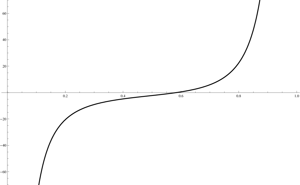
These results also show explicitly the terms that are responsible for the ambiguity in the Casimir force. A closer look at these terms demonstrates that they are proportional to the heat kernel coefficients a(d+1)/2−ia_{(d+1)/2-i} of the manifold 𝒩\mathscr{N} with 0≤i≤[(d+1)/2]0\leq i\leq[(d+1)/2]. It is clear that this ambiguity in the prediction of the force disappears if the manifold 𝒩\mathscr{N} is even-dimensional without boundary. However, even if a suitable manifold is chosen for which the Casimir force on the piston is well defined, the formulas (III) and (IV) do not allow to extract any information about its sign analytically, instead a numerical study is necessary; see Section VI.

In the next section we will study the asymptotic behavior of the Casimir force on the piston when both aa and bb are large, and when a→0a\to 0, i.e. the piston approaches the conical singularity.

V Asymptotic Behavior of the Casimir force for both aa and bb large and for a→0a\to 0

In this section we will study the asymptotic behavior of the Casimir force for Dirichlet and Neumann boundary conditions when both the parameters aa and bb are large, namely b/a→1b/a\to 1. For this analysis, we will employ the arguments outlined in [45] for the case of concentric spheres. Moreover, we will describe in detail only the Dirichlet case, since the Neumann case can be treated in exactly the same way. In the limit b/a→1b/a\to 1 the Casimir force for the conical piston will reproduce the one for parallel plates. From the expressions (III) and (IV) it is not difficult to realize that all the terms but ℱ𝒟\mathscr{F}_{\mathcal{D}} and ℱ𝒩\mathscr{F}_{\mathcal{N}} vanish proportionally to a−2a^{-2} as a→∞a\to\infty. Therefore, the asymptotic behavior for aa and bb large when Dirichlet or Neumann boundary conditions are imposed is given, respectively, by ℱ𝒟\mathscr{F}_{\mathcal{D}} and ℱ𝒩\mathscr{F}_{\mathcal{N}}. With the last remark in mind we can write that, when b/a→1b/a\to 1,

FCasDir(a,b)∼−12​π∑νd(ν)ν∫0∞dκ∂∂a[1−Kν​(ν​κ​b)​Iν​(ν​κ​a)Kν​(ν​κ​a)​Iν​(ν​κ​b)].F^{\textrm{Dir}}_{\textrm{Cas}}(a,b)\sim-\frac{1}{2\pi}\sum_{\nu}d(\nu)\nu\int_{0}^{\infty}d\kappa\frac{\partial}{\partial a}\left[1-\frac{K_{\nu}(\nu\kappa b)I_{\nu}(\nu\kappa a)}{K_{\nu}(\nu\kappa a)I_{\nu}(\nu\kappa b)}\right]\;. (92)

The derivative in the integrand, denoted by 𝒫⁡(κ,a,b)\mathcal{P}(\kappa,a,b), can be evaluated my making use of the properties of the derivative of the modified Bessel functions to get

𝒫⁡(κ,a,b)=−Kν​(ν​κ​b)a​Kν2​(ν​κ​a)​Iν​(ν​κ​b)​[1−Kν​(ν​κ​b)​Iν​(ν​κ​a)Kν​(ν​κ​a)​Iν​(ν​κ​b)]−1.\mathcal{P}(\kappa,a,b)=-\frac{K_{\nu}(\nu\kappa b)}{aK^{2}_{\nu}(\nu\kappa a)I_{\nu}(\nu\kappa b)}\left[1-\frac{K_{\nu}(\nu\kappa b)I_{\nu}(\nu\kappa a)}{K_{\nu}(\nu\kappa a)I_{\nu}(\nu\kappa b)}\right]^{-1}\;. (93)

By performing the following change of variables κ→κ/a\kappa\to\kappa/a, we obtain the expression

FCasDir​(a,b)∼12​π​a2​∑νd⁡(ν)​ν​∫0∞d​κ​𝒫​(ν​κa,1,ba).F^{\textrm{Dir}}_{\textrm{Cas}}(a,b)\sim\frac{1}{2\pi a^{2}}\sum_{\nu}d(\nu)\nu\int_{0}^{\infty}d\kappa\,\mathcal{P}\left(\frac{\nu\kappa}{a},1,\frac{b}{a}\right)\;. (94)

The b→ab\to a behavior of the Casimir force is already captured using the uniform asymptotic expansion of the modified Bessel functions to obtain [45]

𝒫⁡(ν​κa,1,ba)∼2​ν​1+κ2​∑n=1∞e−2​n​ν​[η⁡(b​κa)−η⁡(κ)]​∑i=0∞pi​(t,a,b,n)νi,\mathcal{P}\left(\frac{\nu\kappa}{a},1,\frac{b}{a}\right)\sim 2\nu\sqrt{1+\kappa^{2}}\sum_{n=1}^{\infty}e^{-2n\nu\left[\eta\left(\frac{b\kappa}{a}\right)-\eta(\kappa)\right]}\sum_{i=0}^{\infty}\frac{p_{i}(t,a,b,n)}{\nu^{i}}\;, (95)

where pip_{i} are polynomials in tt which vanish when b→ab\to a and such that p0=1p_{0}=1 [45]. By utilizing the inverse Mellin transform we can rewrite the sum of the exponentials in (95) in terms of a complex integral as follows

∑n=1∞e−2​n​ν​[η⁡(b​κa)−η⁡(κ)]=∑n=1∞12​π​i​∫c−i​∞c+i​∞d​α​Γ​(α)​(2​n​ν)−α​[η⁡(b​κa)−η⁡(κ)]−α,\sum_{n=1}^{\infty}e^{-2n\nu\left[\eta\left(\frac{b\kappa}{a}\right)-\eta(\kappa)\right]}=\sum_{n=1}^{\infty}\frac{1}{2\pi i}\int_{c-i\infty}^{c+i\infty}d\alpha\,\Gamma(\alpha)(2n\nu)^{-\alpha}\left[\eta\left(\frac{b\kappa}{a}\right)-\eta(\kappa)\right]^{-\alpha}\;, (96)

which is valid for ℜ⁡(ν)>0\Re(\nu)>0, and we assume that ℜ⁡(c)\Re(c) is large enough so that the sum over ν\nu and the integral in α\alpha can be safely interchanged.

By substituting the expressions (95) and (96) into the integral (94), and by recalling the definition of ζ𝒩\zeta_{\mathscr{N}} in (12) we obtain

FCasDir​(a,b)∼12​π2​i​a2​∑i=0∞∫c−i​∞c+i​∞d​α​Γ​(α)​(2)−α​ζR​(α)​ζ𝒩​(α+i2−1)\displaystyle F^{\textrm{Dir}}_{\textrm{Cas}}(a,b)\sim\frac{1}{2\pi^{2}i\,a^{2}}\sum_{i=0}^{\infty}\int_{c-i\infty}^{c+i\infty}d\alpha\,\Gamma(\alpha)(2)^{-\alpha}\zeta_{R}(\alpha)\zeta_{\mathscr{N}}\left(\frac{\alpha+i}{2}-1\right)
×∫0∞d​κ​1+κ2​[η⁡(b​κa)−η⁡(κ)]−α​pi​(t,a,b,n),\displaystyle\times\int_{0}^{\infty}d\kappa\sqrt{1+\kappa^{2}}\left[\eta\left(\frac{b\kappa}{a}\right)-\eta(\kappa)\right]^{-\alpha}p_{i}(t,a,b,n)\;, (97)

where the integral over κ\kappa is convergent for ℜ⁡(c)>2\Re(c)>2, since η⁡(b​κ/a)−η⁡(κ)→ln⁡(b/a)\eta\left(b\kappa/a\right)-\eta(\kappa)\to\ln(b/a) as κ→0\kappa\to 0 and η⁡(b​κ/a)−η⁡(κ)→(b/a−1)​κ\eta\left(b\kappa/a\right)-\eta(\kappa)\to(b/a-1)\kappa as κ→∞\kappa\to\infty [45].

It is convenient, at this point, to introduce the variable q=b/a−1q=b/a-1. In this new variable the limit we are interested in corresponds to q→0q\to 0. The leading behavior in qq of the integral (97) is given by the term with i=0i=0, since the other polynomials pip_{i}, with i≥1i\geq 1, vanish as q→0q\to 0, more explicitly

FCasDir​(q)∼12​π2​i​a2​∫c−i​∞c+i​∞d​α​Γ​(α)​(2)−α​ζR​(α)​ζ𝒩​(α2−1)​∫0∞d​κ​1+κ2​[η⁡((q+1)​κ)−η⁡(κ)]−α.F^{\textrm{Dir}}_{\textrm{Cas}}(q)\sim\frac{1}{2\pi^{2}i\,a^{2}}\int_{c-i\infty}^{c+i\infty}d\alpha\,\Gamma(\alpha)(2)^{-\alpha}\zeta_{R}(\alpha)\zeta_{\mathscr{N}}\left(\frac{\alpha}{2}-1\right)\int_{0}^{\infty}d\kappa\sqrt{1+\kappa^{2}}\left[\eta\left((q+1)\kappa\right)-\eta(\kappa)\right]^{-\alpha}\;. (98)

By closing the contour to the right, we encounter all poles of ζ𝒩\zeta_{\mathscr{N}} with ℜ⁡(α)>2\Re(\alpha)>2. The rightmost pole of ζ𝒩\zeta_{\mathscr{N}} results from α=d+2\alpha=d+2, the other poles further to the left will be irrelevant for what follows because the leading behavior of (98) as q→0q\to 0 is proportional to the residue of ζ𝒩​(α/2−1)\zeta_{\mathscr{N}}(\alpha/2-1) at α=d+2\alpha=d+2. This is seen by using [45]

η⁡((q+1)​κ)−η⁡(κ)=q​1+κ2+O⁡(q2).\eta\left((q+1)\kappa\right)-\eta(\kappa)=q\sqrt{1+\kappa^{2}}+O(q^{2})\;. (99)

The last remark, and the expansion (99), allow us to obtain the Casimir force for the conical piston endowed with Dirichlet boundary conditions when b/a→1b/a\to 1 as follows

FCasDir​(q)=Γ⁡(D+1)​ζR​(D+1)2D+1​π​Γ​(D2)​𝒜0𝒩qD+1+O⁡(q−D),F^{\textrm{Dir}}_{\textrm{Cas}}(q)=\frac{\Gamma(D+1)\zeta_{R}(D+1)}{2^{D+1}\sqrt{\pi}\,\Gamma\left(\frac{D}{2}\right)}\frac{\mathscr{A}^{\mathscr{N}}_{0}}{q^{D+1}}+O\left(q^{-D}\right)\;, (100)

where the higher orders in qq would involve the other heat kernel coefficients of 𝒩\mathscr{N}. The Neumann case is treated in exactly the same way and the resulting Casimir force when b/a→1b/a\to 1 reduces to (100).

Let us now turn our attention to the limiting behavior of the Casimir force when the piston approaches the conical singularity, namely, when a→0a\to 0. From the expressions (III) and (IV) it is not difficult to observe that all the terms, except ℱ𝒟\mathscr{F}_{\mathcal{D}} and ℱ𝒩\mathscr{F}_{\mathcal{N}}, are proportional to a−2a^{-2}. The proportionality coefficient and its sign will depend on the specific geometry of the piston 𝒩\mathscr{N}. It is therefore sufficient to study the asymptotics of ℱ𝒟\mathscr{F}_{\mathcal{D}} and ℱ𝒩\mathscr{F}_{\mathcal{N}} as a→0a\to 0. Once again, we will focus on the Dirichlet case since the Neumann case can be treated in exactly the same way.

From the expressions (38) and (93), by exploiting the change of variables κ→κ/ν\kappa\to\kappa/\nu, we can write

−12ℱ𝒟′(−12,a,b)=−12​π∑νd(ν)ν∫0∞dκ𝒫(κν,a,b).-\frac{1}{2}\mathscr{F}^{\prime}_{\mathcal{D}}\left(-\frac{1}{2},a,b\right)=-\frac{1}{2\pi}\sum_{\nu}d(\nu)\nu\int_{0}^{\infty}d\kappa\,\mathcal{P}\left(\frac{\kappa}{\nu},a,b\right)\;. (101)

Since we are interested in the small aa expansion, we utilize the series representation of the modified Bessel functions to obtain the following expression, to leading order in aa, of (93)

𝒫⁡(κν,a,b)=4Γ2​(ν)​a2​ν−1​Kν​(κ​b)Iν​(κ​b)​(κ2)2​ν+O⁡(κ2​ν+2).\mathcal{P}\left(\frac{\kappa}{\nu},a,b\right)=\frac{4}{\Gamma^{2}(\nu)}a^{2\nu-1}\frac{K_{\nu}(\kappa b)}{I_{\nu}(\kappa b)}\left(\frac{\kappa}{2}\right)^{2\nu}+O\left(\kappa^{2\nu+2}\right)\;. (102)

This expansion allows us to write

−12​ℱ𝒟′​(−12,a,b)=2π​∑νd⁡(ν)​a2​ν−1Γ2​(ν)​∫0∞d​κ​Kν​(κ​b)Iν​(κ​b)​(κ2)2​ν+O⁡(κ2​ν+2).-\frac{1}{2}\mathscr{F}^{\prime}_{\mathcal{D}}\left(-\frac{1}{2},a,b\right)=\frac{2}{\pi}\sum_{\nu}d(\nu)\frac{a^{2\nu-1}}{\Gamma^{2}(\nu)}\int_{0}^{\infty}d\kappa\frac{K_{\nu}(\kappa b)}{I_{\nu}(\kappa b)}\left(\frac{\kappa}{2}\right)^{2\nu}+O\left(\kappa^{2\nu+2}\right)\;. (103)

The integral in the last expression is convergent, since

Kν​(κ​b)Iν​(κ​b)​(κ2)2​ν∼12​Γ​(ν)​Γ​(ν+1)​b−2​ν,forκ→0,\frac{K_{\nu}(\kappa b)}{I_{\nu}(\kappa b)}\left(\frac{\kappa}{2}\right)^{2\nu}\sim\frac{1}{2}\Gamma(\nu)\Gamma(\nu+1)b^{-2\nu}\;,\quad\textrm{for}\quad\kappa\to 0\;, (104)

and

Kν​(κ​b)Iν​(κ​b)​(κ2)2​ν∼π​e−2​κ​(κ2)2​ν,forκ→∞.\frac{K_{\nu}(\kappa b)}{I_{\nu}(\kappa b)}\left(\frac{\kappa}{2}\right)^{2\nu}\sim\pi e^{-2\kappa}\left(\frac{\kappa}{2}\right)^{2\nu}\;,\quad\textrm{for}\quad\kappa\to\infty\;. (105)

We can therefore conclude that for ν>−1/2\nu>-1/2, which is within the assumptions of our work, the contribution ℱ𝒟′\mathscr{F}^{\prime}_{\mathcal{D}} is subleading as a→0a\to 0.

The previous arguments show that as a→0a\to 0 the Casimir force on the piston possesses a behavior of the type a−2a^{-2} with the proportionality coefficient depending on ζ𝒩\zeta_{\mathscr{N}} and, hence, on the geometry of the piston.

In the next section we will study a particular case in which the manifold 𝒩\mathscr{N} is a dd-dimensional sphere. This case is of special interest because the spectral zeta function of a dd-dimensional sphere can be explicitly evaluated in terms of a linear combination of Hurwitz ζ\zeta-functions [7, 15, 34].

VI A Specific Piston: The dd-dimensional Sphere

In this section we will study the case in which the base manifold is a dd-dimensional sphere. In this particular situation the eigenvalues of the Laplacian on 𝒩{\mathscr{N}} are known to be

ν=(l+d−12),\nu=\left(l+\frac{d-1}{2}\right)\;, (106)

with l≥0l\geq 0, and the eigenfunctions are hyperspherical harmonics with degeneracy

d⁡(l)=(2​l+d−1)​(l+d−2)!l!​(d−1)!.d(l)=(2l+d-1)\frac{(l+d-2)!}{l!(d-1)!}\;. (107)

The explicit knowledge of the eigenvalues ν\nu and their degeneracy allows us to write the ζ\zeta-function on 𝒩{\mathscr{N}} as follows

ζ𝒩​(s)=∑l=0∞(2​l+d−1)​(l+d−2)!l!​(d−1)!​(l+d−12)−2​s.\zeta_{{\mathscr{N}}}(s)=\sum_{l=0}^{\infty}(2l+d-1)\frac{(l+d-2)!}{l!(d-1)!}\left(l+\frac{d-1}{2}\right)^{-2s}\;. (108)

The previous expression can be conveniently rewritten in terms of a linear combination of Hurwitz ζ\zeta-functions, namely [7, 8]

ζ𝒩​(s)=2​∑α=0d−1eα​ζH​(2​s−α−1,d−12),\zeta_{{\mathscr{N}}}(s)=2\sum_{\alpha=0}^{d-1}e_{\alpha}\zeta_{H}\left(2s-\alpha-1,\frac{d-1}{2}\right)\;, (109)

where the coefficients eαe_{\alpha} are defined through the relation

(l+d−2)!l!​(d−1)!=∑α=0d−1eα​(l+d−12)α.\frac{(l+d-2)!}{l!(d-1)!}=\sum_{\alpha=0}^{d-1}e_{\alpha}\left(l+\frac{d-1}{2}\right)^{\alpha}\;. (110)

As one can easily see, from the general results (III) and (IV), we need to compute either the value or the residue or the finite part of the spectral ζ\zeta-function on the manifold 𝒩\mathscr{N} at specific points. For s=−m/2s=-m/2, with m≥−1m\geq-1, by utilizing the equation (109), we obtain the result [2, 3, 15, 19]

ζ𝒩(−m2)=−2∑α=0d−1eαm+α+2Bm+α+2(d−12),\zeta_{\mathscr{N}}\left(-\frac{m}{2}\right)=-2\sum_{\alpha=0}^{d-1}\frac{e_{\alpha}}{m+\alpha+2}B_{m+\alpha+2}\left(\frac{d-1}{2}\right)\;, (111)

where we have used the relation, valid for n≥0n\geq 0 [31],

ζH​(−n,q)=−Bn+1​(q)n+1,\zeta_{H}(-n,q)=-\frac{B_{n+1}(q)}{n+1}\;, (112)

with Bn​(q)B_{n}(q) being the Bernoulli polynomials. It is clear from the relation (111) that the residue of ζ𝒩​(s)\zeta_{\mathscr{N}}(s) at s=−1/2s=-1/2 and s=1/2s=1/2 vanish.

The remaining values of ss that we need to analyze are the ones of the form s=m/2s=m/2 with m≥0m\geq 0. It is well known that the Hurwitz ζ\zeta-function, ζH​(s,q)\zeta_{H}(s,q), has a simple pole at s=1s=1. The explicit form of its Laurent expansion depends on whether qq is an integer or a half-integer. In fact, for q=n+1/2q=n+1/2, with n≥0n\geq 0, we have

ζH​(1+ε​x,n+12)=1ε​x+γ+2​ln⁡2−2​∑k=1n12​k−1+O⁡(x),\zeta_{H}\left(1+\varepsilon x,n+\frac{1}{2}\right)=\frac{1}{\varepsilon x}+\gamma+2\ln 2-2\sum_{k=1}^{n}\frac{1}{2k-1}+O(x)\;, (113)

while for q=nq=n and n≥0n\geq 0 we obtain

ζH​(1+ε​x,n)=1ε​x+γ−∑k=1n−11k+O⁡(x).\zeta_{H}\left(1+\varepsilon x,n\right)=\frac{1}{\varepsilon x}+\gamma-\sum_{k=1}^{n-1}\frac{1}{k}+O(x)\;. (114)

By utilizing the above results and the relation (109) we obtain the following expression for the residue of ζ𝒩​(s)\zeta_{\mathscr{N}}(s) at s=m/2s=m/2 with d≥m≥2d\geq m\geq 2,

Res​ζ𝒩​(m2)=em−2,\textrm{Res}\,\zeta_{\mathscr{N}}\left(\frac{m}{2}\right)=e_{m-2}\;, (115)

the contribution to the residue coming from the index α=m−2\alpha=m-2 of the summation in (109). According to (113) and (114), for the finite part at s=m/2s=m/2 we have to distinguish between two cases. If the dimension dd of the manifold 𝒩\mathscr{N} is even, then

FP​ζ𝒩​(m2)=2​∑α=0α≠m−2d−1eα​ζH​(m−α−1,d−12)+2​em−2​(γ+2​ln⁡2−2​∑k=1d2−112​k−1),\textrm{FP}\,\zeta_{\mathscr{N}}\left(\frac{m}{2}\right)=2\sum_{{\alpha=0\atop\alpha\neq m-2}}^{d-1}e_{\alpha}\zeta_{H}\left(m-\alpha-1,\frac{d-1}{2}\right)+2e_{m-2}\left(\gamma+2\ln 2-2\sum_{k=1}^{\frac{d}{2}-1}\frac{1}{2k-1}\right)\;, (116)

while if dd is odd, we have

FP​ζ𝒩​(m2)=2​∑α=0α≠m−2d−1eα​ζH​(m−α−1,d−12)+2​em−2​(γ−∑k=1d−3212​k−1).\textrm{FP}\,\zeta_{\mathscr{N}}\left(\frac{m}{2}\right)=2\sum_{{\alpha=0\atop\alpha\neq m-2}}^{d-1}e_{\alpha}\zeta_{H}\left(m-\alpha-1,\frac{d-1}{2}\right)+2e_{m-2}\left(\gamma-\sum_{k=1}^{\frac{d-3}{2}}\frac{1}{2k-1}\right)\;. (117)

The results that we have obtained in this section so far are well suited for the analysis of conical pistons with Dirichlet boundary conditions. However, the case of Neumann boundary conditions needs a special treatment when the manifold 𝒩\mathscr{N} is a dd-dimensional sphere. In fact, from the integral representation (63) of the spectral ζ\zeta-function in region II, one can notice that the case l=0l=0, namely ν=(d−1)/2\nu=(d-1)/2, needs particular care because the behavior of (β​Id−12​(a​k)+a​k​Id−12′​(a​k))\left(\beta I_{\frac{d-1}{2}}(ak)+akI^{\prime}_{\frac{d-1}{2}}(ak)\right) as k→0k\to 0 is different. This corresponds, according to (106), to the lowest angular eigenvalue ν\nu. In this case, in fact, we have the following small kk expansion

(β​Id−12​(a​k)+a​k​Id−12′​(a​k))=(a​k)d+322d+12​Γ​(d+32)+O⁡(kd+72).\left(\beta I_{\frac{d-1}{2}}(ak)+akI^{\prime}_{\frac{d-1}{2}}(ak)\right)=\frac{(ak)^{\frac{d+3}{2}}}{2^{\frac{d+1}{2}}\Gamma\left(\frac{d+3}{2}\right)}+O\left(k^{\frac{d+7}{2}}\right)\;. (118)

The above expansion suggests that a more suitable integral representation for the contribution of the mode ν=(d−1)/2\nu=(d-1)/2 is the following

ζI𝒩,l=0​(s,a)=a2​s​(d−12)​sin⁡(π​s)π​∫0∞d​k​k−2​s​∂∂k​ln⁡[k−d+32​(β​Id−12​(k)+k​Id−12′​(k))],\zeta^{\mathcal{N},\,l=0}_{I}(s,a)=a^{2s}\left(\frac{d-1}{2}\right)\frac{\sin(\pi s)}{\pi}\int_{0}^{\infty}dk\,k^{-2s}\frac{\partial}{\partial k}\ln\left[k^{-\frac{d+3}{2}}\left(\beta I_{\frac{d-1}{2}}(k)+kI^{\prime}_{\frac{d-1}{2}}(k)\right)\right]\;, (119)

which is valid in the strip 1/2<ℜ⁡(s)<11/2<\Re(s)<1. In order to analytically continue the above expression in the neighborhood of s=−1/2s=-1/2, we utilize the following k→∞k\to\infty asymptotic expansion

ln⁡[k−d+32​(β​Id−12​(k)+k​Id−12′​(k))]∼ln⁡[k−d2−12​π​ek]+∑n=1∞ℬn​(d−12)kn,\ln\left[k^{-\frac{d+3}{2}}\left(\beta I_{\frac{d-1}{2}}(k)+kI^{\prime}_{\frac{d-1}{2}}(k)\right)\right]\sim\ln\left[\frac{k^{-\frac{d}{2}-1}}{\sqrt{2\pi}}\,e^{k}\right]+\sum_{n=1}^{\infty}\frac{\mathcal{B}_{n}\left(\frac{d-1}{2}\right)}{k^{n}}\;, (120)

where the polynomials are defined according to the relation

[1+∑n=1∞(−1)n​rn​(d−12)kn+1−d2​k​(1+∑n=1∞(−1)n​pn​(d−12)kn)]∼∑n=1∞ℬn​(d−12)kn.\left[1+\sum_{n=1}^{\infty}(-1)^{n}\frac{r_{n}\left(\frac{d-1}{2}\right)}{k^{n}}+\frac{1-d}{2k}\left(1+\sum_{n=1}^{\infty}(-1)^{n}\frac{p_{n}\left(\frac{d-1}{2}\right)}{k^{n}}\right)\right]\sim\sum_{n=1}^{\infty}\frac{\mathcal{B}_{n}\left(\frac{d-1}{2}\right)}{k^{n}}\;. (121)

The expressions (120) and (121) can be obtained by exploiting the asymptotic expansions for z→∞z\to\infty [39],

Iν​(z)∼ez2​π​z​[1+∑n=1∞rn​(ν)zn]andIν′​(z)∼ez2​π​z​[1+∑n=1∞pn​(ν)zn],I_{\nu}(z)\sim\frac{e^{z}}{\sqrt{2\pi z}}\left[1+\sum_{n=1}^{\infty}\frac{r_{n}(\nu)}{z^{n}}\right]\;\quad\textrm{and}\quad I^{\prime}_{\nu}(z)\sim\frac{e^{z}}{\sqrt{2\pi z}}\left[1+\sum_{n=1}^{\infty}\frac{p_{n}(\nu)}{z^{n}}\right]\;, (122)

where the functions rn​(x)r_{n}(x) and pn​(x)p_{n}(x) are obtained from the relations

r0​(x)=1,r1​(x)=4​x2+38,rn​(x)=4​x2+4​n2−1n!​8n​∏i=2n[4​x2−(2​i−3)2],r_{0}(x)=1\;,\quad r_{1}(x)=\frac{4x^{2}+3}{8}\;,\quad r_{n}(x)=\frac{4x^{2}+4n^{2}-1}{n!8^{n}}\prod_{i=2}^{n}\left[4x^{2}-(2i-3)^{2}\right]\;, (123)

and

p0​(x)=1,pn​(x)=1n!​8n​∏i=1n[4​x2−(2​i−1)2].p_{0}(x)=1\;,\quad p_{n}(x)=\frac{1}{n!8^{n}}\prod_{i=1}^{n}\left[4x^{2}-(2i-1)^{2}\right]\;. (124)

At this point it will be sufficient, for our purposes, to add and subtract the leading term of the expansion to obtain the result which is valid for −1<ℜ⁡(s)<1/2-1<\Re(s)<1/2,

ζI𝒩,l=0​(s,a)\displaystyle\zeta^{\mathcal{N},\,l=0}_{I}(s,a) =\displaystyle= WIl=0(s,a)−a2​ssin⁡(π​s)π(d−12){(d2+1)12​s−12​s−1\displaystyle W^{l=0}_{I}(s,a)-a^{2s}\frac{\sin(\pi s)}{\pi}\left(\frac{d-1}{2}\right)\Bigg\{\left(\frac{d}{2}+1\right)\frac{1}{2s}-\frac{1}{2s-1} (125)
−\displaystyle- 12​s+1(38+d−12+(d−1)28)},\displaystyle\frac{1}{2s+1}\left(\frac{3}{8}+\frac{d-1}{2}+\frac{(d-1)^{2}}{8}\right)\Bigg\}\;,

where

WIl=0​(s,a)\displaystyle W^{l=0}_{I}(s,a) =\displaystyle= a2​s(d−12)sin⁡(π​s)π∫0∞dkk−2​s∂∂k{ln[k−d+32(βId−12(k)+kId−12′(k))]\displaystyle a^{2s}\left(\frac{d-1}{2}\right)\frac{\sin(\pi s)}{\pi}\int_{0}^{\infty}dk\,k^{-2s}\frac{\partial}{\partial k}\Bigg\{\ln\left[k^{-\frac{d+3}{2}}\left(\beta I_{\frac{d-1}{2}}(k)+kI^{\prime}_{\frac{d-1}{2}}(k)\right)\right] (126)
−\displaystyle- H(k−1)[ln(k−d2−12​πek)−1k(38+d−12+(d−1)28)]},\displaystyle H(k-1)\Bigg[\ln\left(\frac{k^{-\frac{d}{2}-1}}{\sqrt{2\pi}}\,e^{k}\right)-\frac{1}{k}\left(\frac{3}{8}+\frac{d-1}{2}+\frac{(d-1)^{2}}{8}\right)\Bigg]\Bigg\}\;,

with the step function H⁡(k)H(k). In region I​III a similar argument for the lowest angular eigenvalue is necessary. In fact by utilizing the small κ\kappa expansion of the modified Bessel functions, it is not very difficult to show that Ξd−12​(a,κ)\Xi_{\frac{d-1}{2}}(a,\kappa) in (65) behaves differently as κ→0\kappa\to 0. More specifically, one obtains

Ξd−12​(a,κ)=2​a2d+3​[(ab)−d+32−(ab)d−12]​(κ2)2+O⁡(κ416).\Xi_{\frac{d-1}{2}}(a,\kappa)=\frac{2a^{2}}{d+3}\left[\left(\frac{a}{b}\right)^{-\frac{d+3}{2}}-\left(\frac{a}{b}\right)^{\frac{d-1}{2}}\right]\left(\frac{\kappa}{2}\right)^{2}+O\left(\frac{\kappa^{4}}{16}\right)\;. (127)

A suitable representation for the spectral ζ\zeta-function in region I​III corresponding to the lowest eigenvalue is therefore

ζI​I𝒩,l=0​(s,a)\displaystyle\zeta^{\mathcal{N},\,l=0}_{II}(s,a) =\displaystyle= a2​s​(d−12)​sin⁡(π​s)π​∫0∞d​κ​κ−2​s​∂∂κ​ln⁡[κd−12​(−β​Kd−12​(κ)−κ​Kd−12′​(κ))]\displaystyle a^{2s}\left(\frac{d-1}{2}\right)\frac{\sin(\pi s)}{\pi}\int_{0}^{\infty}d\kappa\,\kappa^{-2s}\frac{\partial}{\partial\kappa}\ln\left[\kappa^{\frac{d-1}{2}}(-\beta K_{\frac{d-1}{2}}(\kappa)-\kappa K^{\prime}_{\frac{d-1}{2}}(\kappa))\right] (128)
+\displaystyle+ b2​s​(d−12)​sin⁡(π​s)π​∫0∞d​κ​κ−2​s​∂∂κ​ln⁡[κ−d+32​(β​Id−12​(κ)+κ​Id−12′​(κ))]\displaystyle b^{2s}\left(\frac{d-1}{2}\right)\frac{\sin(\pi s)}{\pi}\int_{0}^{\infty}d\kappa\,\kappa^{-2s}\frac{\partial}{\partial\kappa}\ln\left[\kappa^{-\frac{d+3}{2}}(\beta I_{\frac{d-1}{2}}(\kappa)+\kappa I^{\prime}_{\frac{d-1}{2}}(\kappa))\right]
+\displaystyle+ (d−12)​sin⁡(π​s)π​∫0∞d​κ​κ−2​s​∂∂κ​ln⁡Δd−12​(κ,a,b).\displaystyle\left(\frac{d-1}{2}\right)\frac{\sin(\pi s)}{\pi}\int_{0}^{\infty}d\kappa\,\kappa^{-2s}\frac{\partial}{\partial\kappa}\ln\Delta_{\frac{d-1}{2}}(\kappa,a,b)\;.

After analytic continuation of (128), we obtain the following result which is well defined in the region −1<ℜ⁡(s)<1/2-1<\Re(s)<1/2

ζI​I𝒩,l=0​(s,a,b)\displaystyle\zeta^{\mathcal{N},\,l=0}_{II}(s,a,b) =\displaystyle= WI​Il=0(s,a,b)+ℱ𝒩l=0(s,a,b)−sin⁡(π​s)π(d−12){12​s[b2​s−d2(a2​s−b2​s)]+a2​s−b2​s2​s−1\displaystyle W^{l=0}_{II}(s,a,b)+\mathscr{F}_{\mathcal{N}}^{l=0}(s,a,b)-\frac{\sin(\pi s)}{\pi}\left(\frac{d-1}{2}\right)\Bigg\{\frac{1}{2s}\left[b^{2s}-\frac{d}{2}\left(a^{2s}-b^{2s}\right)\right]+\frac{a^{2s}-b^{2s}}{2s-1} (129)
+\displaystyle+ 12​s+1(38+d−12+(d−1)28)(a2​s−b2​s)},\displaystyle\frac{1}{2s+1}\left(\frac{3}{8}+\frac{d-1}{2}+\frac{(d-1)^{2}}{8}\right)\left(a^{2s}-b^{2s}\right)\Bigg\}\;,

where WI​Il=0​(s,a,b)W^{l=0}_{II}(s,a,b) has the form

WI​Il=0​(s,a,b)\displaystyle W^{l=0}_{II}(s,a,b) =\displaystyle= (d−12)sin⁡(π​s)π∫0∞dκκ−2​s∂∂κ{a2​sln[κd−12(−βKd−12(κ)−κKd−12′(κ))]\displaystyle\left(\frac{d-1}{2}\right)\frac{\sin(\pi s)}{\pi}\int_{0}^{\infty}d\kappa\,\kappa^{-2s}\frac{\partial}{\partial\kappa}\Bigg\{a^{2s}\ln\left[\kappa^{\frac{d-1}{2}}\left(-\beta K_{\frac{d-1}{2}}(\kappa)-\kappa K^{\prime}_{\frac{d-1}{2}}(\kappa)\right)\right] (130)
+\displaystyle+ b2​sln[κ−d+32(βId−12(κ)+κId−12′(κ))]−H(κ−1)[a2​sln(π2κd2e−κ)+b2​sln(κ−d2−12​πeκ)\displaystyle b^{2s}\ln\left[\kappa^{-\frac{d+3}{2}}\left(\beta I_{\frac{d-1}{2}}(\kappa)+\kappa I^{\prime}_{\frac{d-1}{2}}(\kappa)\right)\right]-H(\kappa-1)\Bigg[a^{2s}\ln\left(\sqrt{\frac{\pi}{2}}\,\kappa^{\frac{d}{2}}e^{-\kappa}\right)+b^{2s}\ln\left(\frac{\kappa^{-\frac{d}{2}-1}}{\sqrt{2\pi}}\,e^{\kappa}\right)
+\displaystyle+ 1κ(38+d−12+(d−1)28)(a2​s−b2​s)]}.\displaystyle\frac{1}{\kappa}\left(\frac{3}{8}+\frac{d-1}{2}+\frac{(d-1)^{2}}{8}\right)\left(a^{2s}-b^{2s}\right)\Bigg]\Bigg\}\;.

Let us mention that ℱ𝒩l=0​(s,a,b)\mathscr{F}_{\mathcal{N}}^{l=0}(s,a,b) coincides with (77) once we set ν=(d−1)/2\nu=(d-1)/2.

From the above results, it is not difficult to obtain the residue and finite part for ζℳ𝒩,l=0\zeta_{\mathscr{M}}^{\mathcal{N},\,l=0} at s=−1/2s=-1/2 corresponding to the lowest angular eigenvalue. In more detail, we have

FP​ζℳ𝒩,l=0​(−12,a,b)=WIl=0​(−12,a)+WI​Il=0​(−12,a,b)+ℱ𝒩l=0​(−12,a,b)−d−12​π​(1a+d+12​b),\textrm{FP}\,\zeta_{\mathscr{M}}^{\mathcal{N},\,l=0}\left(-\frac{1}{2},a,b\right)=W^{l=0}_{I}\left(-\frac{1}{2},a\right)+W^{l=0}_{II}\left(-\frac{1}{2},a,b\right)+\mathscr{F}_{\mathcal{N}}^{l=0}\left(-\frac{1}{2},a,b\right)-\frac{d-1}{2\pi}\left(\frac{1}{a}+\frac{d+1}{2b}\right)\;, (131)

and

Res​ζℳ𝒩,l=0​(−12,a)=−d−14​π​b​(38+d−12+(d−1)28).\textrm{Res}\,\zeta_{\mathscr{M}}^{\mathcal{N},\,l=0}\left(-\frac{1}{2},a\right)=-\frac{d-1}{4\pi b}\left(\frac{3}{8}+\frac{d-1}{2}+\frac{(d-1)^{2}}{8}\right)\;. (132)

Therefore, the contribution of ν=(d−1)/2\nu=(d-1)/2 to the Casimir force on the piston when Neumann boundary conditions are imposed is, according to (16),

FCasNeu,l=0​(a)=−12​WI′l=0​(−12,a)−12​WI​I′l=0​(−12,a)−12​ℱ𝒩′l=0​(−12,a,b)−d−14​π​a2.F_{\textrm{Cas}}^{\textrm{Neu},\,l=0}(a)=-\frac{1}{2}W^{\prime\,l=0}_{I}\left(-\frac{1}{2},a\right)-\frac{1}{2}W^{\prime\,l=0}_{II}\left(-\frac{1}{2},a\right)-\frac{1}{2}\mathscr{F}_{\mathcal{N}}^{\prime\,l=0}\left(-\frac{1}{2},a,b\right)-\frac{d-1}{4\pi a^{2}}\;. (133)

Obviously, the total Casimir force on the piston for Neumann boundary conditions is the sum of (133) and (IV) where in the latter the lowest angular eigenvalue is omitted. In the next subsections we present explicit results for specific dimensions dd. We would like to point out that in the formulas that will follow it is understood that the functions ZZ, WW and ℱ\mathscr{F} are evaluated for the specific dimension under consideration.

VI.1 Specific Dimensions for Dirichlet Boundary Conditions

In the following special cases, we will set, for simplicity, b=1b=1. When the piston 𝒩\mathscr{N} is a sphere of dimension d=2d=2, and, therefore, the dimension of ℳ\mathscr{M} is D=3D=3, we obtain

FCasDir​(a)=−12​ZI′​(−12,a)−12​ZI​I′​(−12,a)−12​ℱD′​(−12,a).F_{\textrm{Cas}}^{\textrm{Dir}}(a)=-\frac{1}{2}Z^{\prime}_{I}\left(-\frac{1}{2},a\right)-\frac{1}{2}Z^{\prime}_{II}\left(-\frac{1}{2},a\right)-\frac{1}{2}\mathscr{F}^{\prime}_{D}\left(-\frac{1}{2},a\right)\;. (134)

For d=3d=3, or D=4D=4, we have the result

FCasDir​(a,α)\displaystyle F_{\textrm{Cas}}^{\textrm{Dir}}(a,\alpha) =\displaystyle= −12​ZI′​(−12,a)−12​ZI​I′​(−12,a)−12​ℱD′​(−12,a)+1a2​(2803983040+3565536​γ+35131072​ln⁡a2)\displaystyle-\frac{1}{2}Z^{\prime}_{I}\left(-\frac{1}{2},a\right)-\frac{1}{2}Z^{\prime}_{II}\left(-\frac{1}{2},a\right)-\frac{1}{2}\mathscr{F}^{\prime}_{D}\left(-\frac{1}{2},a\right)+\frac{1}{a^{2}}\Bigg(\frac{2803}{983040}+\frac{35}{65536}\gamma+\frac{35}{131072}\ln a^{2}\Bigg) (135)
+\displaystyle+ 35131072​a2​(1α+ln⁡μ2).\displaystyle\frac{35}{131072a^{2}}\left(\frac{1}{\alpha}+\ln\mu^{2}\right)\;.

For d=4d=4, or D=5D=5, we obtain

FCasDir​(a)\displaystyle F_{\textrm{Cas}}^{\textrm{Dir}}(a) =\displaystyle= −12​ZI′​(−12,a)−12​ZI​I′​(−12,a)−12​ℱD′​(−12,a)−35​π21572864​a2.\displaystyle-\frac{1}{2}Z^{\prime}_{I}\left(-\frac{1}{2},a\right)-\frac{1}{2}Z^{\prime}_{II}\left(-\frac{1}{2},a\right)-\frac{1}{2}\mathscr{F}^{\prime}_{D}\left(-\frac{1}{2},a\right)-\frac{35\pi^{2}}{1572864a^{2}}\;. (136)

And, finally, for d=5d=5, or D=6D=6, we get

FCasDir​(a,α)\displaystyle F_{\textrm{Cas}}^{\textrm{Dir}}(a,\alpha) =\displaystyle= −12​ZI′​(−12,a)−12​ZI​I′​(−12,a)−12​ℱD′​(−12,a)+1a2​(20377113246208−728525165824​γCLOSE\displaystyle-\frac{1}{2}Z^{\prime}_{I}\left(-\frac{1}{2},a\right)-\frac{1}{2}Z^{\prime}_{II}\left(-\frac{1}{2},a\right)-\frac{1}{2}\mathscr{F}^{\prime}_{D}\left(-\frac{1}{2},a\right)+\frac{1}{a^{2}}\Bigg(\frac{20377}{113246208}-\frac{7285}{25165824}\gamma (137)
−\displaystyle- OPEN168550331648​ln⁡a2+56525165824​ζR​(3))−168550331648​a2​(1α+ln⁡μ2).\displaystyle\frac{1685}{50331648}\ln a^{2}+\frac{565}{25165824}\zeta_{R}(3)\Bigg)-\frac{1685}{50331648a^{2}}\left(\frac{1}{\alpha}+\ln\mu^{2}\right)\;.

As mentioned previously we can see, from the above results that the Casimir force on the piston is not a well defined quantity when the piston 𝒩\mathscr{N} is odd dimensional. The Casimir force on the piston for d=2d=2 and d=4d=4, is shown in Figure 1. We can see that, for d=2d=2, the piston is repelled from the conical singularity and attracted to the base manifold positioned at b=1b=1. For d=4d=4, instead, a point of unstable equilibrium is present. If the piston is to the left of this point, it is attracted to the conical singularity. If it is to its right, then the piston is attracted to the base manifold.


Refer to caption
(a)  d=2d=2 (D=3D=3)
Refer to caption
(b)  d=4d=4 (D=5D=5)
Figure 1: Plots of the Casimir force, FCasDir​(a)F_{\textrm{Cas}}^{\textrm{Dir}}(a), on the piston 𝒩\mathscr{N} for Dirichlet boundary conditions as a function of the position aa.

VI.2 Specific Dimensions for Neumann Boundary Conditions

For Neumann boundary conditions, we need to consider the results obtained in (IV), with the lowest angular eigenvalue omitted, and the one obtained in (133). It is useful to stress that the spectral ζ\zeta-function ζ¯𝒩​(s)\bar{\zeta}_{\mathscr{N}}(s) with the lowest angular eigenvalue omitted is related to the ordinary ζ𝒩​(s)\zeta_{\mathscr{N}}(s) through the relation

ζ¯𝒩​(s)=ζ𝒩​(s)−(d−12)−2​s.\bar{\zeta}_{\mathscr{N}}(s)=\zeta_{\mathscr{N}}(s)-\left(\frac{d-1}{2}\right)^{-2s}\;. (138)

This expression is utilized in the results that will follow in order to obtain the Neumann Casimir force.

For d=2d=2, thus D=3D=3, we have the following expression for the force

FCasNeu​(a)\displaystyle F_{\textrm{Cas}}^{\textrm{Neu}}(a) =\displaystyle= −12​WI′l=0​(−12,a)−12​WI​I′l=0​(−12,a)−12​ℱ𝒩′l=0​(−12,a)−12​WI′​(−12,a)\displaystyle-\frac{1}{2}W^{\prime\,l=0}_{I}\left(-\frac{1}{2},a\right)-\frac{1}{2}W^{\prime\,l=0}_{II}\left(-\frac{1}{2},a\right)-\frac{1}{2}\mathscr{F}_{\mathcal{N}}^{\prime\,l=0}\left(-\frac{1}{2},a\right)-\frac{1}{2}W^{\prime}_{I}\left(-\frac{1}{2},a\right) (139)
−\displaystyle- 12​WI​I′​(−12,a)−12​ℱ𝒩′​(−12,a)−1a2​(14​π+27512).\displaystyle\frac{1}{2}W^{\prime}_{II}\left(-\frac{1}{2},a\right)-\frac{1}{2}\mathscr{F}^{\prime}_{\mathcal{N}}\left(-\frac{1}{2},a\right)-\frac{1}{a^{2}}\left(\frac{1}{4\pi}+\frac{27}{512}\right)\;.

For d=3d=3, thus D=4D=4, we have the result

FCasNeu​(a,α)\displaystyle F_{\textrm{Cas}}^{\textrm{Neu}}(a,\alpha) =\displaystyle= −12​WI′l=0​(−12,a)−12​WI​I′l=0​(−12,a)−12​ℱ𝒩′l=0​(−12,a)−12​WI′​(−12,a)\displaystyle-\frac{1}{2}W^{\prime\,l=0}_{I}\left(-\frac{1}{2},a\right)-\frac{1}{2}W^{\prime\,l=0}_{II}\left(-\frac{1}{2},a\right)-\frac{1}{2}\mathscr{F}_{\mathcal{N}}^{\prime\,l=0}\left(-\frac{1}{2},a\right)-\frac{1}{2}W^{\prime}_{I}\left(-\frac{1}{2},a\right) (140)
−\displaystyle- 12​WI​I′​(−12,a)−12​ℱ𝒩′​(−12,a)+1a2​(−12​π+1286932768−586165536​γ−5861131072​ln⁡a2)\displaystyle\frac{1}{2}W^{\prime}_{II}\left(-\frac{1}{2},a\right)-\frac{1}{2}\mathscr{F}^{\prime}_{\mathcal{N}}\left(-\frac{1}{2},a\right)+\frac{1}{a^{2}}\left(-\frac{1}{2\pi}+\frac{12869}{32768}-\frac{5861}{65536}\gamma-\frac{5861}{131072}\ln a^{2}\right)
−\displaystyle- 5861131072​a2​(1α+ln⁡μ2).\displaystyle\frac{5861}{131072a^{2}}\left(\frac{1}{\alpha}+\ln\mu^{2}\right)\;.

For d=4d=4, thus D=5D=5, we obtain

FCasNeu​(a)\displaystyle F_{\textrm{Cas}}^{\textrm{Neu}}(a) =\displaystyle= −12​WI′l=0​(−12,a)−12​WI​I′l=0​(−12,a)−12​ℱ𝒩′l=0​(−12,a)−12​WI′​(−12,a)\displaystyle-\frac{1}{2}W^{\prime\,l=0}_{I}\left(-\frac{1}{2},a\right)-\frac{1}{2}W^{\prime\,l=0}_{II}\left(-\frac{1}{2},a\right)-\frac{1}{2}\mathscr{F}_{\mathcal{N}}^{\prime\,l=0}\left(-\frac{1}{2},a\right)-\frac{1}{2}W^{\prime}_{I}\left(-\frac{1}{2},a\right) (141)
−\displaystyle- 12​WI​I′​(−12,a)−12​ℱ𝒩′​(−12,a)+1a2​(−34​π+57781221184+272531572864​π2).\displaystyle\frac{1}{2}W^{\prime}_{II}\left(-\frac{1}{2},a\right)-\frac{1}{2}\mathscr{F}^{\prime}_{\mathcal{N}}\left(-\frac{1}{2},a\right)+\frac{1}{a^{2}}\Bigg(-\frac{3}{4\pi}+\frac{57781}{221184}+\frac{27253}{1572864}\pi^{2}\Bigg)\;.

And, finally, for d=5d=5, thus D=6D=6, we get

FCasNeu​(a,α)\displaystyle F_{\textrm{Cas}}^{\textrm{Neu}}(a,\alpha) =\displaystyle= −12​WI′l=0​(−12,a)−12​WI​I′l=0​(−12,a)−12​ℱ𝒩′l=0​(−12,a)−12​WI′​(−12,a)\displaystyle-\frac{1}{2}W^{\prime\,l=0}_{I}\left(-\frac{1}{2},a\right)-\frac{1}{2}W^{\prime\,l=0}_{II}\left(-\frac{1}{2},a\right)-\frac{1}{2}\mathscr{F}_{\mathcal{N}}^{\prime\,l=0}\left(-\frac{1}{2},a\right)-\frac{1}{2}W^{\prime}_{I}\left(-\frac{1}{2},a\right) (142)
−\displaystyle- 12​WI​I′​(−12,a)−12​ℱ𝒩′​(−12,a)+1a2​(−1π+53466379829126835752960−172378316777216​γCLOSE\displaystyle\frac{1}{2}W^{\prime}_{II}\left(-\frac{1}{2},a\right)-\frac{1}{2}\mathscr{F}^{\prime}_{\mathcal{N}}\left(-\frac{1}{2},a\right)+\frac{1}{a^{2}}\Bigg(-\frac{1}{\pi}+\frac{53466379829}{126835752960}-\frac{1723783}{16777216}\gamma
−\displaystyle- OPEN172378333554432​ln⁡a2+1038178150331648​ζR​(3))−172378333554432​a2​(1α+ln⁡μ2).\displaystyle\frac{1723783}{33554432}\ln a^{2}+\frac{10381781}{50331648}\zeta_{R}(3)\Bigg)-\frac{1723783}{33554432a^{2}}\left(\frac{1}{\alpha}+\ln\mu^{2}\right)\;.

Once again, we would like to point out that also for Neumann boundary conditions the Casimir force on 𝒩\mathscr{N} is not well defined when dd is odd. The Casimir force on the piston for d=2d=2 and d=4d=4, is shown in Figure 2. We can notice that in both cases, namely d=2d=2 and d=4d=4, there exists a point of unstable equilibrium. If the piston is to the left of this point it is attracted to the conical singularity, while, if it is on its right, it is attracted to the base manifold.


Refer to caption
(a)  d=2d=2, and D=3D=3
Refer to caption
(b)  d=4d=4, and D=5D=5
Figure 2: Plots of the Casimir force, FCasNeu​(a)F_{\textrm{Cas}}^{\textrm{Neu}}(a), on the piston 𝒩\mathscr{N} for Neuman boundary conditions as function of the position aa.

VII Concluding Remarks

In this paper we have analyzed the Casimir effect for massless scalar fields in the setting of the bounded generalized cone in the cases in which the field is endowed with either Dirichlet or Neuman boundary conditions. The piston geometry has been obtained by dividing the generalized cone ℳ\mathscr{M} into two regions separated by its cross section positioned at aa with a∈(0,1)a\in(0,1). The cross section itself represents the piston, and the structure so obtained has been denoted conical piston. By utilizing ζ\zeta-function regularization methods, we have obtained very general results for the Casimir energy and, hence, for the corresponding Casimir force. The expressions obtained for the Casimir force are valid for any piston 𝒩\mathscr{N} and any dimension DD and are written in terms of the spectral ζ\zeta-function ζ𝒩\zeta_{\mathscr{N}}. In order to obtain more specific results, we have considered in detail the case when the manifold 𝒩\mathscr{N} is a dd-dimensional sphere. Explicit numerical results for this case have also been obtained for d=2d=2 and d=4d=4.

We would like to stress that this work provides a study of a piston geometry that is more general than the ones considered in the literature where the two chambers have fundamentally the same type of geometry. The two separate regions of the conical piston, instead, have different geometries since one of them contains a singularity while the other does not. This is the feature that makes the conical piston particularly interesting. These types of conical pistons are important, e.g., for the study of the interaction, through the Casimir force, of a piston and a singular point (such as the tip of the cone). This results may also have some relevance in in the framework of field theories with orbifold compactification.

The next step in this kind of investigations would be to analyze the Casimir force for massless scalar fields on the conical piston satisfying mixed, or hybrid, boundary conditions. It would be interesting to further understand how the Casimir force between the piston and the singular point of the manifold ℳ\mathscr{M} is influenced by the boundary conditions imposed. Furthermore, it would be desirable to have a deeper understanding of the influence of the geometry on 𝒩{\mathscr{N}} on the force.

Acknowledgements.
The authors are grateful to Matthew Beauregard for his help in obtaining the plots. KK is supported by the National Science Foundation Grant PHY-0757791.

Appendix A Polynomials Dn​(t)D_{n}(t) and Mn​(t,β)M_{n}(t,\beta) up to the order n=6n=6

In this appendix we list for completeness the polynomials Dn​(t)D_{n}(t) and Mn​(t,β)M_{n}(t,\beta) up to the sixth order.

By utilizing the cumulant expansion (35) and the recurrence relation (27) one obtains

D1​(t)\displaystyle D_{1}(t) =\displaystyle= 18​t−524​t3,\displaystyle\frac{1}{8}t-\frac{5}{24}t^{3}\;, (143)
D2​(t)\displaystyle D_{2}(t) =\displaystyle= 116​t2−38​t4+516​t6,\displaystyle\frac{1}{16}t^{2}-\frac{3}{8}t^{4}+\frac{5}{16}t^{6}\;, (144)
D3​(t)\displaystyle D_{3}(t) =\displaystyle= 25384​t3−531640​t5+221128​t7−11051152​t9,\displaystyle\frac{25}{384}t^{3}-\frac{531}{640}t^{5}+\frac{221}{128}t^{7}-\frac{1105}{1152}t^{9}\;, (145)
D4​(t)\displaystyle D_{4}(t) =\displaystyle= 13128​t4−7132​t6+53164​t8−33932​t10+565128​t12,\displaystyle\frac{13}{128}t^{4}-\frac{71}{32}t^{6}+\frac{531}{64}t^{8}-\frac{339}{32}t^{10}+\frac{565}{128}t^{12}\;, (146)
D5​(t)\displaystyle D_{5}(t) =\displaystyle= 10735120​t5−500497168​t7+1868214608​t9−44899512​t11+828251024​t13−828253072​t15,\displaystyle\frac{1073}{5120}t^{5}-\frac{50049}{7168}t^{7}+\frac{186821}{4608}t^{9}-\frac{44899}{512}t^{11}+\frac{82825}{1024}t^{13}-\frac{82825}{3072}t^{15}\;, (147)
D6​(t)\displaystyle D_{6}(t) =\displaystyle= 103192​t6−40516​t8+16778​t10−53898​t12+6538564​t14−1180516​t16+1967596​t18.\displaystyle\frac{103}{192}t^{6}-\frac{405}{16}t^{8}+\frac{1677}{8}t^{10}-\frac{5389}{8}t^{12}+\frac{65385}{64}t^{14}-\frac{11805}{16}t^{16}+\frac{19675}{96}t^{18}\;. (148)

The polynomials Mn​(t,β)M_{n}(t,\beta) follow by using (69) together with the recurrence relation (67). One can find

M1​(t,β)\displaystyle M_{1}(t,\beta) =\displaystyle= −38​t+724​t3+t​β,\displaystyle-\frac{3}{8}t+\frac{7}{24}t^{3}+t\beta\;, (149)
M2​(t,β)\displaystyle M_{2}(t,\beta) =\displaystyle= −316​t2+58​t4−716​t6+β2​t2−β2​t4−β22​t2,\displaystyle-\frac{3}{16}t^{2}+\frac{5}{8}t^{4}-\frac{7}{16}t^{6}+\frac{\beta}{2}t^{2}-\frac{\beta}{2}t^{4}-\frac{\beta^{2}}{2}t^{2}\;, (150)
M3​(t,β)\displaystyle M_{3}(t,\beta) =\displaystyle= −21128​t3+869640​t5−315128​t7+14631152​t9+3​β8​t3−5​β4​t5+7​β8​t7−β22​t3\displaystyle-\frac{21}{128}t^{3}+\frac{869}{640}t^{5}-\frac{315}{128}t^{7}+\frac{1463}{1152}t^{9}+\frac{3\beta}{8}t^{3}-\frac{5\beta}{4}t^{5}+\frac{7\beta}{8}t^{7}-\frac{\beta^{2}}{2}t^{3} (151)
+\displaystyle+ β22​t5+β33​t3,\displaystyle\frac{\beta^{2}}{2}t^{5}+\frac{\beta^{3}}{3}t^{3}\;,
M4​(t,β)\displaystyle M_{4}(t,\beta) =\displaystyle= −27128​t4+10932​t6−73364​t8+44132​t10−707128​t12+3​β8​t4−23​β8​t6+41​β8​t8\displaystyle-\frac{27}{128}t^{4}+\frac{109}{32}t^{6}-\frac{733}{64}t^{8}+\frac{441}{32}t^{10}-\frac{707}{128}t^{12}+\frac{3\beta}{8}t^{4}-\frac{23\beta}{8}t^{6}+\frac{41\beta}{8}t^{8} (152)
−\displaystyle- 21​β8​t10−β22​t4+3​β22​t6−t8​β2+β32​t4−β32​t6−β44​t4,\displaystyle\frac{21\beta}{8}t^{10}-\frac{\beta^{2}}{2}t^{4}+\frac{3\beta^{2}}{2}t^{6}-t^{8}\beta^{2}+\frac{\beta^{3}}{2}t^{4}-\frac{\beta^{3}}{2}t^{6}-\frac{\beta^{4}}{4}t^{4}\;,
M5​(t,β)\displaystyle M_{5}(t,\beta) =\displaystyle= −18995120​t5+720037168​t7−2477354608​t9+56761512​t11−1013951024​t13+49527115360​t15+63​β128​t5\displaystyle-\frac{1899}{5120}t^{5}+\frac{72003}{7168}t^{7}-\frac{247735}{4608}t^{9}+\frac{56761}{512}t^{11}-\frac{101395}{1024}t^{13}+\frac{495271}{15360}t^{15}+\frac{63\beta}{128}t^{5} (153)
−\displaystyle- 233​β32​t7+1537​β64​t9−917​β32​t11+1463​β128​t13−9​β216​t5+59​β216​t7−99​β216​t9+49​β216​t11\displaystyle\frac{233\beta}{32}t^{7}+\frac{1537\beta}{64}t^{9}-\frac{917\beta}{32}t^{11}+\frac{1463\beta}{128}t^{13}-\frac{9\beta^{2}}{16}t^{5}+\frac{59\beta^{2}}{16}t^{7}-\frac{99\beta^{2}}{16}t^{9}+\frac{49\beta^{2}}{16}t^{11}
+\displaystyle+ 5​β38​t5−7​β34​t7+9​β38​t9−β42​t5+β42​t7+β55​t5,\displaystyle\frac{5\beta^{3}}{8}t^{5}-\frac{7\beta^{3}}{4}t^{7}+\frac{9\beta^{3}}{8}t^{9}-\frac{\beta^{4}}{2}t^{5}+\frac{\beta^{4}}{2}t^{7}+\frac{\beta^{5}}{5}t^{5}\;,
M6​(t,β)\displaystyle M_{6}(t,\beta) =\displaystyle= −2732​t6+692​t8−1716364​t10+49736​t12−97898​t14+34654​t16−45493192​t18+27​β32​t6\displaystyle-\frac{27}{32}t^{6}+\frac{69}{2}t^{8}-\frac{17163}{64}t^{10}+\frac{4973}{6}t^{12}-\frac{9789}{8}t^{14}+\frac{3465}{4}t^{16}-\frac{45493}{192}t^{18}+\frac{27\beta}{32}t^{6} (154)
−\displaystyle- 681​β32​t8+1793​β16​t10−3671​β16​t12+6531​β32​t14−2121​β32​t16−3​β24​t6+75​β28​t8\displaystyle\frac{681\beta}{32}t^{8}+\frac{1793\beta}{16}t^{10}-\frac{3671\beta}{16}t^{12}+\frac{6531\beta}{32}t^{14}-\frac{2121\beta}{32}t^{16}-\frac{3\beta^{2}}{4}t^{6}+\frac{75\beta^{2}}{8}t^{8}
−\displaystyle- 233​β28​t10+269​β28​t12−105​β28​t14+19​β324​t6−37​β38​t8+59​β38​t10−85​β324​t12\displaystyle\frac{233\beta^{2}}{8}t^{10}+\frac{269\beta^{2}}{8}t^{12}-\frac{105\beta^{2}}{8}t^{14}+\frac{19\beta^{3}}{24}t^{6}-\frac{37\beta^{3}}{8}t^{8}+\frac{59\beta^{3}}{8}t^{10}-\frac{85\beta^{3}}{24}t^{12}
−\displaystyle- 3​β44​t6+2​t8​β4−5​β44​t10+β52​t6−β52​t8−β66​t6.\displaystyle\frac{3\beta^{4}}{4}t^{6}+2t^{8}\beta^{4}-\frac{5\beta^{4}}{4}t^{10}+\frac{\beta^{5}}{2}t^{6}-\frac{\beta^{5}}{2}t^{8}-\frac{\beta^{6}}{6}t^{6}\;.

References

  • [1] Bailin D. and Love A., Orbifold compactification of String Theory, Phys. Rep. 315, 285-408, (1999)
  • [2] Barnes E. W., On the theory of the multiple gamma function, Trans. Camb. Philos. Soc. 19, 374 (1903)
  • [3] Barnes E. W., On the asymptotic expansion of integral functions of multiple linear sequences, Trans. Camb. Philos. Soc. 19, 426 (1903)
  • [4] Barton G., Casimir piston and cylinder, perturbatively, Phys. Rev. D 73, 065018 (2006)
  • [5] Bezerra de Mello E. R. and Saharian A. A., Spinor Casimir effect for concentric spherical shells in the global monopole spacetime, Class. Quantum Grav. 23, 4673 (2006)
  • [6] Blau S. K., Visser M., and Wipf A., Zeta functions and the Casimir Energy, Nucl. Phys. B310 163 (1988)
  • [7] Bordag M., Kirsten K. and Dowker S., Heat kernels and functional determinants on the generalized cone, Comm. Math. Phys. 182, 371 (1996)
  • [8] Bordag M., Elizalde E. and Kirsten K., Heat kernel coefficients for the Laplace operator on the DD-dimensional ball, J. Math. Phys. 37, 895 (1996)
  • [9] Bordag M., Geyer B., Kirsten K. and Elizalde E., Zeta function determinant of the Laplace operator on the DD-dimensional ball, Comm. Math. Phys. 179, 215 (1996)
  • [10] Bordag M., Mohideen U., Mostepanenko V. M., New Developments in the Casimir Effect, Phys. Rep. 353, 1-205 (2001)
  • [11] Bordag M., Klimchitskaya G. L., Mohideen U., and Mostepanenko V. M., Advances in the Casimir Effect, (Oxford University Press, Oxford) (2009)
  • [12] Bytsenko A. A., Cognola G., Elizalde E., Moretti V., and Zerbini S., Analytic Aspects of Quantum Fields, (World Scientific Publishing, Singapore) (2003)
  • [13] Casimir H. B. G., On the attraction between two perfectly conducting plates, Proc. K. Ned. Akad. Wet. B 51 , 793 (1948)
  • [14] Cavalcanti R. M., Casimir force on a piston, Phys. Rev. D 69 065015 (2004)
  • [15] Chang P., Dowker J. S., Vacuum energy on orbifold factors of spheres, Nucl. Phys. B395, 407 (1993)
  • [16] Cheeger J., Spectral geometry of singular Riemmanian spaces, J. Diff. Geom. 18, 575 (1983)
  • [17] Cheng H., The Casimir force on a piston in Randall-Sundrum models, Commun. Theor. Phys. 53, 1125 (2010)
  • [18] Dixon A. C., On a property of Bessel’s functions, Messenger of Mathematics 32, 7 (1903)
  • [19] Dowker J. S., Functional determinants on spheres and sectors, J. Math. Phys. 35, 4989 (1994)
  • [20] Dowker J. S., Kirsten K., The Barnes ζ\zeta-function, sphere determinants and the Glaisher-Kinkelin constant, Anal. Appl. 3, 45 (2005)
  • [21] Edery A., Multidimensional cut-off technique, odd-dimensional Epstein zeta functions and Casimir energy for massless scalar fields, J. Phys. A 39, 685 (2006)
  • [22] Elizalde E., Ten Physical Applications of the Spectral Zeta Function, (Springer-Verlag, Berlin) (1995)
  • [23] Elizalde E., Odintsov S. D., Romeo A., Bytsenko A. A., and Zerbini S., Zeta Regularization Techniques with Applications, (World Scientific, Singapore) (1994)
  • [24] Erdélyi A., Higher Transcendental Functions, Vol. II, Bateman Project Staff (New York, McGraw-Hill) (1953)
  • [25] Esposito G., Kamenshchik A. Y. and Pollifrone G., Euclidean Quantum Gravity on Manifolds with Boundaries, (Kluwer Academic Publishers, Netherlands) (1997)
  • [26] Flachi A. and Toms D. J., Quantized bulk scalar fields in the Randall-Sundrum brane model, Nucl. Phys. B 610, 144 (2001)
  • [27] Flachi A. and Fucci G., Zeta determinant for Laplace operators on Riemann caps, (to appear in J. Math. Phys. (2011)) ArXiV: [math/ph] 1004.0063
  • [28] Fucci G. and Kirsten K., Small mass expansion of functional determinants on the generalized cone, J. Phys. A 43 365204 (2010)
  • [29] Fulling S. A. and Kirsten K., Comment on: ”The Casimir force on a piston in the spacetime with extra compactified dimensions” [Phys. Lett. B668 (2008) 72], Phys. Lett. B671: 179-180, (2009)
  • [30] Gilkey P. B., Invariance Theory the Heat Equation and the Atiyah-Singer Index Theorem, (Boca raton: CRC Press) (1995)
  • [31] Gradshtein I. S. and Ryzhik I. M., Table of Integrals, Series and Products, Eds. A. Jeffrey and D. Zwillinger (Oxford: Academic) (2007)
  • [32] Hertzberg M. P., Jaffe R. L., Kardar M., and Scardicchio A., Attractive Casimir forces in a closed geometry, Phys. Rev. Lett. 95, 023808 (2005)
  • [33] Hertzberg M. P., Jaffe R. L., Kardar M., and Scardicchio A., Casimir forces in a piston geometry at zero and finite temperatures, Phys. Rev. D 76, 045016 (2007)
  • [34] Kirsten K., Spectral Functions in Mathematics and Physics, (Boca Raton: CRC Press) (2001)
  • [35] Kirsten K. and Fulling S. A., Kaluza-Klein models as pistons, Phys. Rev. D 79, 065019 (2009)
  • [36] Li X.-Z., Cheng H.-B., Li J.-M., and Zhai X.-H., Attractive and repulsive nature of the Casimir force in a rectangular cavity, Phys. Rev. D 56, 2155 (1997)
  • [37] Marachevsky V. N., Casimir interaction of two plates inside a cylinder, Phys. Rev. D 75, 085019 (2007)
  • [38] Milton K. A., The Casimir effect: physical manifestations of zero-point energy, (World Scientific Publishing, Singapore) (2001)
  • [39] Olver F. W. J., Asymptotics and special functions, (Ed. AK Peters) (1997)
  • [40] Olver F. W. J., The asymptotic expansion of Bessel functions of large order, Phil. Trans. Roy. Soc. A249, 597 (1975)
  • [41] Rypestøl M. and Brevik I., Finite-temperature Casimir effect in Randall-Sundrum models, New J. Phys. 12, 013022 (2010)
  • [42] Teo L. P., Finite Temperature Casimir Effect in Kaluza-Klein Spacetime, Nucl. Phys. B819, 431 (2009)
  • [43] Teo L. P., Finite temperature Casimir effect in spacetime with extra compactified dimensions, Phys. Lett. B 672, 190 (2009)
  • [44] Teo, L. P., Finite temperature Casimir effect for massive scalar field in spacetime with extra dimensions, JHEP 06, 076 (2009)
  • [45] Teo, L. P., Casimir effect of electromagnetic field in D-dimensional spherically symmetric cavities, Phys. Rev. D 82, 085009 (2010)
  • [46] von Gersdorff J., One-loop effective action in orbifold compactifications, JHEP 08, 097 (2008)
  • [47] Watson, G. N., Theory of Bessel functions, (Cambridge: Cambridge University Press) (1944)
  • [48] Zhai X.-H. and Li X.-Z., Casimir Pistons with hybrid boundary conditions, Phys. Rev. D 76, 047704 (2007)