Excited-State Hadrons using the Stochastic LapH Method
Abstract
Progress in computing the spectrum of excited baryons and mesons in lattice QCD is described. Large sets of spatially-extended hadron operators are used. A new method of stochastically estimating the low-lying effects of quark propagation is utilized which allows reliable determinations of temporal correlations of both single-hadron and multi-hadron operators. The method is tested on the mesons.
Keywords:
Lattice QCD, hadron spectroscopyClassification:
12.38.Gc, 11.15.Ha, 12.39.MkWe are currently carrying out computations of the excitation spectrum of QCD in finite volume with ab initio Markov-chain Monte Carlo path integrations on anisotropic space-time lattices. Our first results using two flavors of dynamical quarks were reported in Ref. [1], and our most recent results can be found in Ref. [2]. Such calculations are very challenging. Computational limitations cause simulations to be done with quark masses that are unphysically large, leading to pion masses that are especially heavier than observed. The use of carefully designed quantum field operators is crucial for accurate determinations of low-lying energies. To study a particular state of interest, the energies of all states lying below that state must first be extracted, and as the pion gets lighter in lattice QCD simulations, more and more multi-hadron states lie below the masses of the excited resonances. The evaluation of correlations involving multi-hadron operators contains new challenges since not only must initial to final time quark propagation be included, but also final to final time quark propagation must be incorporated.
The use of operators whose correlation functions attain their asymptotic form as quickly as possible is crucial for reliably extracting excited hadron masses. An important ingredient in constructing such hadron operators is the use of smeared fields. Operators constructed from smeared fields have dramatically reduced mixings with the high frequency modes of the theory. Both link-smearing[3] and quark-field smearing[4] must be applied. Since excited hadrons are expected to be large objects, the use of spatially extended operators is another key ingredient in the operator design and implementation. A more detailed discussion of these issues can be found in Ref. [5].


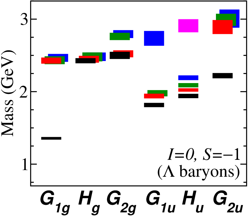


A large effort was undertaken during the last two years to select optimal sets of baryon and meson operators in a large variety of isospin sectors and for zero momentum and non-zero on-axis, planar-diagonal, and cubic-diagonal momenta. Low-statistics Monte Carlo computations were done to accomplish these operator selections using between 50 to 100 configurations on a anisotropic lattice for quark flavors with spacing fm, , and quark masses such that the pion has mass around 380 MeV. Stationary-state energies using the finally selected operator sets are shown in Fig. 1. The nucleon, , , , and baryons were studied, and light isovector and kaon mesons were investigated. Hundreds of operators were studied, and optimal sets containing eight or so operators in each symmetry channel were found. Future computations will focus solely on the operators in the optimal sets.
A comprehensive picture of resonances requires that we go beyond a knowledge of the ground state mass in each symmetry channel and obtain the masses of the lowest few states in each channel. This necessitates the use of matrices of correlation functions. Rather than evaluating a single correlator , we determine a matrix of correlators where are a basis of interpolating operators with given quantum numbers. We then solve the generalized eigenvalue equation to obtain a set of real (ordered) eigenvalues , where . At large Euclidean times, these eigenvalues then delineate between the different masses where . The eigenvectors are orthogonal with metric , and the eigenvectors yield information about the structure of the states.
To study a particular eigenstate of interest with this method, all eigenstates lying below that state must first be extracted, and as the pion gets lighter in lattice QCD simulations, more and more multi-hadron states will lie below the excited resonances. A good baryon-meson operator of total zero momentum is typically a superposition of local interpolating fields at all sites on a time slice of the lattice. In the evaluation of the temporal correlations of such a multi-hadron operator, it is not possible to completely remove all summations over the spatial sites on the source time-slice using translation invariance. Hence, the need for estimates of the quark propagators from all spatial sites on a time slice to all spatial sites on another time slice cannot be sidestepped. Some correlators will involve diagrams with quark lines originating at the sink time and terminating at the same sink time (see Fig. 2), so quark propagators involving a large number of starting times must also be handled.

Finding better ways to stochastically estimate slice-to-slice quark propagators is crucial to the success of our excited-state hadron spectrum project at lighter pion masses. We have developed and tested a new scheme which combines a new way of smearing the quark field with a new way of introducing noise. The new quark-field smearing scheme, called Laplacian Heaviside (LapH), has been described in Ref. [4] and is defined by
| (1) |
where is the three-dimensional covariant Laplacian in terms of the stout-smeared gauge field and is the smearing parameter. The gauge-covariant Laplacian operator is ideal for smearing the quark field since it is one of the simplest operators that locally averages the field in such a way that all relevant symmetry transformation properties of the original field are preserved. Let denote the unitary matrix whose columns are the eigenvectors of , and let denote a diagonal matrix whose elements are the eigenvalues of such that The LapH smearing matrix is then given by Let denote the matrix whose columns are in one-to-one correspondence with the eigenvectors associated with the lowest-lying eigenvalues of on each time slice. Then our LapH smearing matrix is well approximated by the Hermitian matrix Evaluating the temporal correlations of our hadron operators requires combining Dirac matrix elements associated with various quark lines . Since we construct our hadron operators out of covariantly-displaced, smeared quark fields, each and every quark line involves the following product of matrices:
| (2) |
where is a gauge-covariant displacement of type . An exact treatment of such a quark line is very costly, so we resort to stochastic estimation.
Random noise vectors whose expectations satisfy and are useful for stochastically estimating the inverse of a large matrix as follows[6]. Assume that for each of noise vectors, we can solve the following linear system of equations: for . Then , and so that a Monte Carlo estimate of is given by Unfortunately, this equation usually produces stochastic estimates with variances which are much too large to be useful. Variance reduction is done by diluting the noise vectors. A given dilution scheme can be viewed as the application of a complete set of projection operators . Define and further define as the solution of then we have
| (3) |
The use of noise ensures zero variance in the diagonal elements .
The effectiveness of the variance reduction depends on the projectors chosen. With LapH smearing, noise vectors can be introduced only in the LapH subspace. The noise vectors now have spin, time, and Laplacian eigenmode number as their indices. Color and space indices get replaced by Laplacian eigenmode number. Again, each component of is a random variable so that and . Dilution projectors are now matrices in the LapH subspace. In the stochastic LapH method, a quark line on a gauge configuration is estimated using
| (4) |
where the subscripts are compound indices combining space, time, color, and spin, and for a noise vector labelled by index , displaced-smeared-diluted quark source and quark sink vectors can be defined by
| (5) | |||||
| (6) |
Our dilution projectors are products of time dilution, spin dilution, and Laph eigenvector dilution projectors. For each type (time, spin, Laph eigenvector) of dilution, we studied four different dilution schemes. Let denote the dimension of the space of the dilution type of interest. For time dilution, is the number of time slices on the lattice. For spin dilution, is the number of Dirac spin components. For Laph eigenvector dilution, is the number of eigenvectors retained. The four schemes we studied are defined below:
where , and we assume is an integer. We use a triplet (T, S, L) to specify a given dilution scheme, where “T” denote time, “S” denotes spin, and “L” denotes Laph eigenvector dilution. The schemes are denoted by 1 for no dilution, F for full dilution, and B and I for block- and interlace-, respectively. For example, full time and spin dilution with interlace-8 Laph eigenvector dilution is denoted by (TF, SF, LI8). Introducing diluted noise in this way produces correlation functions with significantly reduced variances, yielding nearly an order of magnitude reduction in the statistical error over previous methods. The volume dependence of this new method was found to be very mild, allowing the method to be useful on large lattices. For all forward-time quark lines, we use dilution scheme (TF, SF, LI8), and for all same-sink-time quark lines, we use (TI16, SF, LI8).
Results for three isoscalar mesons are shown in Fig. 3. Such mesons are notoriously difficult to study in lattice QCD, but the new method appears to produce estimates of their temporal correlations with unprecedented accuracy. These plots suggest that evaluating correlation functions involving our multi-hadron operators will be feasible with the stochastic LapH method.


We are currently carrying out these spectrum computations on and anisotropic lattices with spatial spacing fm and aspect ratio , where is the temporal spacing, for pion masses MeV and MeV. The calculations proceed in several steps: (a) generation of gauge-field configurations using the Monte Carlo method; (b) computation of quark sinks for various noises and dilution projectors using the configurations from the first step; (c) computation of the meson and baryon sources and sinks using the quark sinks from the second step; (d) evaluation of the correlators using the hadron sinks; (e) analysis of the correlators to extract the energies. Our results for the QCD stationary-state energies using, for the first time, both single-hadron and multi-hadron operators, should appear soon.
This work was supported by the U.S. National Science Foundation under awards PHY-0510020, PHY-0653315, PHY-0704171, PHY-0969863, and PHY-0970137 and through TeraGrid resources provided by the Pittsburgh Supercomputer Center, the Texas Advanced Computing Center, and the National Institute for Computational Sciences under grant numbers TG-PHY100027 and TG-MCA075017. The USQCD QDP++/Chroma library[7] was used in developing the software for the calculations reported here. We thank our colleagues within the Hadron Spectrum Collaboration.
References
- (1) J. Bulava, R.G. Edwards, E. Engelson, J. Foley, B. Joo, A. Lichtl, H.-W. Lin, N. Mathur, C. Morningstar, D.G. Richards, S. Wallace, Phys. Rev. D 79, 034505 (2009).
- (2) J. Bulava, R.G. Edwards, E. Engelson, B. Joo, H-W. Lin, C. Morningstar, D.G. Richards, S.J. Wallace, Phys. Rev. D82, 014507 (2010).
- (3) C. Morningstar and M. Peardon, Phys. Rev. D 69, 054501 (2004).
- (4) M. Peardon, J. Bulava, J. Foley, C. Morningstar, J. Dudek, R. Edwards, B. Joo, H-W. Lin, D. Richards, K.J. Juge, Phys. Rev. D 80, 054506 (2009).
- (5) S. Basak, R.G. Edwards, G.T. Fleming, U.M. Heller, C. Morningstar, D. Richards, I. Sato, S. Wallace, Phys. Rev. D72, 094506 (2005).
- (6) J. Foley, K.J. Juge, A. O’Cais, M. Peardon, S. Ryan, J. Skullerud, Comput. Phys. Commun. 172, 145 (2005).
- (7) R.G. Edwards and B. Joo, Nucl. Phys. B (Proc. Suppl.) 140, 832 (2005).