August 24, 2026
Superradiance of cold atoms coupled to a superconducting circuit
Abstract
We investigate superradiance of an ensemble of atoms coupled to an integrated superconducting LC-circuit. Particular attention is paid to the effect of inhomogeneous coupling constants. Combining perturbation theory in the inhomogeneity and numerical simulations we show that inhomogeneous coupling constants can significantly affect the superradiant relaxation process. Incomplete relaxation terminating in “dark states” can occur, from which the only escape is through individual spontaneous emission on a much longer time scale. The relaxation dynamics can be significantly accelerated or retarded, depending on the distribution of the coupling constants. On the technical side, we also generalize the previously known propagator of superradiance for identical couplings in the completely symmetric sector to the full exponentially large Hilbert space.
I Introduction
With the advance of experimental quantum information processing, the need to study “hybrid quantum processors” has arisen [1, 2, 3, 4, 5, 6, 7, 8]. In such a processor different physical systems are used in order to exploit their respective advantages, such as long coherence times versus fast processing times, or fast propagation in the case of quantum communication. A natural candidate for a hybrid quantum processor is a system of atoms coupled to superconducting circuits [3]. Circuit-QED schemes are rapidly emerging as a promising new avenue towards scalable quantum computation. These schemes combine the strong coupling and precise control of cavity-QED systems with the scalability of integrated solid state circuits. Nevertheless, the coherence times achieved so far are of the order of a s for transmon qubits [9]. Much longer coherence times are achievable for superpositions of the hyperfine levels of alkali-metal atoms, a fact well known from the design of atomic clocks. Therefore, atoms are predestined as a building block for a quantum memory. The coupling of the hyperfine levels to their environment is through a magnetic dipole transition and thus much weaker than the coupling through an electric dipole. This limits the bandwidth with which information can be transferred to and from such a quantum memory. It is beneficial to use a large number of atoms to store a single excitation [1], as the single photon Rabi frequency that determines the rate of energy exchange scales as with the number of atoms .
Beyond their technical relevance, hybrid quantum processors are also interesting for studying physical effects on a more fundamental level. They allow for easily modifiable parameters, and to reach new parameter regimes, so far inaccessible in traditional quantum optical systems. For example, it has been proposed that the ultra-strong couplings of circuit-QED schemes might allow one to observe the phase transition in superradiance predicted last century by Mallory, and Hepp and Lieb [10, 11, 12]. The existence of such a transition was subject of considerable theoretical debate (see e.g. [13]), culminating in the recent claim that the transition can in principle not be observed in cavity-QED, but should be observable in circuit-QED [14]. For atoms coupled to a superconducting circuit one might envisage to perform precisely controlled experiments on superradiance. Superradiance is a rather complex effect that can include things like mode competitions or beating [15]. It would therefore be desirable to go beyond previous experiments [16, 17, 18, 19, 15] using “traditional” cavity QED in terms of control of different parameters.
In this paper we study superradiance of an ensemble of atoms coupled to an integrated resonant LC circuit. We show that there is indeed a regime in which superradiant behavior is expected. At the same time, additional complications arise due to variations in the coupling constants, which are fundamentally related to the small size of the integrated LC circuit. Most of this paper is therefore dedicated to the study of the effects of inhomogeneous coupling constants on superradiance. So far the study of superradiance has been almost entirely limited to homogeneous coupling constants, and/or initial states that are fully symmetric under all permutations of atoms. We develop a general theoretical framework that allows one to deal with such inhomogeneities. Based on perturbation theory in the inhomogeneity, this framework starts with the construction of a semiclassical solution of the superradiant master equation in the entire exponentially large Hilbert space for the homogeneous case.
II Model
II.1 Physical system
We consider atoms that are, on the time scale of the experiment, held at fixed positions close to an -circuit (see Fig. 1).

We assume that a single atomic transition is in resonance with a single mode of the cavity. To be specific, we are particularly interested in an ensemble of 87Rb atoms trapped and cooled in a dipole trap in close vicinity (a few m) of the surface of the -circuit. Neutral 87Rb has a hyperfine split ground state with total angular momentum and . The hyperfine splitting between the states with and is GHz [20, 21]. Without an external magnetic field, the Zeeman sublevels with -component of the total angular momentum are degenerate. We will focus on the situation where an additional small static -field in the direction is applied that splits the degenerate hyperfine states, and defines the quantization axis for the atoms. Neglecting the magnetic dipole moment of the nucleus, and for small magnetic field strength , the magnetic moment of an atom is given by
| (1) |
where and are the -factor and total electron angular momentum vector, respectively, and is the Bohr magneton (with and the electron charge and mass).
We consider a simple current carrying loop with inductance , that is part of a resonant circuit with frequency . The resonator can be treated as a harmonic oscillator with Hamiltonian . The creation and annihilation operators and are related to the current in the circuit by . That current gives rise to a magnetic field
| (2) |
where is a dimensionless mode function with components depending on the geometry of the circuit, a typical linear dimension of the circuit, and the magnetic constant. The magnetic moment of a single atom at position couples to the magnetic field through the interaction Hamiltonian , which can be written in the basis as
| (3) |
Starting in , the only non-vanishing resonant transition due to a from the circuit oscillating at angular frequency is then to with matrix element . Note that to first order in the additional static -field, and are not shifted by the field. In the interaction picture with respect to the free Hamiltonian , the operators and acquire time-dependent phase factors and , respectively, which justifies the use of a rotating wave approximation. The interaction Hamiltonian for atoms at position then takes the familiar form
| (4) |
with ,
| (5) |
and is the Pauli lowering operator for atom .
In Fig. 2 we show for an circuit in the form of a square loop of size m in the –plane, and a 87Rb atom located at position on the symmetry axis perpendicular to the loop, where the origin of the coordinate system is located at the lower left corner of the square, and the center of the square is .
(a) 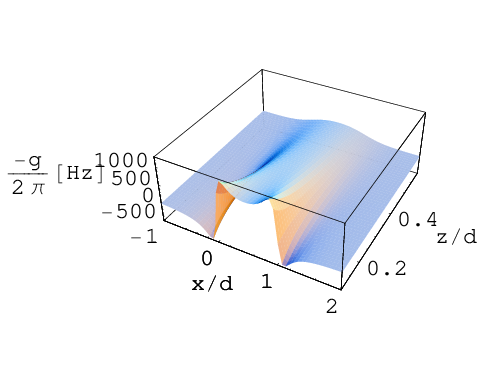 (b)
(b) 
The coupling for an atom at with m is Hz. For m, it increases to Hz, whereas at m, we have Hz. We consider a thermal cloud of atoms confined by a 3D harmonic trap with trapping frequencies (), centered at with atom positions taken as classical variables, distributed according to the probability density . Here,
| (6) |
is the thermal equilibrium distribution at temperature for a one-dimensional harmonic oscillator of frequency and atomic mass , with , , and (see e.g. problem 2.6 in [22]). From we obtain the distribution of coupling constants
| (7) |
where the integration is over the entire space . Examples of are shown in Fig. 2. We see that even at temperatures as low as K, relatively large trapping frequencies of 1 kHz in all directions, and a loop size of m, the coupling constants can easily vary by 50% or more. For higher temperatures K, long tails in with substantially larger absolute coupling constants appear due to atoms close to the loop. For K, the spread in position becomes comparable to , and many atoms are therefore located “outside” the loop, leading to coupling constants with opposite sign, and a distributed around an average value close to zero. It is therefore clear that the consequences of the inhomogeneity of the coupling constants need to be investigated.
II.2 Superradiance
Superradiance is a collective emission process of two–level atoms resonantly coupled to a single mode of a resonator (under suitable conditions it can even be observed without a resonator, see [15]). It is observed under several conditions [23, 15]: 1.) The temperature of the electromagnetic environment must be much smaller than the level spacing of the atoms, such that photons only leave the resonator, whereas the entering of thermal photons can be neglected, and 2.) the resonator must be rather leaky. More precisely, if all atoms couple identically to the resonator, one should have , where is the single photon escape rate from the resonator, and denotes the single atom spontaneous emission rate. The latter is, in our case of hyperfine levels of 87Rb atoms, entirely negligible. Photon escape from the resonator is due to the finite quality factor, , of the circuit. factors of up to have been achieved for superconducting circuits [24], leading to of the order of several kHz. For such a high-quality resonator, and the typical coupling constants of a few 100 Hz calculated in section II.1, the number of atoms would be restricted to about 100. However, the quality factor of the circuit can be easily decreased (e.g. by increasing the temperature, or using a more lossy substrate), or the distance of the atoms from the circuit can be increased, thus reducing the coupling constants. One can therefore accommodate much larger numbers of atoms. Below we also derive a lower bound on the number of atoms for the validity of the present analysis.
Under the above conditions, and the assumption of weak inhomogeneity with , the superradiant master equation in the rotating frame
| (8) |
can be derived. Here, represents the reduced density matrix describing the hyperfine states of the atoms, after tracing out the mode of the resonator and its electromagnetic environment. As mentioned above, the external state of the atoms is taken as a classical degree of freedom, uncorrelated from the internal states of the atoms, and with the atoms at fixed positions on the time scale of the experiment. The rate is linked to and by . The are collective ladder operators, related to the single-atom Pauli matrices in the Hilbert space of the two levels participating in the resonant transition by
| (9) |
where denotes a dimensionless coupling strength, and is a reference coupling strength (which might be chosen e.g. as the average coupling constant over all atoms). For later use we also define . The derivation of Eq. (8) follows closely the calculation in [23]. One checks that in the case of weak asymmetry the derivation in [23] remains valid if the pseudo-angular momentum operators used in [23] are replaced by defined by Eq. (9).
The homogeneous situation, with identical coupling constants, has the tremendous advantage of the dynamics remaining restricted to a single irreducible representation (irrep) of with angular momentum quantum number . In particular, if one starts with all atoms excited, or any other state fully symmetric under permutation of atoms, then is the maximum possible (pseudo-)angular momentum number. Thus, instead of having to track states, we only have to deal with states. In the following we will consider the situation of weak inhomogeneity and assess the effect of the deviations to first order perturbation theory. We also introduce a rescaled dimensionless time, , , which means that everything will be expressed in terms of the classical time scale of the system [25]. In particular, probabilities are known to propagate on a time scale , whereas macroscopic coherences in superradiance normally decay on the much shorter time scale .
Before studying the superradiance dynamics, let us determine the parameter regime in which we expect our approximation of atoms with fixed classical positions to be valid. The one-atom reduced density matrix of a non-interacting atom gas in thermal equilibrium in a 1D harmonic oscillator in position representation is given by
| (10) |
We see that the coherences decay on a length scale , which is given by and [22]. Quantum effects in the external degree of freedom of the atoms can be neglected if , the harmonic oscillator length scale of confinement of the atoms (and correspondingly for directions ). This implies , which leads to roughly . Thus, for trapping frequencies of the order of 1 kHz treating the atom positions classically is reasonable down to temperatures of order 100 nK, and for trapping frequencies of order 100 Hz even 10 nK still means that the atom positions are essentially classical variables.
A second restriction arises from the requirement of fixed atom positions on the time scale of the experiment. The typical thermal velocity in the -direction of an atom follows from the equipartition theorem, . A typical time scale of an experiment is given by the decay time of the superradiant pulse, . During that time the atom should move at most a distance much smaller than , the typical length-scale on which changes. This leads to a lower bound on the number of atoms, . Together with the upper bound for the existence of superradiance, one obtains an allowed range of permissible values of . Requesting an upper bound much larger than the lower bound leads to the requirement 8 mK in the case of 87Rb. This leaves a comfortable range of the Rb temperatures for resonators with a quality of order 1000, corresponding to MHz. Using temperatures close to the lower bound considered above will have the advantage that one may even record many runs with the same atom positions, and thus separate quantum fluctuations from the superradiant dynamics (e.g. waiting time distributions after initial excitation) from fluctuations due to changing coupling constants. As an example, for Hz, Hz, we have the requirement . At a temperature of K, the thermal speed of the Rb atoms is of the order 1 cm/s, and for m, we need .
We now proceed with the analysis by rewriting (8) as
| (11) | |||||
| (12) | |||||
| (13) | |||||
| (14) | |||||
| (15) |
where in the last step we have neglected the terms of order . We have introduced a book keeping parameter , assuming that is small compared to . In the end we will set . We also expand in terms of ,
| (16) |
To order , we retrieve the original Lindblad master equation
| (17) |
with initial condition . To first order, , we get
| (18) |
The formal solution of (18) is given by
| (19) |
It describes the usual situation of propagating the initial density matrix with the “free” propagator corresponding to the homogeneous case up to a time , then have the perturbation act at time , and then continue with the “free” propagation till the end of the time interval. The free propagator has been well studied, and in particular very precise semi-classical expressions exist, both for the propagation of the probabilities and for the coherences — but only for relevant for the homogeneous case [26, 23, 27, 28, 29, 25]. Here, we have the added complication that does not conserve , as is by definition not symmetric under exchange of atoms. We therefore need a more general expression for the free propagator for the time interval . We will derive here a free propagator valid in the entire dimensional Hilbert space, represented in all irrep components, by generalizing the method in [29] that allows one to connect the propagator for coherences to the one for probabilities. Secondly, we will obtain explicit expressions for the matrix elements of in and between different irreps. Taken together, this will allow the construction of the full propagator according to Eq. (18).
The irreducible representations of can be constructed by adding one spin-1/2 after another. When adding a new spin, the available values of total angular momentum , can either increase or decrease by . Therefore, for , there are many ways to get to a particular value for given number of atoms . These different ways lead to different degenerate irreps for the same . A quantum state must accordingly be labeled not only by the total angular momentum and (), but also by additional quantum numbers , which distinguish different irreps with the same . We may consider as the label of a path on the lattice of allowed combinations that leads to the value of at hand. We thus have states that are eigenstates of and with eigenvalues and , respectively, which we can use to represent . It will turn out that to first order perturbation theory, one needs only the irreps with and . This is a consequence of the fact that only contains tensor operators of rank 1 and 2.
III Superradiance for homogeneous couplings in the entire Hilbert space
It can be shown that the superradiant master equation (8) with homogeneous couplings conserves both and , i.e.
| (20) |
with . Conservation of has been known from the early days of superradiance and allowed a formulation of the problem in the irrep. Conservation of can be shown by complete induction. Below we will consider the situation of two sub-ensembles of atoms, each of which is homogeneous on its own. In that case we will see that conservation of also follows from selection rules encoded in the angular momentum algebra.
It is worthwhile to express the matrix elements of as
| (21) |
where is a “center of mass” quantum number, , and for a matrix element . A value different from zero, , or signifies a coherence. The quantum numbers and are simultaneously integer or half-integer. In order to render the notation less cumbersome, we denote the set of quantum numbers collectively as . We can then write Eq. (17) as
| (22) |
and see that probabilities and coherences do not mix under time evolution, nor do coherences defined through different combinations of , and . The coefficients and are independent of , and are defined as
The master equation can be solved with the help of the propagator , which is non-diagonal now only in the quantum numbers . We can thus write
| (23) |
where we have used that the propagator does not depend on . The sum over runs over all values from to in steps of 1, and is restricted to the same interval. These bounds follow from requesting and . The initial condition is . The equation can be solved exactly by Laplace transformation,
| (24) |
which leads to the recursion relation
| (25) |
The solution
| (26) |
valid for all , has poles at . It remains to perform the inverse Laplace transform,
| (27) |
where needs to be chosen larger than the real part of all poles. Unfortunately, for large , there are many poles, which makes the inverse Laplace transform cumbersome. However, we can relate the propagator for coherences to the propagator of probabilities [29] by noting that
| (28) | |||||
| (29) | |||||
| (30) |
Once we shift the integration variable in Eq. (27) by and define
| (31) |
we find
| (32) |
where is the propagator of probabilities. A precise semiclassical approximation for can be found in [29, 25]. We thus have through Eq. (32) immediate access to a propagator in the entire exponentially large Hilbert space.
The independence of on implies that coherences with between irreps with different , but the same , decay just as slowly as the probabilities within any irrep with the same . This constitutes another example of slowly decohering Schrödinger cat states, with which the theory of superradiance is rich [30]. The physical reason for this is that the Lindblad operator is totally symmetric under permutation of atoms, and therefore cannot make transitions between irreps with different values of . Previously known examples of slowly decohering Schrödinger cat states in superradiance include superpositions of angular momentum coherent states in the irrep that are symmetric with respect to the equator . They also decohere just as slowly as the corresponding probabilities. Furthermore, there is a well known decoherence free subspace (DFS) of dimension that contains the states of all irreps in which all superpositions, as macroscopic or entangled as they may be, are decoherence free under this collective decoherence process [31].
IV Two subsystems
The superradiance process depends on all individual coupling constants. To simplify the problem at hand, let us look at only two sub-ensembles with and atoms (), and coupling constants and , respectively. While this exact distribution of coupling constants may not be very realistic, one may hope to develop an idea of the effects of inhomogeneity in this situation that may still be qualitatively correct for more complicated distributions of couplings, and to find a solution that is still analytically tractable. For an arbitrary distribution of coupling constants one may choose to adjust , and to the first three nontrivial moments of the distribution. The results are
| (33) |
and
| (34) |
Here, , etc. We assume that is big enough such that rounding to the next integer or half integer value for does not lead to a significant change. The advantage of working with just two different couplings is that explicit analytical formulas for can be obtained. We define the eigenstates of and for . The basis functions which are eigenstates of , , , and , will be used to represent the state of the whole system. The symmetry label corresponds then to the pseudo-angular momentum quantum numbers , for the two sub-ensembles.
For given couplings and , we have . We also introduce the ladder operators , , , and in the two subsystems, defined as
| (35) |
in Eq. (15) then becomes
| (36) |
We then need to calculate the matrix elements of ,, and , in basis states . The results can be found in the Appendix. All these matrix elements are real. The expressions for and are obtained from those for and simply by exchanging , which evidently leaves the expressions unchanged if . Equation (15) then tells us that for , for any that is symmetric under the exchange of the two subsystems, . This means that to first order perturbation theory the effect of the inhomogeneity in the couplings vanishes exactly if the two sub-ensembles contain the same number of atoms and the initial state is in the irrep.
IV.1 Full propagator
Let us consider the case of an initially pure state, with support only in the irrep with . Since we start off with a totally symmetric state, the initial state is also totally symmetric under permutations in each sub-ensemble, and we have therefore initially , . To zeroth order we find
| (37) |
with . The first order correction to the density matrix can be written as
| (38) |
with a propagator defined as
The sums over are restricted such that . We have introduced the representation of in the irrep states,
| (45) | |||||
With these expressions we can now evaluate any time dependent expectation value.
V Results
V.1 Short time behavior of population inversion
The population inversion is given by . To zeroth order we have
| (46) | |||||
and to first order
| (47) |
The propagator involves the matrix elements now only for , and . Since , the summation over in (47) is restricted to (see the remarks after Eq. (A.2)). Moreover, it is possible to obtain closed, compact expressions for these matrix elements, at least in the case of , which is relevant if the initial state is a Dicke state . To this end it is useful to consider the three cases and separately.
- 1.
For , matrix elements of and of contribute, and we find
(51) - 2.
For , only contributes, due to the Kronecker-deltas that come with . We obtain
(55) where in the last step we have used such that the prefactor is symmetric under .
- 3.
For , we find immediately that this contribution vanishes, as cannot change by more than one unit, and for the term the prefactor is again zero due to the Kronecker-deltas.
The only contribution to stems therefore from the original fully symmetric irrep with . Experimentally, the most relevant situation is a fully excited initial state , which can be achieved e.g. by optical pumping with external laser light that acts on all atoms in the same way. In this case, one obtains the explicit result for the first order correction,
| (56) | |||||
Equation (56) is one of the main results of this paper. It shows once more that vanishes for . Moreover, all dependence on is in the prefactor , such that for given it is sufficient to calculate for any , and then rescale accordingly.

Figure 3 shows calculated from Eq. (47) and from exact diagonalization of the full propagator for a small number of atoms and for very small , such that . The agreement is perfect. We see that vanishes at , and then decreases as function of time, before increasing again. This implies a more rapid initial decay of the population inversion for than for the homogeneous case. As the loss of atomic excitation goes along with an increase of the photon number in the cavity, superradiance is accelerated by the inhomogeneity. Note that together with means that there are more atoms with the larger of the two coupling constants, such that one indeed expects an acceleration of superradiance compared to the homogeneous case. For , changes sign, and superradiance slows down.
Figure 3 also shows that for sufficiently large times, vanishes. This can be understood from Eq. (56), as for large the two free propagators under the integral cannot be simultaneously substantially different from zero for the combinations of indices that appear. As a consequence, the effect of inhomogeneity on the average value of for is at most a quadratic function of , even for (see also next subsection). This means that there is a finite time after which first order perturbation theory becomes inadequate, and higher order corrections will dominate.
The time-independent factors in Eq. (56) scale proportional to for . However, the integration over brings down a factor (see Eq. (32), and Eq. (4.56) in [31]). The free propagators are of order 1, such that scales as as it should, and first order perturbation theory remains meaningful for large . This means that it is enough to calculate for moderate values of , as it will saturate as function of .
V.2 Incomplete Relaxation
Another important consequence of inhomogeneous coupling constants that can be observed even for a very small number of atoms is incomplete relaxation (neglecting spontaneous emission — see the remarks in sec.II.1). It is well known that for fully -symmetric superradiance there is a large decoherence free subspace (DFS) [31, 32] containing dark states for even (of for odd) . These states, defined through , can trap the dynamics, in the sense that if such a state is reached, the superradiant dynamics is switched off and further evolution is only possible through competing mechanisms neglected so far. The simplest example is given for with two DFS states. If we denote the two hyperfine states involved as and , the DFS states are the ground state and the “singlet” state . In the singlet state both atoms together contain one photon, but destructive interference prevents the transfer of the photon from the atoms to the cavity (from where it would escape). A way of reaching that state is to start in an initial state , which in half the cases will emit a photon, but in the other half get trapped in the singlet state [33]. This constitutes a simple way of preparing an entangled state through a decoherence (and even dissipation) mechanism: If no photon leaves within a time given by max( 1/, 1/ ), the system is with high probability in the singlet state.
More generally, for perfect symmetry, the DFS states are the (typically highly degenerate) ground states of all the irreps with (assuming even). If the symmetry is broken, the DFS does not disappear, but rather gets rotated in Hilbert space. For example, for , and real coupling constants and , the singlet is replaced by a state , which is still annihilated by , the new collective Lindblad-operator. This parametric dependence of the DFS on a system parameter is at the basis of “decoherence-enhanced measurements” [34, 35], which allow precision measurements with Heisenberg-limited sensitivity while using initial product states.
With perfect symmetry, an initially fully excited state with remains in that irrep and relaxes to the ground state, without ever reaching a nontrivial DFS state, which only exists for . However, when the symmetry is broken, is no longer conserved, and nontrivial DFS states can be reached, resulting in the trapping of the population. Since the first order correction to vanishes for large , the trapping effect is beyond reach of the perturbation theory developed above. We therefore resort to a numerical approach by simulating the stochastic Schrödinger equation (SSE) that unravels Eq. (11). The SSE is given by
| (57) | |||||
| (58) | |||||
| (59) |
is a Wiener process with average zero and variance , and [36]. When averaging over a large number of realizations of the stochastic process one obtains a numerically exact solution of the master equation. In principle this can be done even for arbitrary coupling constants, but we stay with the situation of two different subsystems. A drawback of the numerical approach is that it is limited to a small number of atoms.
Figure 4 illustrates the incomplete relaxation in the inhomogeneous case for typical realizations of the stochastic process from Eq. (57). For , superradiance proceeds down to the ground state, whereas for the trajectories can get trapped at a random finite value . The statistical analysis of these final values (we take , as the trajectories typically have converged at that time) leads to the histograms shown in the same figure, obtained from runs of the SSE, , and . For , the histogram is a -peak at , as the superradiant relaxation proceeds to the total ground state. For , a -peak at arises. This is due to the fact that in this case the second set of atoms has coupling constants zero. Therefore, these atoms remain excited, whereas the atoms in the first set decay to the ground state, such that in the end half of the excitation remains in the system, resulting in . In general, for the final value for is given by . For intermediate values of , the histogram rapidly broadens and shifts to larger values of with increasing .
(a)  (b)
(b) 
Figure 5 shows the average value of for large () as a function of obtained from these realizations and the standard deviations (as errorbars) for , , and for , . Initially we see quadratic behavior, which arises from the vanishing of for or .

VI Conclusions
We have presented a thorough analysis of the effect of superradiance of cold atoms coupled to a superconducting on-chip -resonator. Under realistic conditions we demonstrated a parameter regime in which superradiance should be observable. We have analysed the effect of inhomogeneous couplings on the superradiance process by perturbation theory in the inhomogeneity, and numerical simulations. By dividing the sample into two subensembles, with different atom numbers and coupling constants, we can model the inhomogeneous coupling. Our results show that superradiance may be accelerated or slowed down compared to the homogeneous case, depending on the distribution of coupling constants. The first order correction in the inhomogeneity vanishes for all observables in the case of two sub ensembles containing the same number of atoms. For large times, inhomogeneous coupling constants can lead to population trapping in random decoherence free states, and we have provided numerical results for the population inversion starting from a initially fully excited state. The first order correction to the final average population inversion vanishes in this case, such that the change of that quantity is at most quadratic for small inhomogeneity.
Acknowledgments: DB thanks the Joint Quantum Institute (University of Maryland and NIST) for hospitality when this work was initiated, and CALMIP (Toulouse) for the use of their computers.
Appendix A Evaluation of matrix elements of angular momentum operators
We use two different ways of calculating matrix elements of angular momentum operators in the joint basis : i.) Decoupling the basis states into single angular momentum basis states using Clebsch-Gordan coefficients and ii.) using the Wigner-Eckart theorem.
A.1 Decoupling into single angular momentum basis states
A straight forward way of obtaining the matrix elements of and is to decouple
| (60) |
where the coefficients are Clebsch-Gordan coefficients. Then apply the desired operator, and couple the states back together using the inverse transformation,
| (61) |
Since the are symmetric under permutation of the atoms in subsystem , they conserve , such that the matrix elements are all diagonal in the index . We find
Another derivation which in the end gives closed analytical expressions is based on the Wigner-Eckart theorem.
A.2 Wigner-Eckart theorem
Let us consider momentarily a single angular momentum (i.e. with Hilbert space dimension spanned by basis states which form a simultaneous eigenbasis of and ). The Wigner-Eckart theorem states that the matrix elements of an irreducible tensor operator which transforms according to the irrep of with , i.e. like a state , is given by
| (74) |
where is a reduced matrix element that does not depend on the magnetic quantum numbers , or [37]. In practice one calculates these by using the Wigner-Eckart theorem backwards for a simple operator whose matrix elements are known. There is just one scalar tensor operator that can be formed from the components of , . Tensor operators of rank 1 (i.e. a vector) are formed by the components of . We have
| (75) |
Higher order tensor operators of rank up to can be formed from the product of lower rank tensors , ,
| (76) |
One particular example is a tensor formed by the Cartesian product of the components of the vector operator () introduced above, which we denote as , and which reads
| (77) |
The Clebsch-Gordan coefficients limit the possible values of to . We can invert this relation and obtain the reduction of a product of irreducible tensor operators into a sum of irreducible tensor operators,
| (78) |
With the help of this equation we can reduce the product into its irreducible components,
| (79) |
Note that . This relation can be
shown component by component using Eqs. (77,75), and the
commutation relations of the angular momentum operators.
Now consider a composite system of two (physical or pseudo-) angular momenta and . We distinguish the operators acting on subsystem as before by a superscript, . The reduced matrix elements of an operator which acts only subsystem 1, , can be related to the ones in subsystem 1 alone according to
| (80) |
where the symbol is related to Wigner’s -symbol by
| (81) |
see Eq. (5.9) in [37]. From (79,80) we obtain
| (85) | |||||
It remains to calculate the reduced matrix elements. Brink and Satchler [37] (p.51ff) give for a single angular momentum . Using this in the Wigner Eckart theorem, sandwiched between states and gives for a single angular momentum
| (95) |
Similarly, from we find
| (96) |
and
| (97) |
Finally, one can show that by applying (77), and the Wigner-Eckart theorem tells us that hence
| (98) |
and thus
| (102) | |||||
We have checked numerically up to and all combinations of (with ) that Eqs. (A.2,102) give exactly the same results as Eqs. (A.1,A.1), respectively. Eqs. (A.2,102) have the advantage of avoiding an additional sum, and of leading to explicit expressions for the case relevant for the calculation of , as we demonstrate in Results section. Furthermore, the selection rule is evident from these equations, as otherwise the Clebsch-Gordan coefficients vanish.
References
- [1] L. Duan, M. D. Lukin, J. I. Cirac, and P. Zoller, Nature 414, 413 (2001).
- [2] D. Petrosyan and M. Fleischhauer, Phys. Rev. Lett. 100, 170501 (2008).
- [3] D. Petrosyan, G. Bensky, G. Kurizki, I. Mazets, J. Majer, and J. Schmiedmayer, Phys. Rev. A 79, 040304(R) (2009).
- [4] P. Rabl, D. DeMille, J. M. Doyle, M. D. Lukin, R. J. Schoelkopf, and P. Zoller, Phys. Rev. Lett. 97, 033003 (2006).
- [5] A. S. Sørensen, C. H. van der Wal, L. I. Childress, and M. D. Lukin, Phys. Rev. Lett. 92, 063601 (2004).
- [6] L. Tian, P. Rabl, and P. Zoller, Phys. Rev. Lett. 92, 247902 (2004).
- [7] J. Verdu, H. Zoubi, C. Koller, J. Majer, H. Ritsch, and J. Schmiedmayer, Phys. Rev. Lett. 103, 043603 (2009).
- [8] M. Wallquist, K. Hammerer, P. Rabl, M. Lukin, and P. Zoller, Physica Scripta T137, 014001 (2009).
- [9] A. A. Houck, J. A. Schreier, B. R. Johnson, J. M. Chow, J. Koch, J. M. Gambetta, D. I. Schuster, L. Frunzio, M. H. Devoret, S. M. Girvin, et al., Physical Review Letters 101, 080502 (2008).
- [10] K. Hepp and E. H. Lieb, Annals of Physics 76, 360 (1973), ISSN 0003-4916.
- [11] W. R. Mallory, Physical Review A 11, 1088 (1975).
- [12] G. Chen, Z. Chen, and J. Liang, Physical Review A 76, 055803 (2007).
- [13] K. Rzazdotewski, K. Wódkiewicz, and W. Zdotakowicz, Physical Review Letters 35, 432 (1975).
- [14] P. Nataf and C. Ciuti, Nat Commun 1, 72 (2010).
- [15] M. Gross and S. Haroche, Phys. Rep. 93, 301 (1982).
- [16] N. Skribanowitz, I. P. Herman, J. C. MacGillivray, and M. S. Feld, Phys. Rev. Lett. 30, 309 (1973).
- [17] M. Gross, C. Fabre, P. Pillet, and S. Haroche, Phys. Rev. Lett. 36, 1035 (1976).
- [18] M. Gross, J. M. Raimond, and S. Haroche, Phys. Rev. Lett. 40, 1711 (1978).
- [19] M. Gross, P. Goy, C. Fabre, S. Haroche, and J. M. Raimond, Phys. Rev. Lett. 43, 343 (1979).
- [20] S. Penselin, T. Moran, V. W. Cohen, and G. Winkler, Phys. Rev. 127, 524 (1962).
- [21] S. Bize, Y. Sortais, M. S. Santos, C. Mandache, A. Clairon, and C. Salomon, EPL (Europhysics Letters) 45, 558 (1999).
- [22] W. Schleich, Quantum Optics in Phase Space (Wiley-VCH Verlag Berlin GmbH, Berlin, Germany, 2001).
- [23] R. Bonifacio, P. Schwendiman, and F. Haake, Phys. Rev. A 4, 302 (1971a).
- [24] A. J. DiNardo, J. G. Smith, and F. R. Arams, J. Appl. Phys. 42, 186 (1971).
- [25] P. A. Braun, D. Braun, and F. Haake, Eur. Phys. J. D 3, 1 (1998a).
- [26] G. S. Agarwal, Phys. Rev. A 2, 2038 (1970).
- [27] R. Bonifacio, P. Schwendiman, and F. Haake, Phys. Rev. A 4, 854 (1971b).
- [28] R. J. Glauber and F. Haake, Phys. Rev. A 13, 357 (1976).
- [29] P. A. Braun, D. Braun, F. Haake, and J. Weber, Eur. Phys. J. D 2, 165 (1998b).
- [30] D. Braun, P. A. Braun, and F. Haake, Proceedings of the 1998 Bielefeld Conference on ”Decoherence: Theoretical, Experimental, and Conceptual Problems”, Lect. Notes Phys. 538, 55 (2000).
- [31] D. Braun, Dissipative Quantum Chaos and Decoherence, vol. 172 of Springer Tracts in Modern Physics (Springer, 2001).
- [32] A. Beige, D. Braun, and P. L. Knight, New Journal of Physics 2, 22.1 (2000).
- [33] M. B. Plenio, S. F. Huelga, A. Beige, and P. L. Knight, Phys. Rev. A 59, 2468 (1999).
- [34] D. Braun and J. Martin, Decoherence-enhanced measurements, eprint arXiv:0902.1213v2.
- [35] D. Braun and J. Martin, Collectively enhanced quantum measurements at the Heisenberg limit, eprint arXiv:1005.4443.
- [36] H.-P. Breuer and F. Petruccione, The Theory of Open Quantum Systems (Oxford University Press, 2006).
- [37] D. Brink and G. Satchler, Theory of Angular Momentum (Clarendon Press, Oxford, 1968).