Structure of and threshold behavior of scattering
Abstract
The scattering length and effective range of the channel are studied in order to characterize the strangeness meson-baryon scattering and the resonance. We examine various off-shell dependence of the amplitude in dynamical chiral models to evaluate the threshold quantities with the constraint at the threshold. We find that the threshold parameters are important to the structure of the resonance and provide further constraints on the subthreshold extrapolation of the interaction.
1 Introduction
The hyperon resonance has strangeness and isospin , and is located just below the threshold of . Because is considered to be the quasi-bound state of the channel, the structure of is one of the very important issues of recent hadron physics, especially to understand -nucleon and -nucleus interactions. At the same time, is a resonance decaying to the channel with by the strong interactions. Thus, for the nature of , dynamics of both and is important and gives essential contributions.
The resonance has been considered as a dynamically generated state in meson-baryon scattering for a long time before establishment of QCD, while the possibility of the with some three-quark components originated in quark-model viewpoint has been also discussed. The first dynamical investigation of in terms of meson and baryon degrees of freedom was performed by Dalitz and Tuan [1]. There and scattering amplitudes were calculated in a coupled-channels approach and was obtained as a quasi-bound state of . It was also confirmed in a modern point of view that can be predominantly described by meson-baryon components in a coupled-channels approach based on chiral dynamics [2] (chiral unitary model), which successfully reproduced in meson-baryon dynamics [3, 4, 5, 6, 7, 8, 9, 10, 11, 12]. A phenomenological approach also described as a quasi-bound state of [13], in which an effective interaction of was derived so as to reproduce the scattering length and the mass and width of as 1405 MeV and 40 MeV, as suggested by the Particle Data Group (PDG).[14] Concerning the amplitude above the threshold, this effective potential is essentially consistent with the one extracted from the chiral unitary approach [15], although the phenomenological model provides quantitatively stronger interaction than the chiral potential in the region far below the threshold. Thus, there are uncertainties about the theoretical extrapolation of the interaction below the threshold.
Another recent finding is that is composed by two resonance states appearing around energies which have different coupling nature to the and channels [5, 9, 16, 17]. According to Ref. \citenJido:2003cb, one state which dominantly couples to the state is located at 1420 MeV instead of nominal 1405 MeV with a narrower width, while the other state couples strongly to the channel and appears around 1390 MeV with a wider width. Because of the dominant coupling to the , the higher pole is more relevant to the -nucleus interaction [15]. Thus, it is extremely important to reveal the resonance position in the channel. This double pole structure of also leads to the feature that the resonance spectra depend on its production mechanism [9, 18, 19, 20, 21]. For observation of spectra below the threshold, an old bubble-chamber experiment in gave a hint of the resonance position at 1420 MeV [22]. A recent theoretical analysis based on the chiral unitary approach [21] confirmed that the production is initiated by the channel in the , and was able to reproduce the production cross section and the shape of the experimental observed spectrum. Further detailed experimental information of the spectrum will be obtained in ongoing/forthcoming experiments at Jefferson Laboratory [23], GSI [24], and J-PARC. [25]
Recent theoretical investigations based on coupled-channels approaches in chiral dynamics suggested the double pole structure of . Nevertheless, the position of the lower pole is dependent on the details of the model parameters, as discussed in Ref. \citenHyodo:2007jq. Moreover, Ref. \citenIkeda:2010tk shows that the use of the approximate energy independent potential also changes the pole position drastically. Indeed, since the pole position of the higher state is strongly constrained by observed scattering and hydrogen experiments, the theories provide very similar pole positions around 1420 MeV with narrow widths within the framework of several chiral unitary models. However, due to lack of experimental data, the properties of the lower state are less controlled in theoretical studies. Hence the pole position of the lower state has model dependence even in similar models constructed by the same concept. The dynamics, including the nature of the lower pole, may be important in kaonic nuclear few-body systems. A possible quasibound state of was proposed in 60’s [27], and recent theoretical investigations concluded that the system has a quasibound state with a large width [13, 28, 29, 30, 31, 32, 26], and the theoretical predictions of the energy and width scatter over a wide range. Although part of the ambiguity in the model prediction has been attributed to the treatment of the three-body dynamics [32] and the energy dependence of the interaction [26], it is obvious that the present experimental database does not completely constrain the - interaction. Since the threshold is located at 100 MeV below the threshold, if is bound in few-body systems with a large binding energy, the coupling to the channel is essential to understand the properties of the quasibound state.
In this paper, we discuss threshold behavior of the scattering11 1 A preliminary discussion was given in Ref. \citenJido:2010ag., emphasizing its importance in a context of the resonance in chiral dynamics. For the physics of , it is certainly necessary to have theoretical descriptions of and dynamics applicable for the energy region between their thresholds, which is as wide as 100 MeV. The nature and position of the pole singularity (bound state, virtual state, or resonance) around the threshold22 2 Here we investigate the coupled-channels scattering amplitudes below the threshold. Thus, we search the poles in the physical sheet of the complex energy plane and classify the poles in terms of the Riemann sheets for the channel. is an important issue. Because chiral symmetry indicates that the -wave diagonal interaction at low energy with is strongly attractive, a pole singularity may be produced at least somewhere, probably close to the threshold, in the complex energy plane. It is known that the leading order calculations of the pion-nucleon and pion-pion scattering lengths in the chiral perturbation theory work well within 20% accuracy. Thus, it is an interesting question whether it is also the case for the scattering length for the channel with . To clarify the nature of the dynamics, we calculate the scattering length and the effective range in various models of the and coupled channels in which different ways of solving Lippmann-Schwinger equation are applied in the isospin limit. Finally, we conclude that the scattering length and effective range give us new and essential information of the - dynamics between their thresholds and the resonance. We discuss the general relationship between the scattering length and the effective range with the pole singularity around the threshold in Appendix.
2 Two channel models of - scattering
We discuss the threshold behavior of the amplitude with in connection with the resonance appearing below the threshold. To describe the scattering amplitude and the resonance, it is essential to treat both and channels simultaneously in a coupled-channels approach. Here we consider simple models of coupled and channels with based on chiral effective theory. The interaction kernel is given by the Weinberg-Tomozawa interaction and we solve coupled-channel Lippmann-Schwinger equation with this interaction kernel. In our model, there are two adjustable parameters which come from the regularization of the Lippmann-Schwinger equation. These parameters are determined by the scattering length with . We shall also compare different theoretical schemes for solving Lippmann-Schwinger equation for the - coupled system.
2.1 Framework of the models
Let us start with Lippmann-Schwinger equation for the -operator of the and channels with :
| (1) |
where is the scattering energy in the center-of-mass frame, is the interaction kernel, and is the free two-body Green operator. We solve the Lippmann-Schwinger equation in the center-of-mass system. Inserting complete sets of the meson-baryon states, we obtain the Lippmann-Schwinger equation for the -matrix element:
| (2) | |||||||
where and are final and initial meson (baryon) momenta with the channel indices , respectively. In general, we need off-shell interaction kernel and -matrix element to solve Eq. (2). In this equation, the two-body meson-baryon state is normalized as where with the baryon mass , the baryon energy , the meson energy and the meson mass . The on-shell meson (baryon) momentum is given by
| (3) |
We fix the interaction kernel based on the chiral effective theory. At the leading order of the chiral expansion for the -wave scattering, we take so-called Weinberg-Tomozawa interaction given by
| (4) |
where and are channel indices of () and (), is the meson momentum for channel and is fixed to the on-shell energy in the center-of-mass system, is the meson decay constant, is the Dirac spinor for the baryon and is the coupling strength which is determined by the flavor SU(3) symmetry as
| (5) |
Note that the meson-energy-momentum dependence of the interaction (4) is the consequence of the Nambu-Goldstone theorem, which is manifested as the derivative coupling in the effective chiral Lagrangian. Although the flavor SU(3) symmetry requires the full coupled channels with and , it is found that the effect of these channels are small to the scattering amplitude in the energy region of interest [15].
With the Weinberg-Tomozawa interaction, which is a contact interaction in the coordinate space, we need to regularize the momentum integration appearing in the Lippmann-Schwinger equation (2). As we shall explain in §2.2 and 2.3, we will use two kinds of renormalization schemes. The regularization is done in each channel, so that we have two parameters in the models in the form of cut-offs or subtraction constants for the and channels. These parameters should be chosen so as to reproduce available experimental data.
In this work, we would like to investigate how the threshold behavior is constrained by the scattering length. For reference, we use a value of the scattering length with , fm, determined by Martin in Ref. \citenMartin:1980qe. This strategy was also taken in constructing “Model (a)” in Ref. \citenIkeda:2007nz. Since the scattering length is a complex value, this is enough to determine the two cut-off parameters for the and channels. This value of the scattering length leads to the pole position around 1420 MeV [28].
In the following subsections, we will explain further details of our models, which are obtained by different treatments of the regularization of the integral and the interaction kernel. These theoretical choices stem from ways of off-shell treatment of the scattering amplitudes. In our models, we assume isospin symmetry and use isospin averaged masses, MeV, MeV, MeV and MeV, and the meson decay constant is fixed to be MeV. Note that one should utilize the physical masses for a realistic calculation of the threshold observables, because the isospin breaking effects may be quantitatively large at the threshold. [35] In addition, for direct comparison to experimental observation, Coulomb effects should also be taken into account as done in Refs. \citenDalitz:1959dn,Borasoy:2005ie for the analyses of scattering. However, the present work focuses on a qualitative examination of the nature of the channel, and precise evaluations of the scattering length and effective range are out of the scope of the present paper. Thus we believe that the calculation in the isospin basis using the isospin averaged masses without Coulomb corrections is sufficient for the present purpose.
After obtaining the -wave scattering amplitudes in our dynamical models, the scattering length and the effective range in channel are extracted by
| (6) | ||||
| (7) |
where the -wave scattering amplitude is given by
| (8) |
The definition of and is given with the phase shift by
| (9) |
2.2 Model A
Model A is based on a chiral unitary approach given in Ref. \citenHyodo:2002pk. In this model, the interaction kernel for -wave is given by
| (10) |
with given in Eq. (5). According to the method with a simplification of neglecting the left-hand cut by , which was developed in Ref. \citenOller:2000fj, we can use the on-shell values of the interaction kernel in the Lippmann-Schwinger equation (2). This corresponds to implementing the elastic unitarity. Then the matrix elements of and inside the and integrals in Eq. (2) can be factorized out from the integrals, and one of the momentum integral can be trivially performed because the Green function is diagonal. Therefore, we only perform the integral of the free Green function. Applying dimensional regularization, we obtain the finite part of the Green function as
| (11) | |||||||
where is the total energy momentum in the CM frame, is the scale of dimensional regularization, which is to be fixed at MeV here, and is the remaining regularized finite constant term. We call subtraction constant. The subtraction constants, and , are adjustable parameters in this model and to be fixed by experimental data or theoretical requirement. Here we determine the subtraction constants by the scattering length.
After having done the regularization of the loop integral, we can solve the Lippmann-Schwinger equation in an algebraic way:
| (12) |
2.3 Model B
Here we explain another potential model (Model B) for the scattering which is developed in Ref. \citenIkeda:2007nz. In this model, the interaction kernel on the mass-shell is given by 33 3 Since we are using a different normalization of the -matrix element from Ref. \citenIkeda:2007nz, we have some trivial difference in the factor of Eq. (13) than the original form in Ref. \citenIkeda:2007nz.
| (13) |
with
| (14) |
where is given in Eq. (5), and is a separable form factor of dipole type. Since we introduce the form factors in Eq (13), the on-shell kernel has different form used in Model A. It is, however, noticed that has the same energy dependence as the interaction kernel used in Model A except the relativistic correction factor.
For the off-shell behavior of the interaction kernel, using the same form of the separable form factor as in Eq. (13) with off-shell momenta, we define
| (15) |
The cut-off parameter appearing in each channel will be fixed by the inputs later. We call the model with this energy dependent interaction by “Model B E-dep”.
We also consider an energy independent interaction given by taking the 0th components of and of Eq. (4) and the static approximation:
| (16) | |||||
These kinds of the energy independent potential are often used in few-body calculations and are favorable for non-relativistic quantum calculations. The off-shell behavior is defined in the same way as Eq. (15). We call the model with this energy-independent interaction by “Model B E-indep”. This energy-independent potential may contradict the energy expansion scheme in chiral effective theory at energies far from the threshold. Nevertheless, it is interesting to compare the results with this potential and others, in order to see the importance of energy dependence of the potential.
Since we introduce the form factor in the interaction kernel, the integration is regularized:
| (17) | |||||||
with
with and . In Eq. (17), we use the fact that the -matrix elements can be factorized in separable forms when the separable interactions are taken into account. The -matrix element is obtained again in an algebraic way as
| (18) |
where
| (19) |
3 Threshold parameters in channel and
In this section, we show the results of the scattering length and effective range obtained by our two-channel models. First of all, we fix the parameters appearing in each model so as to reproduce the scattering length fm [34]. To characterize the subthreshold behavior of the amplitude, we also calculate the pole positions of the resonance in the complex energy plane. The poles are searched in the physical Riemann sheet and classified in terms of the two sheets; bound states in the first Riemann sheet, while virtual states and resonances are in the second Riemann sheet.
Let us first show the result of Model A with dimensional regularization of the loop function. We find two solutions to reproduce the scattering length ( fm); we shall call these two solutions “Model A1” and “A2”:
| (20) | ||||||||
| (21) |
Note that the natural value of the subtraction constant [2] is and at this scale, so that Model A1 is more natural from the theoretical point of view.
With the subtraction constant (20), the scattering length and effective range are obtained as
The pole singularities in the scattering amplitudes are found at
These poles correspond to resonance states located between and thresholds. The pole positions obtained from Model A1 are similar to the ones obtained in standard parameterizations of chiral unitary models; the bound state and the resonance.[9, 15]
The other solution (Model A2) in Eq. (21) provides the scattering length and effective range as
and we find the pole singularities at
In this case, one pole appears at MeV which may be interpreted as the resonance, while the other pole is found in the first Riemann sheet of the channel below the threshold, corresponding to a bound state of . Following the discussion in Ref. \citenHyodo:2008xr, the large negative value of the subtraction constant is equivalent to the enhancement of the interaction strength. Thus, this parameter set provides the interaction stronger than Model A1 and the scattering length in the channel becomes negative. A general discussion of the relation of the scattering length and pole position of scattering amplitude is given in Appendix.
In Model B, we utilizes the separable potential with form factors and have two options of the energy dependence of the interaction kernel (13) and (16). The scattering length fm is reproduced by the following cut-off parameters:
| (22) | ||||||||
| (23) |
With these parameters, the scattering length and effective range are obtained as
| (24) | ||||||||
| (25) |
and the pole positions are
| (26) | ||||||||
| (27) |
The result of Model B E-dep is very similar to that of Model A1, although different regularization schemes are applied. For the energy independent interaction case, one of the poles is obtained as a virtual state located in the second Riemann sheet of the channel below threshold. Thus, the scattering length is to be a large positive value. This is also understood by the comparison of the cutoff parameters in the model. Since the large cutoff parameter effectively enhances the interaction strength, the attraction in Model B E-indep is stronger than that of Model B E-dep, leading to the formation of a virtual state below the threshold. It should be noted that Model B E-indep also develops two poles as shown in Ref. \citenIkeda:2010tk, although one of them is a virtual state.
We would like to emphasize that all the parametrizations are constrained by the scattering length very well, but scattering lengths and pole positions in these parametrizations are quite different. This means that only with the threshold behavior, the and coupled-channels amplitudes cannot be determined, even though the interaction kernels are fixed by theoretical consideration. This is clearly seen by plotting the scattering amplitude as functions of (Fig. 1). In the left panel, the amplitudes around threshold coincide with each other since we use the scattering length to fix the model parameters. The agreement of the two models holds down to MeV, but below that energy, the extrapolation cannot be controlled by the scattering length. The difference is significant in the right panel where the amplitude of the channel is plotted. Of course, we have the experimental data of the mass spectrum and the threshold branching ratios and observed in decay of kaonic hydrogen [36, 37], which should reduce the difference between models. It is nevertheless important to keep in mind that the scattering length does not fully constrain the structure of the resonance and the amplitude far below the threshold.

4 Discussion
We have investigated the scattering length and effective range of the channel with using the two-channel models of the and coupled systems. We have considered two kinds of models with different ways to solve the Lippmann-Schwinger equation. They are constrained by the scattering length, in order to see how these inputs constrain the threshold behavior and the pole positions. The results are summarized in Table 1.
| Model | A1 | A2 | B E-dep | B E-indep |
|---|---|---|---|---|
| parameter () | MeV | MeV | ||
| parameter () | MeV | MeV | ||
| pole 1 [MeV] | ||||
| pole 2 [MeV] | (R) | (B) | (R) | (V) |
| [fm] | ||||
| [fm] | ||||
| [fm] (input) |
First of all, we find that the scattering length constrains the position of the pole near the threshold, which we call the (higher) pole, well around MeV in all of our models. Thus, the value of the scattering length with can be one of the important quantities to fix the pole position of which strongly couples to the channel. On the other hand, the scattering length and effective range are obtained with very different values. This is a consequence of different predictions of the lower pole positions. This means that the scattering length alone cannot constrain the scattering amplitude at far below threshold. In contrast, the scattering length and effective range are sensitive to the lower pole position, which will give important constraints on the subthreshold extrapolation of the amplitude. In models A1 and B E-dep we use essentially the same interaction kernel but take different off-shell dependence. The results are qualitatively the same but there are quantitative differences in the threshold parameters. Thus, we find that the additional threshold quantities can be useful also to constrain dynamics of the - coupled channels below the threshold.
In the model A2 and the model B with energy independent potential, the interaction is so strong that they give a bound state and a virtual state, respectively. In both cases, the attraction is effectively enhanced by the cutoff parameter. Though the presence of such a bound or virtual state is in contradiction with the result of the more refined calculations with the chiral unitary approaches, which take account of the scattering data, it is important to clarify the position of the lower pole by experimental observation. This can be done by observing the sign and order of magnitude of the scattering length. If the scattering length in the channel would have a negative value, there could be a bound state of and with . If the scattering length is positive with as large a value as 5 fm, there is a virtual state below and close to the threshold. This also shows the relevance of the threshold behavior for the subthreshold extrapolation of the amplitude.
It is also interesting to mention that the present model provides the higher pole around MeV irrespectively of the off-shell behavior and the subthreshold extrapolation to much lower energy region, when we use the Martin’s value of the scattering length with to fix two parameters appearing in the unitarization procedure. This fact was implicitly shown in Ref. \citenIkeda:2007nz. Since, in our simple two-channel model, the interaction is fixed by chiral effective theory, we would say that this is a consequence of the unitarization of the leading order chiral interaction. Nevertheless, for the definite conclusion on the pole position, it is certainly necessary to refine the analysis of Martin done in 80’s by including new measurements of , such as KEK, DEAR and forthcoming SIDDHARTA data, and also to use more sophisticated models, for instance, including other channels, especially amplitudes and isospin breaking effects.
| Model | A1 | A2 | B E-dep | B E-indep |
|---|---|---|---|---|
| pole 2 [MeV] | (R) | (V) | (R) | (V) |
| [fm] | ||||
| [fm] |
In order to see the - coupled-channels effects, we calculate the scattering length, the effective range and the pole position in the single channel by switching off the channel. We use the same model parameters as before, which are determined by the scattering length in the full coupled channel. The results are summarized in Table 2, which shows that the coupled-channels effects contribute moderately as an attractive interaction to the channel at the threshold, which can be seen in the values of the scattering length. The scattering lengths in the model A1 and B E-dep slightly change, while in the model A2 and B E-indep the coupled-channels effects are largely seen in the scattering length. In any cases, the pole position is consistent with the classification of the poles in terms of given in Appendix.
| Model | A1′ | A2′ | B′ E-dep | B′ E-indep |
|---|---|---|---|---|
| parameter () | MeV | MeV | ||
| parameter () | MeV | MeV | ||
| pole 1 [MeV] (input) | ||||
| pole 2 [MeV] | (R) | (B) | (R) | (V) |
| [fm] | ||||
| [fm] | ||||
| [fm] |
As mentioned above, the scattering length fm leads to the pole of around 1420 MeV. Although the pole position is not a direct observable, the obtained value deviates from the nominal value shown in PDG [14], MeV. To examine a different input, we set up the models so as to reproduce the pole position of the PDG value, and perform the same analysis. In this case, we again find two solutions in model A (A1′ and A2′) and model B (B′ E-dep and B′ E-indep). Thus, we have four solutions as summarized in Table 3, which provide different values of the scattering length of the channel. This implies that, if is located at as deeply as 30 MeV below the threshold, the pole position is also affected by the dynamics and the pole position alone cannot constraint the threshold quantities. Again, precise information of the dynamics is necessary to understand the structure of further and to have models constrained more. It is also important mentioning that, even in such two-body and dynamics, both of these channels are important and a quasibound state with 30 MeV binding energy is generated by a consequence of both and dynamics. For investigation of more deeply bound systems, which would be seen in , since the dynamics should become more important in such systems, one needs experimental information of the interaction and more serious consideration of the channels.
| model | ORB [7] | HNJH [8] | BNW [10] | BMN [11] | EAY [38] |
|---|---|---|---|---|---|
| pole 1 [MeV] | |||||
| pole 2 [MeV] | (V) | ||||
| [fm] | 0.789 | 0.693 | 0.770 | 0.517 | 2.24 |
| [fm] | |||||
| [fm] | |||||
| [MeV] | 103.7652 | 106.95 | 111.2 | 120.9 | — |
It is also interesting to compare the present results with those obtained in more refined models. In table 4, we show the scattering length and effective range calculated in various chiral unitary approaches together with the pole positions of . We adopt the models with the Weinberg-Tomozawa interaction in Refs. \citenOset:2001cn,Hyodo:2002pk,Borasoy:2005ie,Borasoy where all the channels consisting of the octet baryons and the octet pseudoscalar mesons with and (, , and ) are included and the model parameters are determined so as to reproduce the total cross sections of the scattering and the threshold branching ratios of with or in the observed strong decay of kaonic hydrogen. For comparison with our two-channel model, as in Ref. \citenHyodo:2007jq, we use the isospin averaged masses with the subtraction constants and the pion decay constant being kept fixed to be the original values in these references. These results are very similar to our models A1 and B E-dep. The results obtained by the chiral unitary models are qualitatively consistent with each other. Nevertheless, in detail, the positions of the lower pole of and the scattering lengths are differently predicted. When the pole is closer to the threshold (ORB, BNW), the scattering length is relatively large. It is also worth mentioning that the parameters of BMN were determined by a fitting using the currently available scattering data and Ref. \citenBorasoy found a large uncertainty of the position of pole 2 in their fitting. Thus, the quantitative determination of the scattering observables could be a good guidance to refine the models for the scattering amplitude further and to locate the position of the lower pole of . We also show, in Table 4, the result obtained by the phenomenological potential model44 4 In this calculation we have used the isospin averaged masses given in page 2.1 and obtained the pole position at MeV as shown in Table 4. It seems that in Ref. \citenEsmaili:2009iq the value of the threshold is given by sum of the proton and masses. With these values, we have reproduced the pole position at MeV. developed in Ref. \citenEsmaili:2009iq, in which - coupled channels with were considered with an energy-independent potential. The interaction range and strengths of - and - were determined by scattering data, kaonic atom data and the pole position of at MeV [13], while the interaction strength of - was fixed so that the ratio of the whole potential strengths of and is to be 4/3 as motivated by the chiral interaction, which is, however, slightly different from the interaction strength in the chiral model given in Eq. (16). The factor in Eq. (16) does have the ratio equal to 4/3 according to Eq. (5). (These two potential strengths coincide in the flavor SU(3) limit.) The result of the phenomenological model is found to be very similar to that obtained in B′ E-indep given in Table 3. This is because the phenomenological potential model uses the energy-independent interaction and the parameters were fixed by the pole position at MeV. In addition, the interaction strength is similar to the chiral models. These are also the case in B′ E-indep. A virtual state is found also in the phenomenological potential model due to the attractive interaction in the channel.
The channel is the lowest energy meson-baryon state with and , and it is believed that there is no bound state below the threshold. One may consider that such a lowest state with one pion may be well described by the chiral perturbation theory, as in the case of the system. Using the Weinberg-Tomozawa interaction (4) with , we obtain the scattering length and effective range at the leading order of the chiral perturbation theory as
| (28) | |||||
| (29) |
with the reduced mass . Comparing the results obtained by the chiral perturbation theory with those calculated in dynamical models, we find that the deviation of the results of the dynamical models from those of the chiral perturbation theory is much larger than 20%, in contrast to the scattering case where the perturbative calculation works well. This is understood by the existence of the pole singularity around the threshold. The interaction strength in the channel is , which is close to the critical coupling constant to have a bound state [39]. The strong attraction generates a pole around the threshold and hence the perturbative calculation may not be applicable. On the other hand, the coupling constant in the channel is () for (), which is weaker than the case (repulsive) so that no pole singularity appears around the threshold. In this way, the determination of the threshold quantities with gives us an interesting test for the applicability of the chiral perturbation theory.
5 Conclusion
We have investigated the scattering length and effective range in various models, solving Lippmann-Schwinger equation for the and coupled channels with the interaction kernel obtained by the leading order chiral perturbation theory. We have used different regularization schemes to integrate the Lippmann-Schwinger equation, which is equivalent to applying different treatments of off-shell scattering amplitudes. We find that the constraints from the scattering length determine the theoretical descriptions of the scattering amplitude around threshold and the higher pole position of , whereas it is not enough to fix the precise position of the lower energy pole and the scattering amplitude around the threshold. Consequently, the scattering length and the effective range will give us new additional information for the - dynamics and the structure of .
At this moment, there is no experimental information of the threshold quantities. Although scattering experiments are impossible, we may utilize the interference of the final state interaction in the decay of the heavy particle [40], in analogy with the determination of the scattering length in Ref. \citenCabibbo:2004gq. Moreover, recent development of lattice QCD may bring the information of the scattering length [42]. As a first step, the sign of the scattering length can be used to check the existence of the bound state below the threshold. In the long run, the determination of the magnitude of the scattering length and the effective range will provide the detailed information of the pole structure of and the severe constraints for the - scattering amplitude. We hope that the present semi-qualitative analysis on the scattering length and effective range gives a good guideline for forthcoming experiments and lattice QCD calculations.
Acknowledgements
Y.I. acknowledges the support by the Japan Society for the Promotion of Science, Grant-in-Aid for Scientific Research on Innovative Areas (No. 2004: 20105001, 20105003). T.H. thanks the support from the Global Center of Excellence Program by MEXT, Japan through the Nanoscience and Quantum Physics Project of the Tokyo Institute of Technology. This work was partly supported by the Grant-in-Aid for Scientific Research from MEXT and JSPS (Nos. 22740161, 22105507, 21840026, 20540270 ), the Grant-in-Aid for the Global COE Program “The Next Generation of Physics, Spun from Universality and Emergence” from MEXT of Japan, and U.S. Department of Energy, Office of Nuclear Physics Division, under Contract No. DE-AC05-06OR23177, under which Jefferson Science Associates operates the Jefferson Lab. This work was done in part under the Yukawa International Program for Quark-hadron Sciences (YIPQS).
Appendix A Scattering length and effective range
Let us consider an -wave single-channel two-body scattering amplitude with momentum . This is given in terms of the matrix element with by
| (30) |
where is the -wave phase shift. The scattering length and the effective range are defined as the expansion coefficients of in terms of around :55 5 The sign of is opposite to the standard convention in nuclear physics. In our convention, when .
| (31) |
Taking only the first two terms in Eq.(31), we write the scattering amplitude as
This amplitude has a pole, when the momentum satisfies the condition
| (32) |
If , the solution of Eq. (32) is given by
| (33) |
If there are no open channels below the threshold (), the scattering amplitude is real at , and consequently the scattering length is also real. In this case, the pole singularity given by Eq. (33) lies on the imaginary axis on the complex plane. The solution with () corresponds to the bound (virtual) state, so we have a bound state for and a virtual state for . When the bound state is formed, the scattering length looks as if the interaction is repulsive.
Next, we study the case of . In this situation, the inverse of the scattering amplitude is given by a quadratic function, so that we always have a pair of poles for given and except for the case of two-fold root. The solutions of Eq. (32) are
| (34) |
Defining , the solutions can be classified by the sign of :
- •
When , the solutions are pure imaginary.
- •
When , the solutions are complex with the same imaginary part.
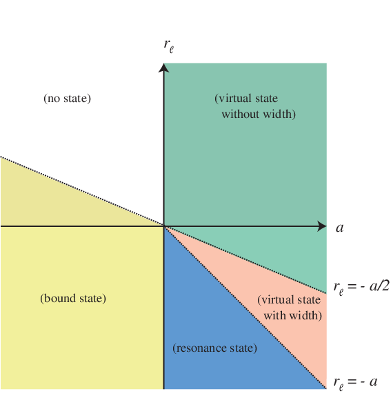
The case corresponds to a bound state or a virtual state without width, while a virtual state with finite width or a resonance can be formed for the case . For later convenience, we schematically illustrate the pole position and the resonance/virtual/bound state in Fig. 2. The poles with () are mapped onto the first (second) Riemann sheet of the energy plane. As mentioned, there are always two poles for given , but the scattering amplitude above the threshold is mainly affected by the pole close to the scattering region (triangles in Fig. 2). In the following, we classify the solutions by the character of the pole most relevant to the amplitude, which appears at larger for the state without the width or at for the state with the width.

Let us first consider the case. The parameter region for is given by
| (35) |
The pole positions are
In this case, both the two solutions lie on the imaginary axis. We can further classify the solutions by the values of and :
| (36) |
Note that means , which corresponds to the case where and has the opposite sign. Thus, in terms of and , we have
| (37) |
Next we consider the case. The parameter region is given by
| (38) |
The real and imaginary parts of the pole can be extracted from Eq. (34) as
In this case, the pair of poles should emerge in the symmetric position with respect to the imaginary axis. If , two poles with finite width appear in the first Riemann sheet of the complex energy plane. Since such poles are forbidden by the causality, we consider them to be an artifact of the truncated effective range expansion and expect them to disappear when higher order terms in are included. We therefore classify the region of giving rise to such poles as “no state”. From Eq. (38), we find that this is the case for . For , the two poles are interpreted as a virtual state with width or a resonance state, depending on the ratio of the real and imaginary parts. The boundary in the complex plane for the virtual and resonance state (with nonrelativistic kinematics ) is given by in the second Riemann sheet, namely
| (39) |
The classification of the solution is then given by
| (40) |
Thus, combining (38) and (40), the parameter space for obtaining resonance/virtual state is given by
| (41) |
We summarize Eq. (37) and (41) in - plot in Fig. 3. If is negative, there is a bound state. For positive , the ratio of and determines the location of the singularities. Setting , we recover the classification by the scattering length Eq. (33).
To illustrate the relation between the threshold parameters and pole position of the amplitude, we solve the single-channel version of the model shown in section 2.2. We choose the channel where we obtain a resonance state with the subtraction constant . The scattering length and effective range are
in accordance with the resonance solution in (41), . When we increase the absolute value of the subtraction constant, the interaction strength is effectively enhanced [2], so the pole is expected to become a virtual state and eventually a bound state.
We calculate the scattering length, the effective range and the pole positions by varying the subtraction constant from to as shown in Fig. 4. The effective range is shown with opposite sign for comparison. As the absolute value of the subtraction constant is increased, both the scattering length and effective range become large. The resonance pole moves to the lower energy region with decreasing the width. This indicates the effective enhancement of the interaction strength.


In contrast to the mild dependence of the effective range, the scattering length increase rapidly for . At , the scattering length becomes larger than the effective range with negative sign. At the same time, the resonance pole moves below the threshold and becomes a virtual state with finite width. When the subtraction constant reaches , the half of the scattering length exceeds the effective range . This coincides with the appearance of the virtual state pole on the real axis. As we further increase the magnitude of the subtraction constant, the pole finally becomes a bound state for . Before that, the scattering length becomes very large positive value. Once the bound state is formed, the scattering length is obtained as a negative value whose absolute value is decreasing. These behaviors are fairly consistent with the classification given in Eqs. (37) and (41).
References
- [1] R. H. Dalitz and S. F. Tuan, Phys. Rev. Lett. 2, 425 (1959); Annals Phys. 10, 307 (1960).
- [2] T. Hyodo, D. Jido and A. Hosaka, Phys. Rev. C 78, 025203 (2008).
- [3] N. Kaiser, P. B. Siegel, and W. Weise, Nucl. Phys. A594, 325 (1995).
- [4] E. Oset and A. Ramos, Nucl. Phys. A635, 99 (1998).
- [5] J. A. Oller and U. G. Meissner, Phys. Lett. B500, 263 (2001).
- [6] M. F. M. Lutz and E. E. Kolomeitsev, Nucl. Phys. A700 (2002) 193.
- [7] E. Oset, A. Ramos and C. Bennhold, Phys. Lett. B527 (2002) 99.
- [8] T. Hyodo, S. I. Nam, D. Jido, and A. Hosaka, Phys. Rev. C 68, 018201 (2003); Prog. Theor. Phys. 112, 73 (2004).
- [9] D. Jido, J. A. Oller, E. Oset, A. Ramos and U. G. Meissner, Nucl. Phys. A 725, 181 (2003).
- [10] B. Borasoy, R. Nissler and W. Weise, Phys. Rev. Lett. 94, 213401 (2005); Eur. Phys. J. A25 (2005) 79.
- [11] B. Borasoy, U.G. Meissner, and R. Nissler, Phys. Rev. C 74, 055201 (2006).
- [12] A. Cieply and J. Smejkal, Eur. Phys. J. A 43, 191 (2010).
- [13] Y. Akaishi and T. Yamazaki, Phys. Rev. C65, 044005 (2002); T. Yamazaki and Y. Akaishi, Phys. Rev. C 76, 045201 (2007).
- [14] K. Nakamura [Particle Data Group], J. Phys. G 37, 075021 (2010).
- [15] T. Hyodo and W. Weise, Phys. Rev. C 77, 035204 (2008).
- [16] P. J. Fink, Jr., G. He, R. H. Landau and J. W. Schnick, Phys. Rev. C 41, 2720 (1990).
- [17] D. Jido, A. Hosaka, J. C. Nacher, E. Oset and A. Ramos, Phys. Rev. C 66, 025203 (2002).
- [18] T. Hyodo, A. Hosaka, M. J. Vicente Vacas and E. Oset, Phys. Lett. B 593, 75 (2004).
- [19] V. K. Magas, E. Oset and A. Ramos, Phys. Rev. Lett. 95, 052301 (2005).
- [20] L. S. Geng, E. Oset and M. Doring, Eur. Phys. J. A32 (2007) 201.
- [21] D. Jido, E. Oset and T. Sekihara, Eur. Phys. J. A42 (2009) 257; See also, ibid. A47 (2011) 42.
- [22] O. Braun et al., Nucl. Phys. B 129, 1 (1977).
- [23] K. Moriya and R. Schumacher [CLAS Collaboration], Nucl. Phys. A 835, 325 (2010).
- [24] J. Siebenson, L. Fabbietti, A. Schmah, E. Epple for the HADES Collaboration, PoS B ORMIO2010, 052 (2010).
- [25] M. Noumi et al., J-PARC proposal E31 “Spectroscopic study of hyperon resonances below threshold via the reaction on Deuteron” (2009).
- [26] Y. Ikeda, H. Kamano and T. Sato, Prog. Theo. Phys. 124 533 (2010).
- [27] Y. Nogami, Phys. Lett. 7, 288 (1963).
- [28] Y. Ikeda and T. Sato, Phys. Rev. C 76, 035203 (2007).
- [29] N. V. Shevchenko, A. Gal, and J. Mares, Phys. Rev. Lett. 98, 082301 (2007); N. V. Shevchenko, A. Gal, J. Mares and J. Revai, Phys. Rev. C 76, 044004 (2007).
- [30] A. Dote, T. Hyodo and W. Weise, Nucl. Phys. A 804, 197 (2008); Phys. Rev. C 79, 014003 (2009).
- [31] S. Wycech and A. M. Green, Phys. Rev. C 79, 014001 (2009).
- [32] Y. Ikeda and T. Sato, Phys. Rev. C 79, 035201 (2009).
- [33] D. Jido, T. Sekihara, Y. Ikeda, T. Hyodo, Y. Kanada-En’yo and E. Oset, Nucl. Phys. A 835 (2010) 59.
- [34] A. D. Martin, Nucl. Phys. B179, 33 (1981).
- [35] U. G. Meissner, U. Raha and A. Rusetsky, Eur. Phys. J. C 35, 349 (2004).
- [36] D. N. Tovee et al., Nucl. Phys. B 33, 493 (1971).
- [37] R. J. Nowak et al., Nucl. Phys. B 139, 61 (1978).
- [38] J. Esmaili, Y. Akaishi and T. Yamazaki, Phys. Lett. B686 23 (2010).
- [39] T. Hyodo, D. Jido and A. Hosaka, Phys. Rev. Lett. 97, 192002 (2006); Phys. Rev. D 75, 034002 (2007).
- [40] T. Hyodo and M. Oka, in preparation.
- [41] N. Cabibbo, Phys. Rev. Lett. 93, 121801 (2004).
- [42] Y. Ikeda, et al., HAL QCD collaboration, in preparation.